Article

Geo-Spatial Mapping of Hate Speech Prediction in Roman Urdu

by
Samia Aziz
1,
Muhammad Shahzad Sarfraz
1,
Muhammad Usman
1,
Muhammad Umar Aftab
1 and
Hafiz Tayyab Rauf
2,*
1
Department of Computer Science, National University of Computer and Emerging Sciences, Islamabad, Chiniot-Faisalabad Campus, Chiniot 35400, Pakistan
2
Centre for Smart Systems, AI and Cybersecurity, Staffordshire University, Stoke-on-Trent ST4 2DE, UK
*
Author to whom correspondence should be addressed.
Mathematics 2023, 11(4), 969; https://doi.org/10.3390/math11040969
Submission received: 9 December 2022 / Revised: 8 February 2023 / Accepted: 11 February 2023 / Published: 14 February 2023
(This article belongs to the Special Issue New Insights in Machine Learning and Deep Neural Networks)

Abstract

:
Social media has transformed into a crucial channel for political expression. Twitter, especially, is a vital platform used to exchange political hate in Pakistan. Political hate speech affects the public image of politicians, targets their supporters, and hurts public sentiments. Hate speech is a controversial public speech that promotes violence toward a person or group based on specific characteristics. Although studies have been conducted to identify hate speech in European languages, Roman languages have yet to receive much attention. In this research work, we present the automatic detection of political hate speech in Roman Urdu. An exclusive political hate speech labeled dataset (RU-PHS) containing 5002 instances and city-level information has been developed. To overcome the vast lexical structure of Roman Urdu, we propose an algorithm for the lexical unification of Roman Urdu. Three vectorization techniques are developed: TF-IDF, word2vec, and fastText. A comparative analysis of the accuracy and time complexity of conventional machine learning models and fine-tuned neural networks using dense word representations is presented for classifying and predicting political hate speech. The results show that a random forest and the proposed feed-forward neural network achieve an accuracy of 93% using fastText word embedding to distinguish between neutral and politically offensive speech. The statistical information helps identify trends and patterns, and the hotspot and cluster analysis assist in pinpointing Punjab as a highly susceptible area in Pakistan in terms of political hate tweet generation.

1. Introduction

The recent couple of years have seen drastic growth in social networks and the rate of content consumers. Social media platforms are used to share posts (Facebook) and tweets (Twitter) that can contain text, images, videos, emotions, etc., directly affecting the daily life of consumers. A significant and slippery type of such language is hateful speech: content that communicates a class’s sentiment. Offensive speech has become a significant issue for everyone on the Web, where consumer-created content appears from the remark areas of information sites to ongoing talk meetings in vivid games. Such content can embarrass consumers and can furthermore support radicalization and incite violence [1]. Twitter is among the leading social media platforms. A 140-character post is called a tweet and can include spaces, emojis, URLs, and hashtags. According to the latest survey [2], 217 million active monetizable users and 500 million tweets are produced daily. Twitter restricts consumers from posting hateful and contemptuous substances [3].
The Urdu language has over 230 million speakers worldwide, including in the UAE, the UK, and the US. The overall active social media stats of Pakistani users are depicted in Figure 1. Urdu is the official language of Pakistan, a rank it imparts to English in a nation of 226 million people. Despite that, there are a few difficulties related to Urdu writing. The Urdu language comprises 40 letters. The standard consoles are intended to only deal with the 26 letters of English. This enormous gap between various alphabets makes it almost difficult to write Urdu letters using a standard English console. Urdu is a morphologically rich language that bears a shortfall of resources. It has a complex inflectional framework, a course of word improvement wherein things are added to the root word to demonstrate syntactic implications. Roman Urdu (RU) is the conventional name utilized for the Urdu language written in Roman script.
Provided the volume of information growth of social media platforms, especially on Twitter, where users express their opinions, feelings, and surprising/devastating news in RU, they may also leave inappropriate content such as hate speech. The main parts of the problem statement in this research are that online hate speech can set off extreme occasions in society [4]. Current methods, such as word embeddings, are only available for English or asset-rich languages [5]. Present hate speech detection procedures do not perform unequivocally on the code-mixed imperfect, informal, and resource-poor languages [6].
The principal objective was classifying hate speech to identify and analyze data from social networks, especially Twitter, using standard machine learning methods for text classification and evaluation. The content on social media posted each minute is usually unrefined and represents one’s beliefs; people express and judge others based on their choices, ultimately creating circumstances for others and even societies. For example, discussion on religion and politics almost always results in violence. For this research, the aim was to target offensive political speech written in RU script. The tweets were targeted based on infamous political keywords that could potentially contain RU data and offensive speech. The offensive speech data were obtained from Twitter. Several objectives designed for this research could help classify, predict, and geomap offensive speech written in RU. The main contributions of this research are as follows:
  • This research work contributes to a detailed analysis of current approaches employed for the classification of hate speech in Roman Urdu. It also presents a review of the literature on data sets developed by previous studies and a comparative analysis that highlights the strengths and weaknesses of these studies.
  • This research proposes a complete dataset of Roman Urdu political hate speech (RU-PHS) containing 5002 instances along with their labels and city-level location information.
  • To overcome the vast lexical structure of Roman Urdu, an algorithm for the lexical unification of Roman Urdu is proposed, by leveraging regular expressions.
  • A comparative analysis between conventional machine learning models, a feed-forward neural network, and a conventional neural network using dense word representations (i.e., TF-IDF, word2vec, and fastText) is presented for the classification and prediction of political hate speech.
  • A spatial data analysis of the RU-PHS dataset in terms of hotspots and clusters is conducted to predict future affected areas in Pakistan.
The paper is organized as follows: In Section 2, we discuss preliminary concepts of text classification, its applications, and state-of-the-art approaches with contemporary trends and open problems. This is followed by Section 3, in which a comprehensive review of the literature related to the scope of this research study is presented. Section 4 presents the proposed methodology for the said problems. Section 5 discusses the implementation, dataset description, and formulation process. Section 6 presents the spatial analysis and results of data points. Section 7 addresses the hyperparameter settings for the proposed models and evaluates their performance. Lastly, Section 8 presents the conclusions and future directions.

2. Preliminaries

2.1. Text Classification

Text or document classification organizes, structures, and sorts text into binary or multiple classes. Over the past several decades, text classification problems have been widely studied and addressed in a variety of real-life domains [7]. Researchers are now interested in developing applications that use text classifiers, especially given the recent advancements in natural language processing (NLP) and data mining.
Classifying text into different categories starts using plain raw text files stored on the disk. It then involves data cleaning, preprocessing, and transformation. The transformed data are then preprocessed for the machine learning algorithm; this step is known as feature engineering and converts words into features for training classification and predictive models. Figure 2 gives a classic representation of the training of a machine learning classifier to classify text. Labels are provided along with the text data to train a machine learning algorithm. The data preprocessing steps are performed, including tokenization, lower casing, stop word removal, stemming, and lemmatization.
The feature engineering steps convert words into meaningful information such as frequencies using TF-IDF and one-hot encoding; for a dense representation, word2vec, fastText, and Glove word embeddings are used to capture contextual information. Once the features are extracted, they are passed to the ML models, which then learn to classify the data into given categories. Figure 3 represents the prediction process, where the ML model is not provided with labels to test what the model has learned from the training data.

2.2. Sentiment Analysis

Sentiment analysis is the process of determining if a user-generated post is positive, negative, or objective. NLP is used in an emotion detection analysis system. Machine learning algorithms assign weighted sentiment values to entities, topics, documents, and categorizations within a statement or phrase. It helps corporations get an idea of how well or poorly their product or service is performing on the market by analyzing the general sentiment of reviews and conversations on social networks. Opinion research is also used to distinguish positive or hostile public sentiments communicated on sites about culture, race, or orientation that could cause viciousness and hostility between individuals of various backgrounds. The sentiment investigation task centers around distinguishing and extracting feelings from a message to a specific subject or item. A subtask of sentiment examination is the opinion order in light of specific polarities [8].

2.2.1. Fine-Grained

The fine-grained sentiment analysis model analyzes the sentence by dividing it into clauses or phrases. It helps to gain polarity precision. A phrase is divided into expressions or clauses, and every fragment is examined in association with others. We can recognize who discusses an item and what an individual discusses in their criticism. We can regulate a sentiment analysis across the subsequent polarity classes: neutral, positive, negative, and offensive. The fine-grained analysis is beneficent when analyzing reviews or ratings.

2.2.2. Aspect Based

The aspect-based sentiment analysis focuses on the features mentioned in a phrase that is later classified as an emotion. This model dives deeper and helps detect the specific aspects that people talk about in their posts.

2.2.3. Emotion Detection

The emotion detection sentiment analysis model goes way beyond just polarity count. It helps recognize emotions embedded in phrases such as happiness, sadness, frustration, anger, fear, panic, etc. This model utilizes lexicon-based approaches to analyze the word level that delivers a specific emotion. Some state-of-the-art classifiers also use strong artificial intelligence techniques. It is prescribed to involve machine learning over lexicons since individuals express feelings in many ways. For instance, the line “This movie is going to kill me” might communicate sensations of dread and frenzy.

2.2.4. Intent Analysis

As the name suggests, intent sentiment analysis helps detect a consumer’s intentions. Based on consumers’ shopping behaviors, are they interested in buying or are they just browsing? Precisely recognizing users’ intent helps save organizations time and money. Thus, often, organizations pursue purchasers that want to avoid purchasing in the short term. An exact intent investigation can determine this obstacle. In this way, if a consumer has a history of buying things online, a corporation can target them with marketing. If they never buy online, time and assets can be saved by not advertising to those consumers.

3. Related Work

In this digital age, since web-based hate speech content began to become viral on various social media stages, additional research has been conducted on detecting, classifying, and predicting hostile speech. Nevertheless, only some text corpora have been produced in RU containing a minimal dataset. A prior work [4] introduced RU toxic comment identification. They presented an extensive corpus containing 72,000 labeled comments with a substantial interannotator agreement. They worked with existing machine learning methods that performed well for English language toxic datasets incorporating text classification techniques and recent deep-learning-based models. This study’s principal challenge was the inaccessibility of pretrained word embeddings in RU, so they created different word embeddings utilizing Glove, word2vec, and fastText procedures. They achieved the highest scores in word embeddings utilizing the skip-gram model of fastText.
In [5], research work by Rizwan Ali Naqv et al. aimed to develop a Roman Urdu news classifier. For this, they scraped data from news websites and divided it into five classes: international news, health, sports, business, and technology. They collected a total of 735 news texts that belonged to the categories mentioned. This data set was collected in Urdu and later translated into RU using ijunoon.com. They faced the challenge of lexical variations of RU in this study. To handle this problem, they divided their test data set into two parts with lexical variations (real-world test data) and without lexical variations. To extract features from this news dataset, the study used (TF-IDF).
In addition to unsupervised machine learning techniques, studies such as that by Nobata et al. [9] introduced the utilization of supervised ML techniques for recognizing offensive speech. Of these research studies, the first research study gathered publicly available commentary from the financial and news domains and generated a body of offensive speech. Furthermore, research was carried out involving syntactic features and various kinds of embedding techniques. Moin Khan et al. [10] developed an RU corpus composed of over 5000 tweets, most of which were hate speech. They divided the tweets into hostile and neutral at first and further sorted the hostile tweets into offensive and hate speech. They involved a few supervised learning technique strategies for assessing the developed corpus. Logistic regression performed best in their study to distinguish between neutral and hostile sentences. Hammad Rizwan et al. [11] proposed a dataset named RUHSOLD with 10,012 tweets in RU and labeled them into five hate speech classes, including abusive, profane, sexism, religious hate, and normal. A novel approach, CNN-gram for offensive speech classification, was proposed and a comparative analysis of their proposed model was performed with various baseline models using the RUHSOLD dataset.
The study [12] examined several methods for classifying offensive speech on social media platforms. They introduced an integration of lexicon-based and machine-learning-based techniques for hate speech prediction. They notably used emotional information in a sentence to help get a better accuracy in offensive speech detection. They performed a statistical analysis to determine the critical correlation between the probability that the consumer would share comments related to the base class, and the tagged labels related to that class. The review achieved correlation coefficient values for racism and sexism of 0.71 and 0.76, respectively. Additional research by Muhammad Bilal et al. [13] on RU opinion mining evaluated three classification algorithms: naive Bayes, decision tree, and KNN. They extracted opinions from an online blog and labeled them positive and negative. These labeled data were further supplied to the models, and naive Bayes outperformed all the others in terms of accuracy, recall, precision, and F measures.
Various studies have generated Roman Urdu hate speech corpora and made them publicly available. Table 1 summarizes the Roman Urdu datasets generated along with their name, size, and language. A novel study [14] conducted research on generating a parallel corpus for Urdu and RU. They presented a large-scale RU parallel corpus named Roman-Urdu-Parl that contained 6.37 million Urdu and RU text pairs. These data were collected from various sources. The crowd-sourcing technique was used to annotate the data set. It contained a total of 42.9K unique words for RU and 43.8K unique words for Urdu. This study mainly focused on word representation learning and its machine transliteration and vector representation. Despite the traditional techniques to perform sentiment analysis, such as lexical normalization, word dictionary, and code transfer indication, a study [15], independent of these techniques, proposed a sentiment analysis using multilingual BERT (mBERT) and XLM-RoBERTa (XLM-R) models. They acquired the Twitter data set during the 2018 election named MultiSenti. It contained code-mixed English and RU. The dataset, after preprocessing, was divided into three classes that include positive, negative, and neutral. XLM-Roberta gave higher accuracy and F1 score for informal and under-resource languages such as code-mixed English and RU.
Roman Urdu datasets were acquired using different platforms. Table 2 gives a summary of the famous platforms used for this matter, in which Twitter has been used most frequently in research studies.
Mukand [17] introduced a technique for extremity characterization of code-mixed data. The technique was based on a hypothesis, namely SCL (structural correspondence learning), used in domain adaptation. The transliteration oracle handled the problem with spelling variations. A transliteration oracle is a transliterate processor that converts strings based on the sound they represent from one writing system (such as Latin) to another (such as Arabic). The authors of the paper used two types of translation oracles—the first oracle, which accommodated spelling variations, and the second oracle, which was a translation between Urdu and English. Using a double metaphone algorithm, the first oracle completely switched all tokens to RU. Tokens that had the same metaphone code in both target and source languages were added into pivot pairs. The second oracle accomplished the interpretation between Urdu and English.
Research carried out by Kaur et al. [54] in 2014 proposed a hybrid approach for Punjabi text classification. This exploration utilized a number of naive Bayesian and N-gram methods. The elements of the N-gram method were extracted and then used as a training data set to train a naive Bayes classifier. The algorithm was then tested by providing testing data. The observation was made that the results from previously proposed frameworks and the current algorithm gave a promising number of clarifications. Studies have employed different techniques to solve these problems, and an analysis of the strengths and weaknesses of these studies are presented in Table 3. Another approach was used by Ashari et al. in [55] in which they classified using naive Bayes, decision tree, and KNN classifiers and proposed three classification models to design an alternative solution using WEKA as an information mining instrument. Their investigations showed that decision tree was the quickest and KNN computations took time, so it was a slow characterization strategy. The explanation they referenced was that, in the decision tree, there was no computation included. Characterization by adhering to the tree guidelines was faster than those that required computation in the NB and KNN classifiers.
In 2012, another study on sentiment analysis was carried out by Jebaseeli [65] in which they explored the use of three classifiers, namely, NB, KNN and RF, for the classification of sentiments as positive or negative about the machine learning structure for inspiration to dissect the ability of these three classifiers. In the study, a data set of 300 surveys was taken with a split of 100 positive, 100 negative, and 100 neutral surveys [65]. In the preprocessing step, customarily assembling words and just generally utilized words were taken out by utilizing the SVD approach. SVD was utilized to rate the significance of words. The resulting preprocessed information was utilized as responsibility estimation. In that examination, a degree of 55–60% accuracy was achieved. Gamallo [66] presented a set of NB classifiers to determine the polarization of English Twitter posts. Two naive classifiers were compiled: the baseline (designed to portray tweets as specific, negative, and neutral) and the binary classifier. The classifiers took into account phrases (nouns, verbs, adjectives, and adverbs), multiword, and polarities vocabulary from numerous roots. A related study [67] used a psychrometric deep learning model to classify the sentiments of tourists against the COVID-19 pandemic. The comments were collected from Twitter containing information about weather, health, holidays, seasonality, and economics. The proposed model used the PANAS (Positive and Negative Affect Scale) to classify these comments.

4. Proposed Methodology

4.1. Representing Words

The text data presented as input to any machine learning model and coming as output from it are converted to embeddings. These input and output embeddings of words are the parameters of the model, stored in lookup matrices W i and W o . Word embedding methods are employed to demonstrate words and connect humans mathematically—an artificial knowledge of learning.
Word embeddings learn text representations in an n-dimensional space, in which words can be represented in terms of frequency counts, i.e., TF-IDF or words with similar meanings have similar representations. Two similar words are represented by almost identical vectors very close together in a feature space, i.e., word2vec and fastText. These techniques are preferred depending on the data’s status, size, and output preferences. Much work has recently been done with models representing words as functions of subword units. Table 4 shows the words and their decomposition patterns. In this work, we considered two word representations: words and decomposing them into N-grams of characters. This is required for most natural language processing problems. In this section, we present the three types of word representations developed to convert the exclusively collected dataset into vector representations.

4.1.1. TF-IDF

TF-IDF [68] is a quantitative tool that evaluates the relevance of a word in a collection of documents. This is accomplished by simply multiplying metrics: the number of times a word appears in a document and the word’s inverse document frequency along a collection of documents. The higher the score, the more important that word is in that document. To put it mathematically, the TF-IDF score for the word w in document d of document set D is shown in Equation (1). Then, Equations (2) and (3) further drive the term frequency and document frequency.
t f i d f ( w , d , D ) = t f ( w , d ) · idf ( w , D )
where:
t f ( w , d ) = log ( 1 + freq ( w , d ) )
i d f ( w , D ) = log N count ( d D : w d )

4.1.2. word2vec

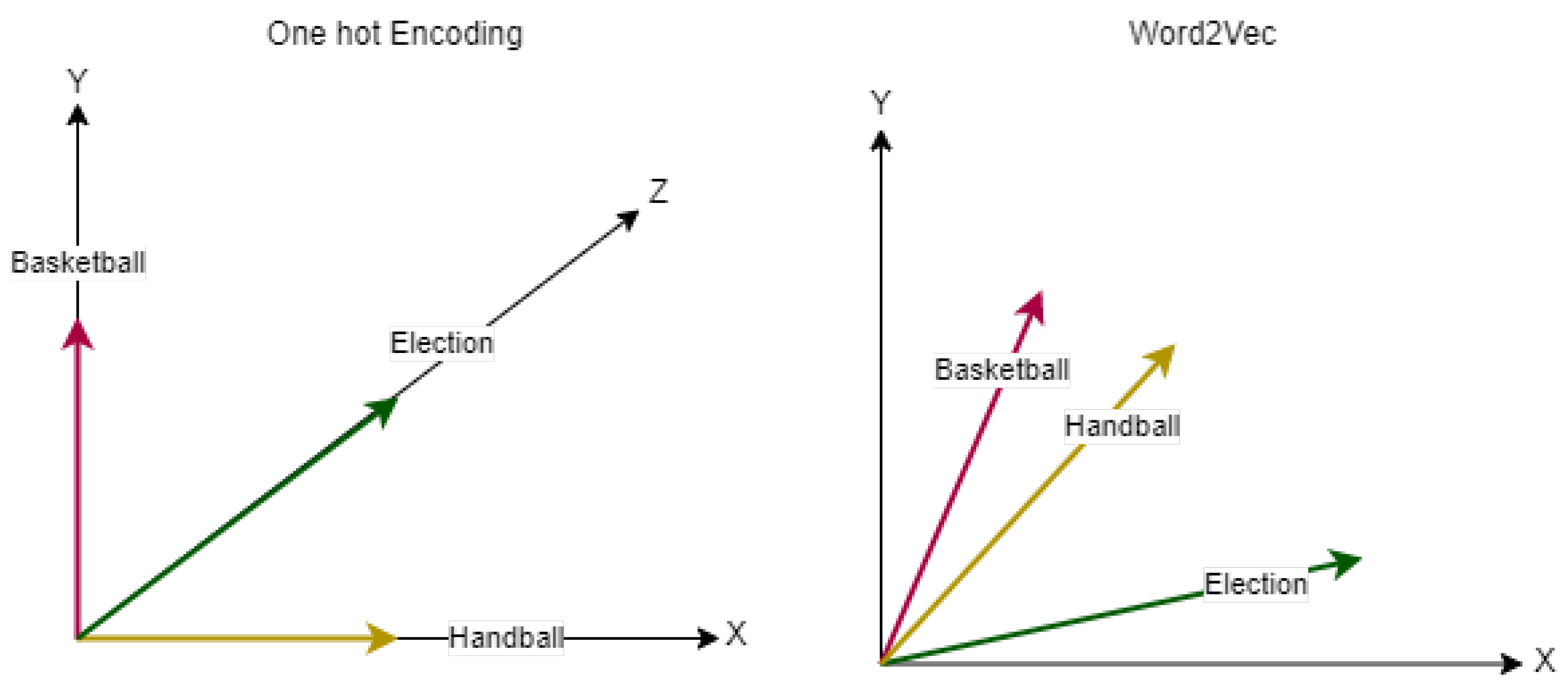
word2vec [69] is a predictive neural word embedding model that uses a neural network model to learn vector representations from a large corpus of text. It predicts the target word by computing the cosine similarity between vectors, i.e., by analyzing nearby words. The following Figure 4 represents how word vectors with similar meanings are clustered in close proximity in word2vec and how a one-hot encoding does not capture context at all.
similarity ( B a s k e t b a l l , H a n d b a l l ) = cos ( θ ) = B a s k e t b a l l · H a n d b a l l B a s k e t b a l l H a n d b a l l
word2vec captures the similarity score between words using the cosine similarity equation when trained on a large corpus. In Figure 4, the vectors X, Y, and Z can be considered dimensions. Each word occupies a dimension for the one-hot encoding and has nothing to do with the rest of the words. Hence, all the words are independent of each other. In word2vec, the main goal is to have words occupy close spatial positions if they are contextually the same. Equation (4) calculates the similarity between such vectors, which is close to one, i.e., the cosine angle is close to zero. This is achieved by taking the product of both vectors, in this case, Basketball and Handball, and dividing it by the product of the lengths of both vectors.
There are two main architectures of word2vec that are used to learn distributed representations.
  • Continuous bag-of-words (CBOW);
  • Continuous skip-gram (CSG).
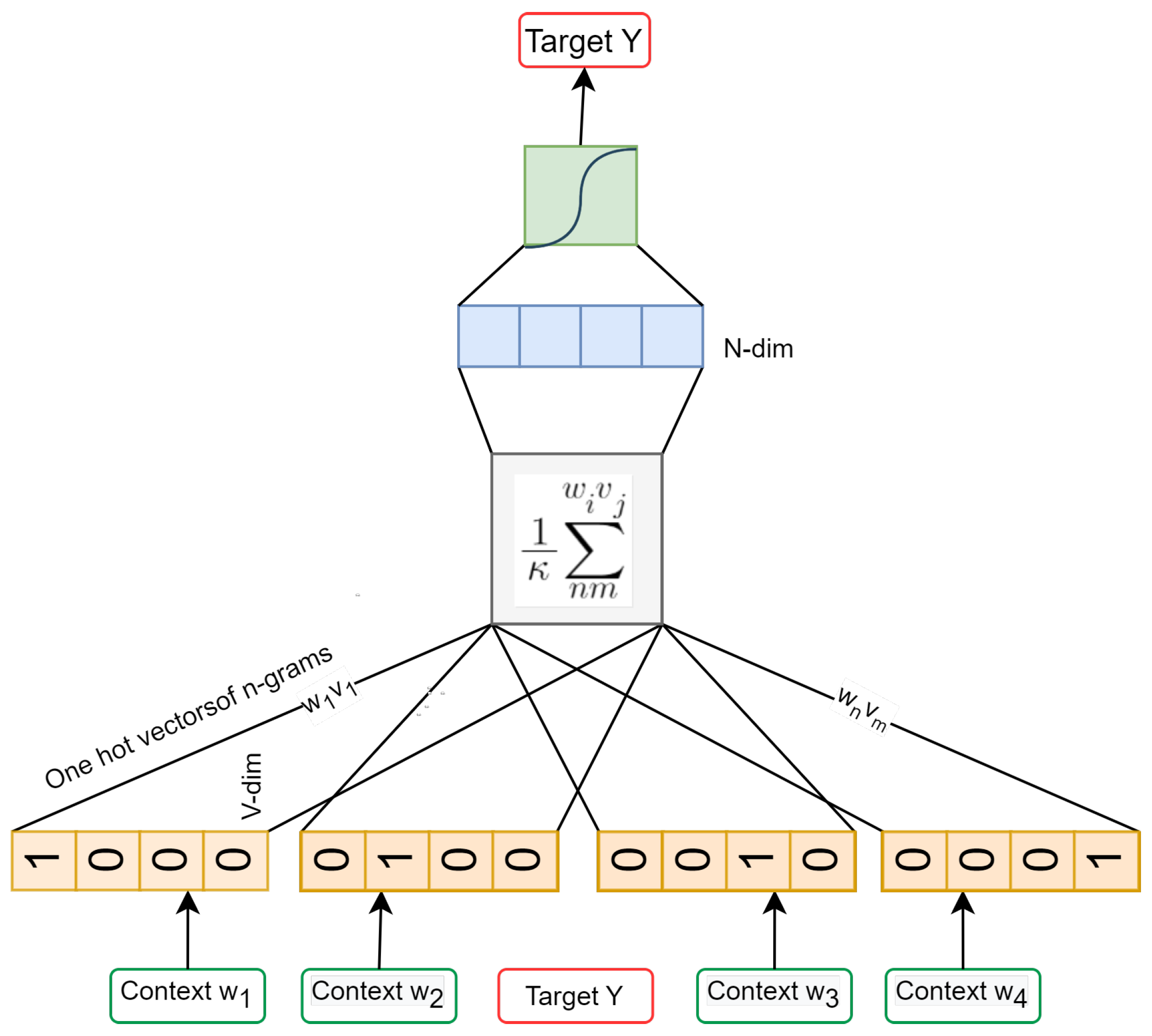
CBOW attempts to predict a word based on a window of surrounding context words, but the bag-of-word assumption is not affected by the sequence of context words, whereas continuous skip gram does the opposite. Based on the input word, the continuous skip-gram model predicts whether words that are surrounding a word also called context words. This model contains one hidden layer, which performs a dot product of the input vector and weight matrix and no activation function is used (see Figure 5). The output vector generated by the hidden layer and the weight matrix of the hidden layer is multiplied together with a softmax function to predict the probability of context words.

4.1.3. fastText

fastText [70] embeddings use subword-level knowledge to generate word vectors. Words are expressed as the sum of gram vectors after learning N-gram representations. This adds information at the subword level to the word2vec framework. This enables embeddings for understanding prefixes and suffixes. Similarly to word2vec, fastText learns the word vectors along with the N-grams that exist within each word, although these embeddings are computationally more expensive than word2vec.

4.2. Machine Learning for Political Hate Speech Detection

4.2.1. Feed-Forward Neural Network

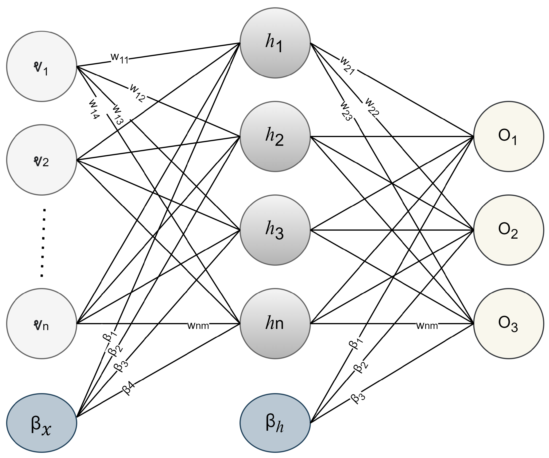
A feed-forward neural network is the oldest and most fundamental type of artificial NN in which node links do not constitute a loop [71]. Feed-forward neural networks are made of an input layer, n numbers of hidden layers, and an output layer where the neurons of the input and hidden layers carry weights and the data only move in one direction, i.e., in a forward fashion (see Figure 6). In this case, the input or embedding layer takes the distributed representations V of words W generated by the word2vec and fastText models.
L R d r × | V |
It takes the vocabulary size and maximum input length of words in the vocabulary as embedding layer features. Vectors are denoted as r R d r and are represented in practice by a lookup matrix L; see Equation (5). In this lookup matrix L, every row has a continuing vector that belongs to words existing in the vocabulary and is called the word embedding, represented as shown in Equation (6).
L = r j j = 1 | V |
After the input layer, where the data are fed to input neurons in the shape of feature vectors, the values and their assigned weights are then fed-forward to the hidden layers, where the magic happens. Each hidden layer transforms the values linearly with a weight metric W (shown in Equation (7)) and β as a bias vector β h R d h .
W i , j h R d n × ( n 1 ) d r
This is then followed by applying an activation function (shown in Equation (8)) to induce nonlinearity into the network. It helps simulate whether the neuron fires or not, prevents overfitting, and speeds up the convergence. In Equation (8), W i , j h represents the product of the input vectors and the weights of the hidden layer, and b h represent the bias of the hidden layers h t . Finally, in the output layer, these hidden representations are mapped to a probability distribution. This implies that we must assign a probability to every word in the dictionary.
h t = ϕ W i , j h v i + b h

4.2.2. Convolutional Neural Network

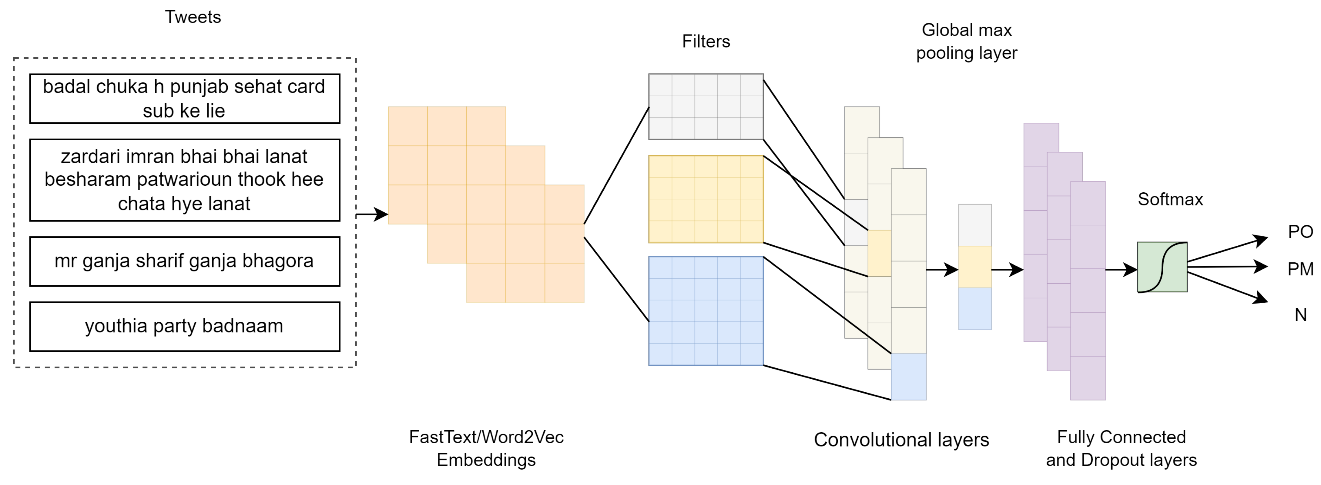
Convolutional neural networks (CNNs) [72] were initially developed to recognize digits, especially handwritten ones from images. The main functionalities of a CNN are convolutional and pooling layers to retrieve features from the input data. For Roman Urdu hate speech classification, we fine-tuned a 1D CNN model. The block diagram of the proposed architecture can be seen in Figure 7.
A convolution layer is a sliding window that converts feature vectors from a fixed-size region. Pooling layers are typically used after a convolutional layer to reduce dimensionality and provide a fixed-length output. For example, max pooling takes the maximum value from the previous convolutional layer. The pooling output is usually passed to a fully connected layer, which is functionally equivalent to a typical multilayer perceptron neural network (MLP). For text classification tasks, a 1D array represents the text, and the architecture of the CNN becomes 1D convolutional and grouping operations. The CNN model used for classifying labeled Roman Urdu tweets contained five layers: the input layer as an embedding layer, a 1D convolutional layer, one global max pooling layer, and two dense layers. The input size had dimension 200, and the output had dimension 3. The CNN computed the operations’ results and the loss function gradient using forward and backward propagation.
z i = ω 1 , ω 2 , ω i + k R k × D
Given a sequence of n words w 1 , w 2 , w n , where each word belongs to the word vocabulary W c and embedding vector with dimension D c , the word embedding matrix is C = R D c × W c . The sentences are passed to this embedding matrix and converted to vectors. The 1D convolution is produced by sliding a window of size k with the same convolutional filters and kernels in every sliding window throughout the sequence. With a dot product between the embedding vectors v and the weight w and the convolution of width k, the concatenated embedding vector of the ith sliding window is shown in Equation (9).
Since in forward propagation, the input data are fed to the neural network in the forward direction to calculate output vectors from input vectors at each layer l, the forward propagation in a one-dimensional convolutional network is shown in Equation (10).
s n l = β n l + i = 1 N l 1 conv ω i = 1 l 1 , o i l 1
where β n l is the bias of the nth neuron at layer l, and o i l 1 expresses the output of the ith neuron at layer l 1 . For each sliding window i, the scaler values s i are generated by applying convolutional filters to each of them, that is, s i = g z i . v R . Features extracted from this layer are then passed to a 1D convolutional layer which in the implementation had a filter size of 5, i.e., u 1 , u 5 multiplied by a matrix U and adding bias β l at layer l. Each layer receives the input and calculates the output with an activation function which was a ReLu in this implementation (shown in Equation (11)).
s i = g z i . U + β
This output is then forwarded to the next layer in the network, along with the learning rate η , the weights of the kernel are updated using the following Equation (12).
ω i k l 1 ( p + 1 ) = w i k l 1 ( p ) η E w i k I 1 ( p )
Since the values assigned to the biases are learnable, just like the weights, the biases are also updated (shown in Equation (13)). p and p + 1 represents the current state and next state. E represents the mean square error (MSE) between observed values and actual values at a given layer.
β k l ( p + 1 ) = β k l ( p ) η E β k l ( p )
This is followed by a pooling layer, i.e., a global max pooling. It combines all the resultant vectors produced by the convolutional layer into a one-dimensional feature vector. Max pooling is done by taking the max value from the resultant vector as shown graphically in Figure 7. This 1D vector captures the most important features from the sentence and maps them to classification labels. Furthermore, dropout layers are added, randomly dropping half of the neurons, a common method for reducing overfitting in neural networks, before passing through to the output layer, where a prediction is made.

5. Implementation

5.1. RU-PHS Dataset

To validate the effectiveness of our proposed methodology, a benchmark dataset was developed named Roman Urdu Political Hate Speech. This entire dataset contained a total of 5001 labeled Roman Urdu tweets. Each row contained text with its corresponding labels and their respective city-level locations. It did not contain any null values. The data set was categorized into three classes, PO, PM, and N, described in Table 5. Of the 5K tweets, 3028 were labeled as politically offensive, 1190 as politically medium, and 784 as neutral.

5.2. Preprocessing

Text data are typically unstructured, especially data scraped from social networks, as it is user-generated content. While Roman Urdu writing lacks rules and has no standard lexicon, users write a given word with their own set of rules with several spelling variations. This creates the need to normalize the data and transform it into a structured feature space. The data set was collected from the social media platform Twitter for this research work. The data set was based on trending political hate words from January 2022 to April 2022. Data were collected using an R script, and Twitter Python API was used to stream the data set, which allowed the use of the Twitter developer portal for us to retrieve tweet data.
The scraped data contained more than 30 columns of information for each tweet irrelevant to this investigation. Only the columns “Text” and “Location” were obtained from it. These data were further filtered based on the location, and only tweets from Pakistan were retained. Data were preprocessed using regular expressions (re) to remove @mentions, #Hashtags, URLs, Unicode characters, emojis, and white spaces and converted to lowercase. Furthermore, the dataset was imbalanced since the “politically medium” and “neutral” classes had comparatively fewer samples. To generate synthetic samples for the minority class, the SMOTE algorithm was used. SMOTE is an oversampling technique, which helps produce new samples by focusing on the feature set and interpolating between positive samples that lie together. The total sample distribution of the dataset was (5002, 3), and after SMOTE balancing, the total samples of all three classes were transformed to (9084, 3); only the minority classes were oversampled based on the max number of samples of the majority class, which was 3028.

5.2.1. Guideline Development

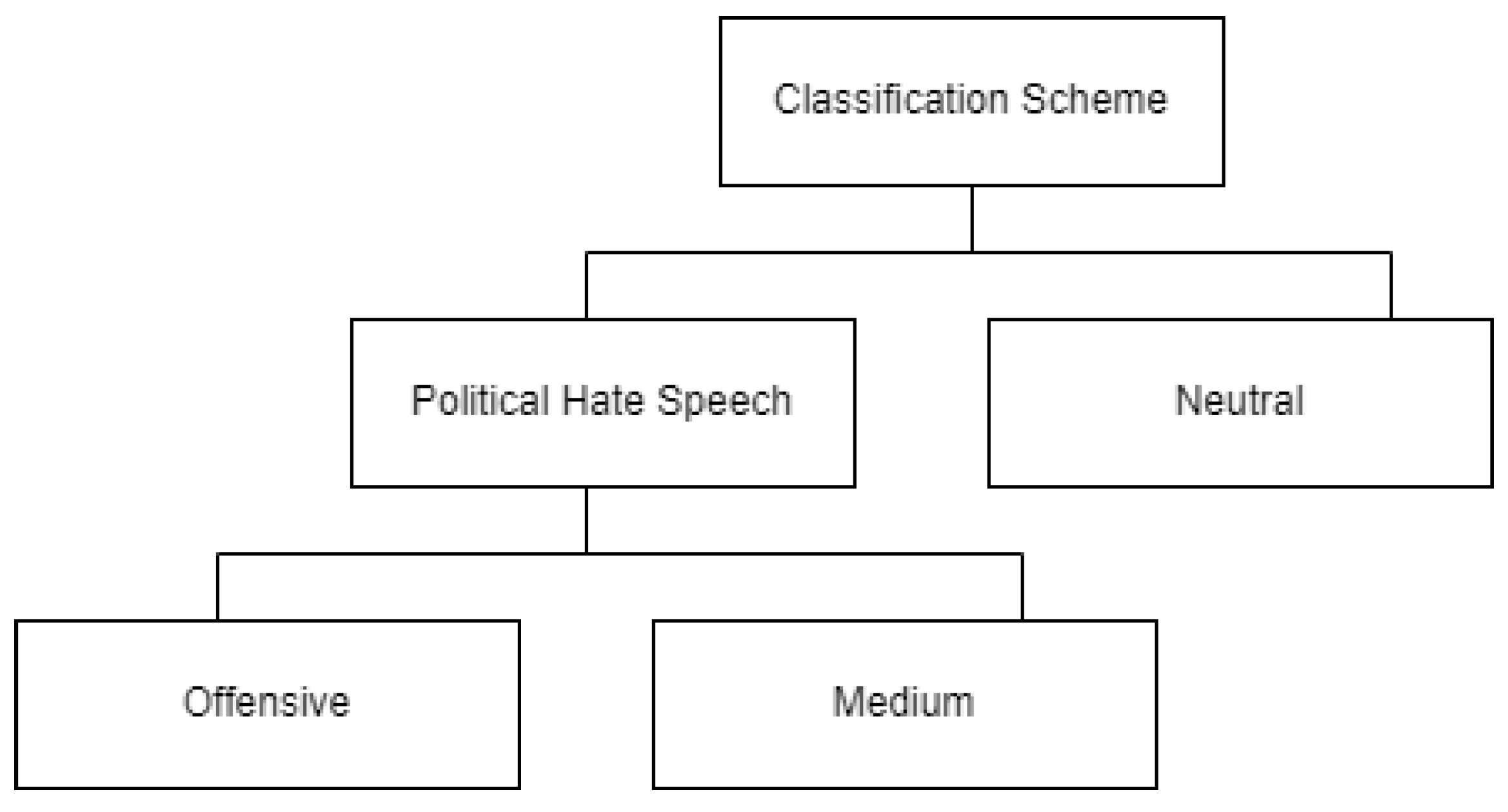
For the development of guidelines, we designed a constant procedure to form a strictly exhaustive set of guidelines to determine whether a given phrase or tweet was hate speech. The essential advantage of this guideline development was the consistent approach that would form with their use and lead to correct annotations. The following Table 6 highlights the first-level classification guidelines for offensive speech identification. There were two levels of classifications. The first level classified hate speech and neutral expressions. In the second-level classification for this research, we aimed to classify political hate speech into further three categories: neutral, medium, and offensive. An overall review of the scraped tweets after cleaning was conducted. It was revealed that there was a sizable number of unwanted tweets that were neither neutral nor offensive and did not lie under political hate speech. Since our primary focus was non-English data for this research, all the tweets were split into English and non-English content. A semiautomated technique of NLTK’s language detection feature was developed to identify candidate corpus for further manual labeling of the data.

5.2.2. Data Annotation

In this step, machine classifiers were used to learn the characteristics of Twitter posts that represented the class to which they belonged to complete this subjective task using a large-scope data analysis critical for the volumes of data created. In the next step, we manually identified and annotated tweets using the guidelines developed, as machine learning classifiers needed to be fed more information to classify the data correctly. RU data needed predefined rules and regulations to write its roman counterpart, making it difficult to label the data automatically. Thus, the collected data were partly annotated using machine learning algorithms and partly annotated by a human annotator. The annotator was a native speaker of the Urdu language and a graduate. Figure 8 represents the taxonomy developed for the classification of hate speech.

5.2.3. Custom Stop Words

Stop words are known as conjunction terms or “Haroof e Jaar” in Urdu. A similar list of stop words is also present for Roman Urdu. The complete removal of stop words has the primary benefit of returning only relevant documents. We removed English stop words from our dataset using NLTK library’s default list of 40 stop words. A predefined list of RU stop words was obtained from GitHub containing 100 words [18]. A custom list of stop words was extracted from the data set (RU-PHS). For this, we counted the frequency of the most commonly occurring words and sorted them in A–Z order using a Python script. For the next step, the standard stop words list was compared to the frequently occurring words list, and the stop word variants contained in the RU-PHS dataset were identified and removed.

5.2.4. Lexical Unification

Roman Urdu lacks standardization rules, especially user-generated data, which are always unstructured, e.g., inconsistent forms of writing words. Since the machine cannot comprehend that one word can be written with many variations, it takes each variation as a whole different word. This can also lead to biased and compromised results in the classification task. To overcome this problem and to map different variations of one word to a single string we proposed to remove vowels from words. The algorithm (shown in Algorithm 1) was designed to find instances of strings that occurred most frequently in the RU-PHS dataset and to remove vowels from those strings. Table 7 represents the transformation of word variations to a normalized form by pruning vowels.
Algorithm 1: RU Lexical Unification by Removing Vowels.
1. Read CSV file containing scraped data
2. Clean the data by removing
 a. @mentions, #hashtags, URLs, and Unicode characters.
 b. White spaces including from the start and end of the line.
 c. Non-English, numeric values, and special symbols.
3. Compute a list F of the most frequently occurring words
   i = 1 n ( string S )
4. Select strings with the highest frequency
max i = 1 n ( string S )
5. Create a list of vowels V
6. Compare each string to the list of vowels
 a. Convert strings to lowercase
 b. For each x in input string S
 c. If x is in V
    Replace it with empty space
   else
    Retain it as it is
7. Replace all instances of the original string in the CSV file with the resultant string.

6. Spatial Data Analysis of Political Hate Speech

Spatial analysis is the process of modeling problems geographically, deriving results through information processing, and then exploring and examining those results. This kind of analysis has proven to be highly effective for assessing the geographic viability of specific locations for various applications, estimating and forecasting outcomes, interpreting and comprehending change, identifying meaningful patterns hidden in data, and much more. In this research, the exclusive political hate speech dataset (RU-PHS) was collected along with locations. The data set was collected only from Pakistan and contained city-level information on each tweet. The aim was to apply geospatial techniques on the dataset to predict hate speech.

6.1. Geocoding

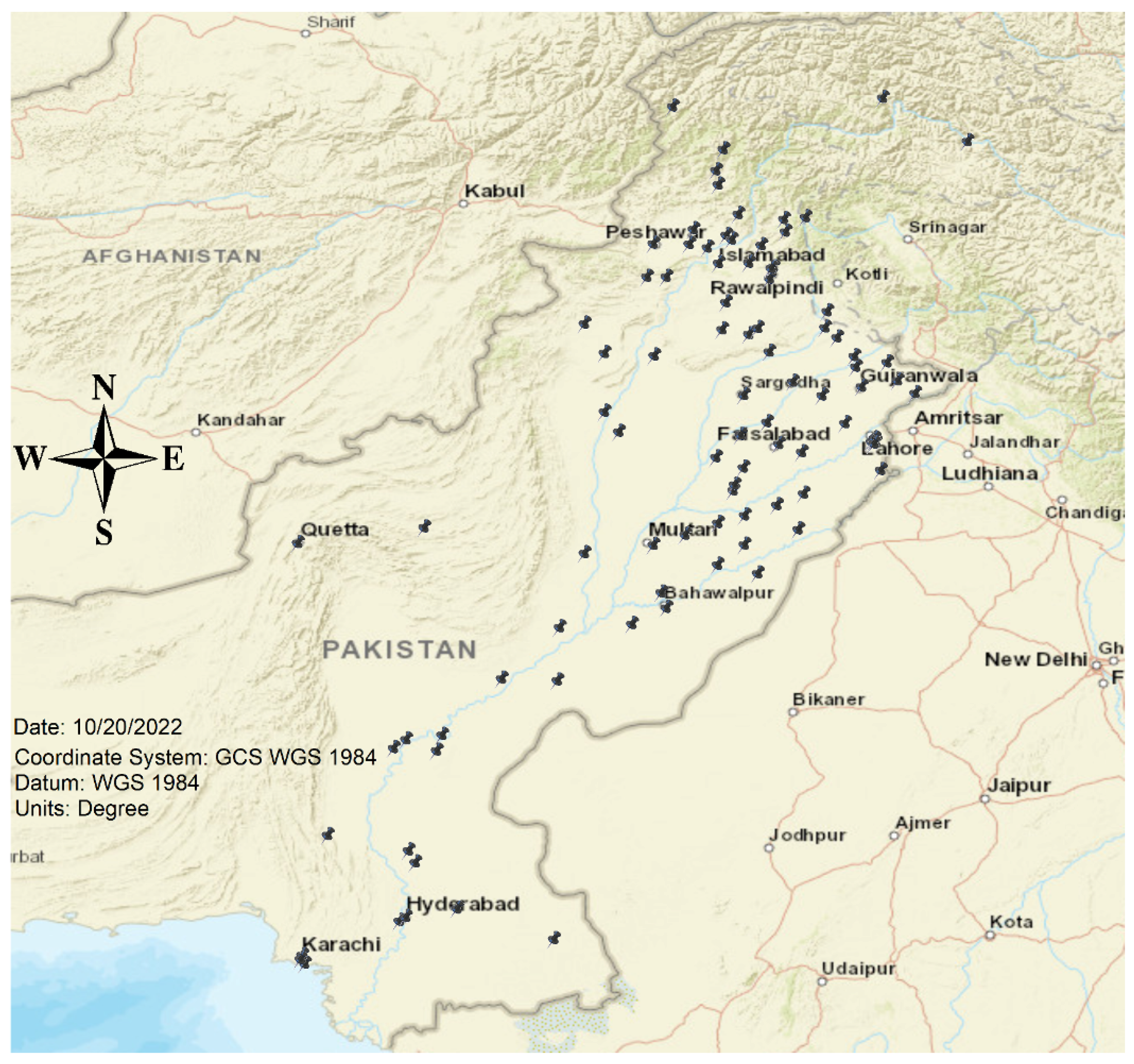
For a geospatial analysis, first, the city-level locations were converted to latitude and longitude using the Python geopy module. Using third-party geocoders and other information sources, geopy makes it simple to find the coordinate information of addresses, cities, countries, and landmarks all over the world. Figure 9 gives a visual representation and it can be seen that most of the tweets were posted from the Punjab region of Pakistan. The city-level locations were replicated as we could only retrieve city-level information from tweets; thus, one point on the map might contain hundreds of points behind it, as it was the exact location for many other instances. This could be improved by obtaining the area-level information of the tweets to map them better and predict future locations. Tweet locations were visualized in ArcMap.

6.2. Hotspot Analysis

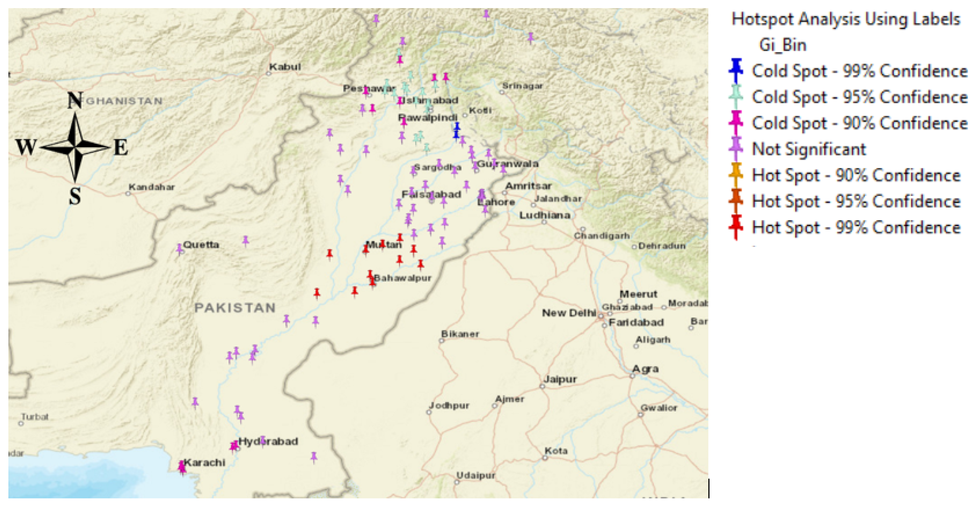
A hotspot is considered an area with a higher concentration of events than would be anticipated from a random distribution of incidents. The analysis of point distributions or spatial layouts of points in space led to the development of hotspot detection [73]. The density of locations within a given area was compared to a complete spatial randomness model, which described the point events occurring at random (i.e., a homogeneous spatial Poisson process). Hotspot techniques evaluate the level of point event interaction to comprehend spatial patterns and assess the density of data points in a particular region. The following Figure 10 visualizes the hot and cold spots that were visualized using the information from the RU-PHS labels. The legend shown on the right side gives a summary of the mapped points. The blue points show the cold spots, and the red points show the hotspots with 99% probability.

6.3. Cluster Analysis

A cluster and outlier analysis was used to validate and supplement the hotspot analysis because it could detect both groups and areas with anomalies. As a result, its findings highlighted aspects that may have been neglected in the hotspot analysis but were noteworthy, particularly in areas in which different types of subgroups coexisted. The results of this analysis (with a fixed bandwidth and a Euclidean distance of 6 miles) were very noticeable, particularly considering that the criteria were the same as in the hotspot analysis for ease of understanding and comparison purposes. Figure 11 shows the results of the cluster outlier analysis using the RU-PHS label information.

6.4. Interpolation

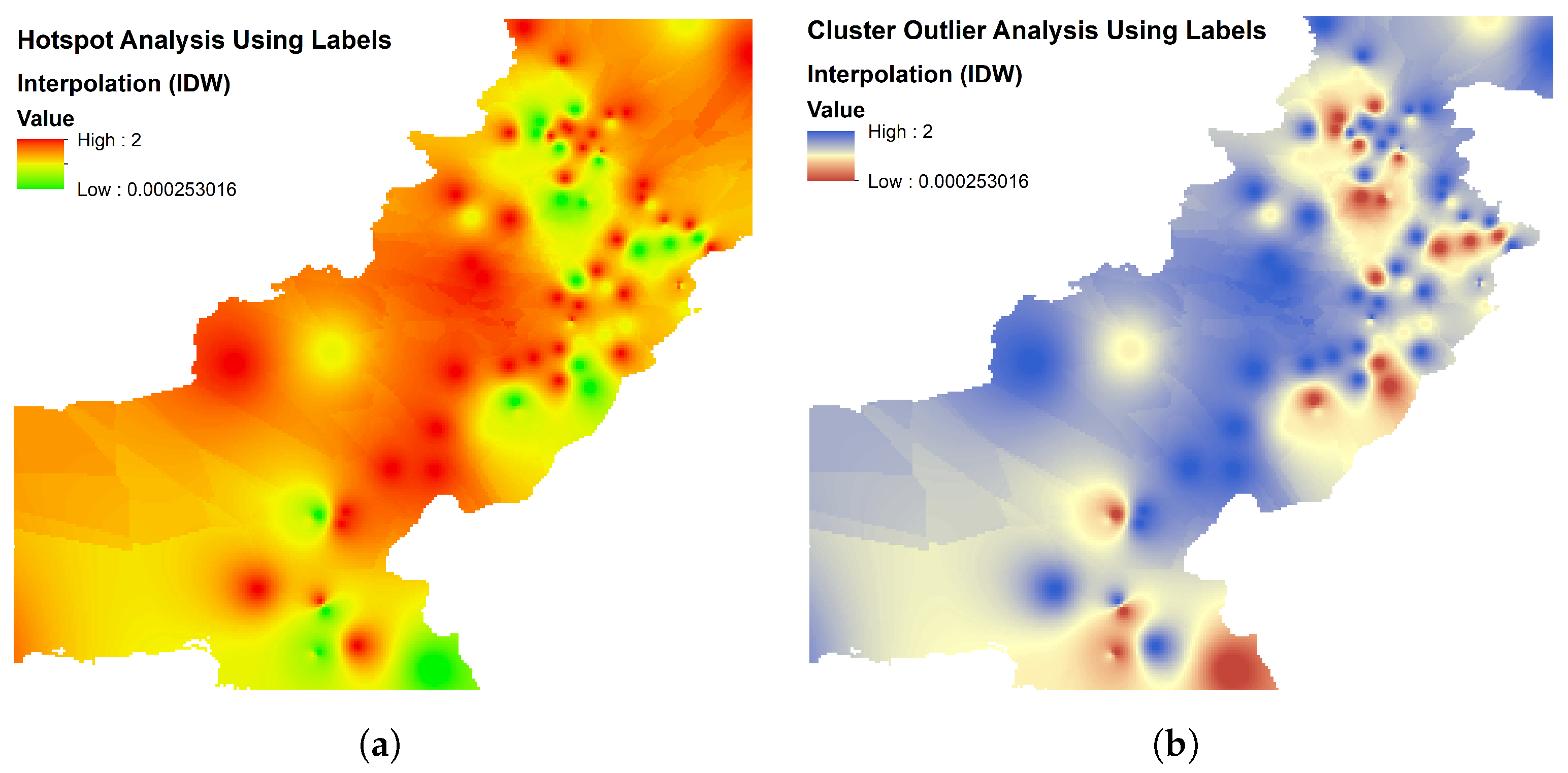
To improve visual representation and provide guidance in decision making, the results were interpolated onto a continuous surface using an inverse distance weighted interpolation (IDW), as shown in Figure 12a for hotspot point data and Figure 12b for cluster outlier point data. The interpolation estimates values for raster cells based on a small set of sample data points. It could forecast null values about any geographic point data. The interpolation was used only for the visual representation; otherwise, the real statistical analysis took place feature by data. Displaying both the surface and true results of the hotspot analysis simultaneously was an excellent way to logically portray both the statistical results and the more approachable visualization.

7. Results and Discussions

To test the effectiveness of our proposed methodology, we used the RU-PHS dataset developed and labeled by this research. Before the experiment, the data set was cleaned, lexically unified, lemmatized for English words, tokenized, and transformed by a SMOTE analysis since the data set suffered imbalance. We used TF-IDF vectorizer, word2vec, and fastText for dense vector representations of words. The aim was to classify political hate speech into three classes neutral (N), politically offensive hate (PO), and politically medium hate (PM). For the classification, conventional machine learning models were used to present a comparative analysis concerning deep neural networks.

7.1. Hyperparameters

The vocabulary size was 13,799; the input length was equal to the maximum number of tokens present in the sentence, and a low-rank projection of the co-occurrence statistics of each word concerning all other words was 50, i.e., the embedding dimension passed as the output dimension to the embedding layer. Similar embedding layer dimensions were leveraged for different vector embeddings. To experiment, the data were split into the typical 80%, 20% split, where 20% of the data were for testing and validating the proposed model. The feed-forward neural network consisted of five layers with ReLu as an activation function and softmax on the output layer to predict a multinomial probability distribution for multiclass classification. Table 8 presents the model summary of feed-forward neural network architecture for the classification of RU-PHS.
Similarly, the convolutional neural network was implemented with 723,401 trainable parameters for 15 epochs. To measure the performance of both our classification models based on error and probability, the categorical cross-entropy was used as the loss function, since it is commonly used for multiclass classification tasks. To optimize stochastic gradient descent, the Adam optimizer was used as it provides more efficient neural network weights by running repeated cycles of adaptive moment estimation. The only difference was that the sequences of word embeddings went through several convolutional operations with kernel heights and then through a ReLu activation and a 1D global max pooling operation. Finally, the maximum values of the dense layers were concatenated and passed to a fully connected classification layer with a softmax activation. A detailed summary of the convolutional neural network model for the classification of RU-PHS is presented in Table 9.

7.2. Model Training and Validation

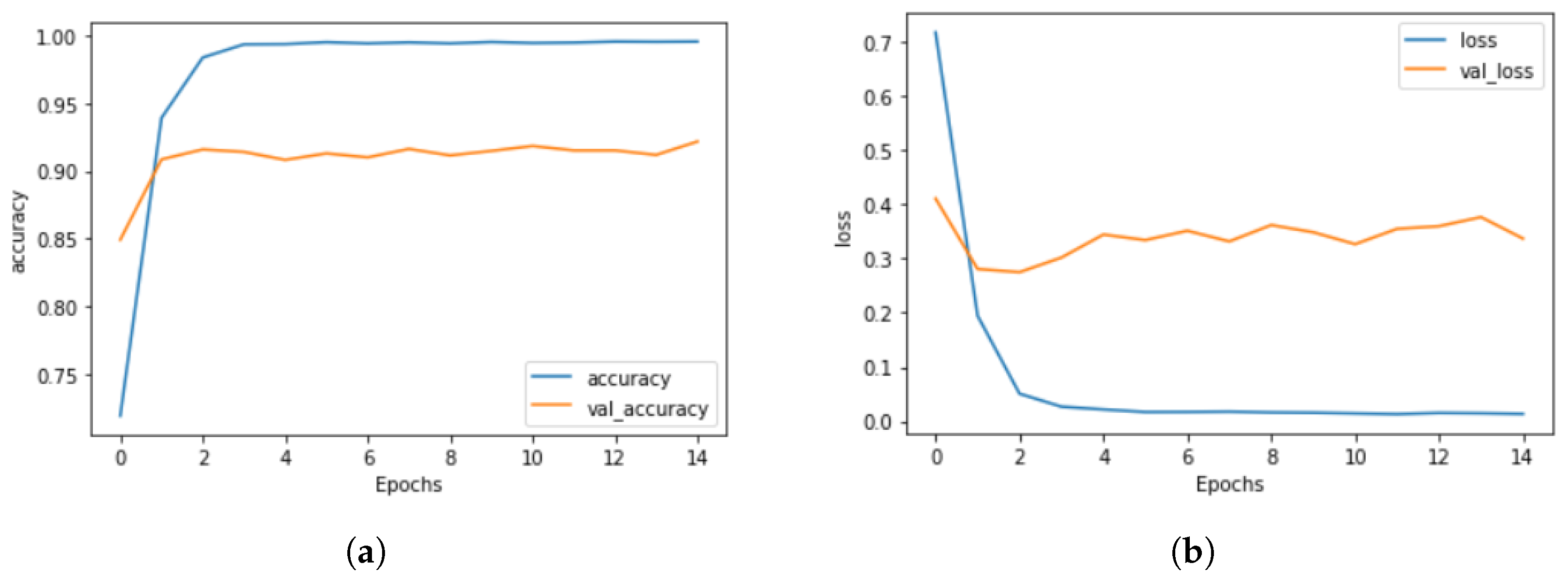
The models were trained using the training data and the accuracy was used as the evaluation metric to check models’ performance both in training accuracy and in validation accuracy. The models were trained with different numbers of epochs and the maximum validation accuracy achieved was 93% for the feed-forward neural network and 92% for the convolutional neural network for 14 epochs. Figure 13a,b gives a detailed insight into the training and validation accuracy for the feed-forward neural model with the continuous skip-gram vector representations of fastText.
The training and validation curves in Figure 14a,b indicated that increasing the training epochs could improve the precision of the CNN model. However, when we increased the number of epochs, no increment was observed in the validation accuracy; on the other hand, the training accuracy was increased to 97–98%. This suggested that the model started to overfit. Since the dataset was small and the ideal number of epochs depended on the complexity of the dataset, no improvement was seen in the model by increasing the epochs. However, it could be seen that both training and validation accuracies increased with the same trend.

7.3. Accuracy

The standard accuracy metrics were used to measure the classification performance in the RU-PHS data set, i.e., accuracy, macroaveraged precision, macroaveraged recall, macroaveraged F1 score. Since the class imbalance was tackled, to let the classifier treat each class equally and to reflect the overall performance of the model with regard to the most frequent class labels, the macroaveraged scores was used.
In this section, we compare the overall performance of conventional machine learning models and neural networks for classifying tweets into politically offensive hate, politically medium hate, and neutral classes. Table 10 shows the accuracy scores of each model about various word representations techniques. In the Table 10, it can be seen that TF-IDF performed well with conventional machine learning models such as multinomial naive Bayes with 87% accuracy, linear SVM with 89% accuracy, random forest with 91% accuracy, and gradient boosting with 90% accuracy. Since it only calculated document correlation in the word-count space rather than using a similarity score, the accuracy outcomes could be promising in this problem.
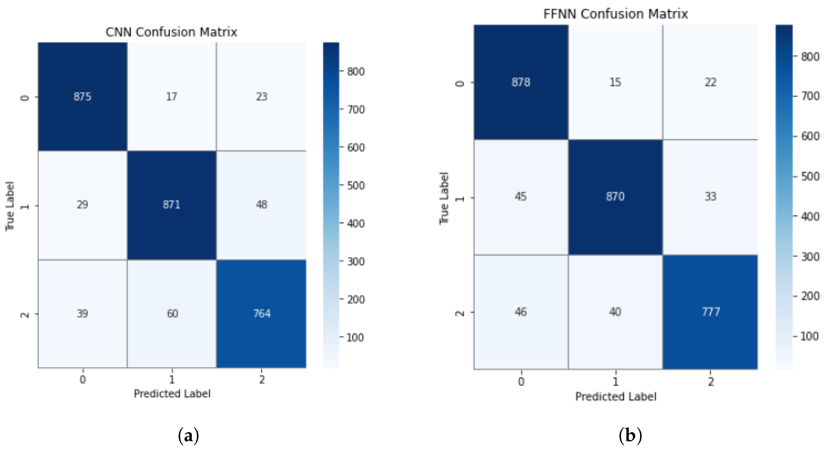
On the other hand, the continuous skip-gram model for word2vec and fastText performed really well with regression models and the proposed neural networks achieving up to 93% accuracy. Details of test classification results of each class can also be seen in the confusion matrix shown in Figure 15a,b, where 0 refers to the “neutral” class, 1 refers to the “politically medium” class and 2 refers to the “politically offensive” class. In the CNN classification for the politically offensive class Figure 15a, only 39 comments were mislabeled as neutral and 60 as politically medium, while 764 comments were classified accurately as politically offensive. For the politically medium class, 871 were correctly labeled and only 29 and 48 were mislabeled as neutral and politically offensive, respectively. For the neutral class, 875 were correctly labeled as neutral and only 17 and 23 were mislabeled as politically medium and politically offensive, respectively. Similarly, in the feed-forward NN Figure 15b classification for the politically offensive class, 777 comments were classified accurately as politically offensive. Only 40 and 46 comments were mislabeled as politically medium and neutral, respectively. For the politically medium class, 870 were correctly labeled and only 45 and 33 were mislabeled as neutral and politically offensive, respectively. For the neutral class, 878 were correctly labeled as neutral, and only 15 and 22 were mislabeled as politically medium and politically offensive, respectively.
From Table 10, it can be inferred that the proposed feed-forward neural network with the fastText continuous skip-gram model outperformed the baseline models and the convolutional neural network with a better classification convergence for the RU-PHS dataset. The time taken to build the models is presented in Table 11, and since the architecture and hyperparameters for all the classification models were different and were fine-tuned for achieving maximum accuracy, this comparison in terms of time complexity gives some insight into the results obtained and the respective time consumed.

8. Conclusions and Future Directions

This research work presented the automatic detection of political hate speech in Roman Urdu. Our significant contribution was to present an entire dataset of political hate speech from Twitter posts. The classification of Roman Urdu is challenging due to its vast lexical structure. To address this problem, we proposed an algorithm for unifying the RU-PHS dataset. In this work, we developed three different word representation techniques using TF-IDF, word2vec, and fastText to convert word-level information to vector representations. We explored the performance of seven machine learning models for the classification of the RU-PHS dataset. A comparison of the effectiveness of word representations with conventional machine learning techniques and the proposed neural networks was made. By analyzing the results from different equations, it was found that the skip-gram model of fastText, which works on character n-grams, achieved the highest empirical scores compared to word2vec, which takes into account the word n-grams. Overall, regression-based models achieved a promising accuracy but could not be considered the best approaches due to their time complexity. The proposed feed-forward neural network achieved a 93% accuracy with fastText vector representations on the RU-PHS dataset. After validation through various machine learning and deep learning methods, the dataset was mapped using the spatial information in ArcMap. The statistical information helped in the identification of trends and patterns, and the hotspot and cluster analysis assisted in pinpointing the highly susceptible areas in Pakistan. Due to a lack of resources, the information was only obtained at the city level. The results demonstrated that Punjab cities were the most affected and key locations of hate and sarcastic tweet generation.
For future work, we aim to develop a more robust algorithm for the lexical unification of Roman languages. We also consider collecting area-specific location information of tweets for a better predictability of affected regions. We also aim to train the proposed model for generic speech classification. Our dataset RU_PHS was made available for the research community to reproduce results. It will help in the development of more generic machine learning models for the detection of political hate speech in Roman Urdu.

Author Contributions

Conceptualization, S.A., M.U., M.U.A., M.S.S. and H.T.R.; methodology, S.A.; validation, M.U., M.U.A., M.S.S. and H.T.R.; formal analysis, M.U. and M.U.A.; investigation, M.U. and M.U.A.; data curation, S.A. and M.U.; writing—original draft preparation, S.A.; writing—review and editing, M.S.S., M.U., M.U.A. and H.T.R.; supervision, M.S.S. and H.T.R.; resources, M.S.S. and H.T.R. All authors have read and agreed to the published version of the manuscript.

Funding

This research received no external funding.

Data Availability Statement

The dataset shall be available through declaration from all authors.

Conflicts of Interest

The authors declare no conflict of interest.

References

  1. Gitari, N.D.; Zuping, Z.; Damien, H.; Long, J. A lexicon-based approach for hate speech detection. Int. J. Multimed. Ubiquitous Eng. 2015, 10, 215–230. [Google Scholar] [CrossRef]
  2. Aslam, S. Twitter by the Numbers: Stats, Demographics & Fun Facts. 2022. Available online: https://www.omnicoreagency.com/twitter-statistics/ (accessed on 8 June 2022).
  3. Djuric, N.; Zhou, J.; Morris, R.; Grbovic, M.; Radosavljevic, V.; Bhamidipati, N. Hate speech detection with comment embeddings. In Proceedings of the 24th International Conference on World Wide Web, Florence, Italy, 18–22 May 2015; pp. 29–30. [Google Scholar]
  4. Saeed, H.H.; Ashraf, M.H.; Kamiran, F.; Karim, A.; Calders, T. Roman Urdu toxic comment classification. Lang. Resour. Eval. 2021, 55, 971–996. [Google Scholar] [CrossRef]
  5. Naqvi, R.A.; Khan, M.A.; Malik, N.; Saqib, S.; Alyas, T.; Hussain, D. Roman Urdu news headline classification empowered with machine learning. Comput. Mater. Contin. 2020, 65, 1221–1236. [Google Scholar]
  6. Mehmood, F.; Ghani, M.U.; Ibrahim, M.A.; Shahzadi, R.; Mahmood, W.; Asim, M.N. A precisely xtreme-multi channel hybrid approach for roman urdu sentiment analysis. IEEE Access 2020, 8, 192740–192759. [Google Scholar] [CrossRef]
  7. Jiang, M.; Liang, Y.; Feng, X.; Fan, X.; Pei, Z.; Xue, Y.; Guan, R. Text classification based on deep belief network and softmax regression. Neural Comput. Appl. 2018, 29, 61–70. [Google Scholar] [CrossRef]
  8. Dulac-Arnold, G.; Denoyer, L.; Gallinari, P. Text classification: A sequential reading approach. In Proceedings of the European Conference on Information Retrieval, Stavanger, Norway, 10–14 April 2011; Springer: Berlin/Heidelberg, Germany, 2011; pp. 411–423. [Google Scholar]
  9. Bollen, J.; Gonçalves, B.; Ruan, G.; Mao, H. Happiness is assortative in online social networks. Artif. life 2011, 17, 237–251. [Google Scholar] [CrossRef] [PubMed]
  10. Khan, M.M.; Shahzad, K.; Malik, M.K. Hate speech detection in roman urdu. ACM Trans. Asian Low-Resour. Lang. Inf. Process. (TALLIP) 2021, 20, 1–19. [Google Scholar] [CrossRef]
  11. Rizwan, H.; Shakeel, M.H.; Karim, A. Hate-speech and offensive language detection in roman Urdu. In Proceedings of the 2020 Conference on Empirical Methods in Natural Language Processing (EMNLP), Online, 16–20 November 2020; pp. 2512–2522. [Google Scholar]
  12. Martins, R.; Gomes, M.; Almeida, J.J.; Novais, P.; Henriques, P. Hate speech classification in social media using emotional analysis. In Proceedings of the 2018 7th Brazilian Conference on Intelligent Systems (BRACIS), Sao Paulo, Brazil, 22–25 October 2018; pp. 61–66. [Google Scholar]
  13. Bilal, M.; Israr, H.; Shahid, M.; Khan, A. Sentiment classification of Roman-Urdu opinions using Naïve Bayesian, Decision Tree and KNN classification techniques. J. King Saud Univ.-Comput. Inf. Sci. 2016, 28, 330–344. [Google Scholar] [CrossRef]
  14. Alam, M.; Hussain, S.U. Roman-Urdu-Parl: Roman-Urdu and Urdu Parallel Corpus for Urdu Language Understanding. Trans. Asian Low-Resour. Lang. Inf. Process. 2022, 21, 1–20. [Google Scholar] [CrossRef]
  15. Younas, A.; Nasim, R.; Ali, S.; Wang, G.; Qi, F. Sentiment Analysis of Code-Mixed Roman Urdu-English Social Media Text using Deep Learning Approaches. In Proceedings of the 2020 IEEE 23rd International Conference on Computational Science and Engineering (CSE), Guangzhou, China, 29 December 2020–1 January 2021; pp. 66–71. [Google Scholar]
  16. Wasswa, H.W. The Role of Social Media in the 2013 Presidential Election Campaigns in Kenya. Ph.D. Thesis, University of Nairobi, Nairobi, Kenya, 2013. [Google Scholar]
  17. Mukund, S.; Srihari, R.K. Analyzing Urdu social media for sentiments using transfer learning with controlled translations. In Proceedings of the Second Workshop on Language in Social Media, Montreal, QC, Canada, 7 June 2012; pp. 1–8. [Google Scholar]
  18. Tehreem, T. Sentiment analysis for youtube comments in roman urdu. arXiv 2021, arXiv:2102.10075. [Google Scholar]
  19. Aimal, M.; Bakhtyar, M.; Baber, J.; Lakho, S.; Mohammad, U.; Ahmed, W.; Karim, J. Identifying negativity factors from social media text corpus using sentiment analysis method. arXiv 2021, arXiv:2107.02175. [Google Scholar]
  20. Habiba, R.; Awais, D.M.; Shoaib, D.M. A Technique to Calculate National Happiness Index by Analyzing Roman Urdu Messages Posted on Social Media. ACM Trans. Asian Low-Resour. Lang. Inf. Process. (TALLIP) 2020, 19, 1–16. [Google Scholar] [CrossRef]
  21. Hussain, A.; Arshad, M.U. An Attention Based Neural Network for Code Switching Detection: English & Roman Urdu. arXiv 2021, arXiv:2103.02252. [Google Scholar]
  22. Sadia, H.; Ullah, M.; Hussain, T.; Gul, N.; Hussain, M.F.; ul Haq, N.; Bakar, A. An efficient way of finding polarity of roman urdu reviews by using Boolean rules. Scalable Comput. Pract. Exp. 2020, 21, 277–289. [Google Scholar] [CrossRef]
  23. Rana, T.A.; Shahzadi, K.; Rana, T.; Arshad, A.; Tubishat, M. An Unsupervised Approach for Sentiment Analysis on Social Media Short Text Classification in Roman Urdu. Trans. Asian Low-Resour. Lang. Inf. Process. 2021, 21, 1–16. [Google Scholar] [CrossRef]
  24. Akhter, M.P.; Jiangbin, Z.; Naqvi, I.R.; Abdelmajeed, M.; Sadiq, M.T. Automatic detection of offensive language for urdu and roman urdu. IEEE Access 2020, 8, 91213–91226. [Google Scholar] [CrossRef]
  25. Santosh, T.; Aravind, K. Hate speech detection in hindi-english code-mixed social media text. In Proceedings of the ACM India Joint International Conference on Data Science and Management of Data, Kolkata, India, 3–5 January 2019; pp. 310–313. [Google Scholar]
  26. Arshad, M.U.; Bashir, M.F.; Majeed, A.; Shahzad, W.; Beg, M.O. Corpus for emotion detection on roman urdu. In Proceedings of the 2019 22nd International Multitopic Conference (INMIC), Islamabad, Pakistan, 29–30 November 2019; pp. 1–6. [Google Scholar]
  27. Mahmood, Z.; Safder, I.; Nawab, R.M.A.; Bukhari, F.; Nawaz, R.; Alfakeeh, A.S.; Aljohani, N.R.; Hassan, S.U. Deep sentiments in roman urdu text using recurrent convolutional neural network model. Inf. Process. Manag. 2020, 57, 102233. [Google Scholar] [CrossRef]
  28. Mehmood, K.; Essam, D.; Shafi, K.; Malik, M.K. Discriminative feature spamming technique for roman urdu sentiment analysis. IEEE Access 2019, 7, 47991–48002. [Google Scholar] [CrossRef]
  29. Mukhtar, N.; Khan, M.A. Effective lexicon-based approach for Urdu sentiment analysis. Artif. Intell. Rev. 2020, 53, 2521–2548. [Google Scholar] [CrossRef]
  30. Majeed, A.; Mujtaba, H.; Beg, M.O. Emotion detection in roman urdu text using machine learning. In Proceedings of the 35th IEEE/ACM International Conference on Automated Software Engineering Workshops, Virtual Event, Australia, 21–25 December 2020; pp. 125–130. [Google Scholar]
  31. Naqvi, U.; Majid, A.; Abbas, S.A. UTSA: Urdu text sentiment analysis using deep learning methods. IEEE Access 2021, 9, 114085–114094. [Google Scholar] [CrossRef]
  32. Chen, Y.; Zhou, Y.; Zhu, S.; Xu, H. Detecting offensive language in social media to protect adolescent online safety. In Proceedings of the 2012 International Conference on Privacy, Security, Risk and Trust and 2012 International Confernece on Social Computing, Amsterdam, The Netherlands, 3–5 September 2012; pp. 71–80. [Google Scholar]
  33. Xiang, G.; Fan, B.; Wang, L.; Hong, J.; Rose, C. Detecting offensive tweets via topical feature discovery over a large scale twitter corpus. In Proceedings of the 21st ACM International Conference on Information and Knowledge Management, Maui, HI, USA, 29 October–2 November 2012; pp. 1980–1984. [Google Scholar]
  34. Dinakar, K.; Jones, B.; Havasi, C.; Lieberman, H.; Picard, R. Common sense reasoning for detection, prevention, and mitigation of cyberbullying. ACM Trans. Interact. Intell. Syst. (TiiS) 2012, 2, 1–30. [Google Scholar] [CrossRef]
  35. Warner, W.; Hirschberg, J. Detecting hate speech on the world wide web. In Proceedings of the Second Workshop on Language in Social Media, Montreal, QC, Canada, 7 June 2012; pp. 19–26. [Google Scholar]
  36. Wadhwa, P.; Bhatia, M. Tracking on-line radicalization using investigative data mining. In Proceedings of the 2013 National Conference on Communications (NCC), New Delhi, India, 15–17 February 2013; pp. 1–5. [Google Scholar]
  37. Kwok, I.; Wang, Y. Locate the hate: Detecting tweets against blacks. In Proceedings of the Twenty-Seventh AAAI Conference on Artificial Intelligence, Bellevue, WA, USA, 14–18 July 2013. [Google Scholar]
  38. Nahar, V.; Al-Maskari, S.; Li, X.; Pang, C. Semi-supervised learning for cyberbullying detection in social networks. In Proceedings of the Australasian Database Conference, Brisbane, QLD, Australia, 14–16 July 2014; Springer: Berlin/Heidelberg, Germany, 2014; pp. 160–171. [Google Scholar]
  39. Burnap, P.; Williams, M.L. Hate speech, machine classification and statistical modelling of information flows on Twitter: Interpretation and communication for policy decision making. In Proceedings of the Internet, Policy & Politics, Oxford, UK, 26 September 2014. [Google Scholar]
  40. Agarwal, S.; Sureka, A. Using knn and svm based one-class classifier for detecting online radicalization on twitter. In Proceedings of the International Conference on Distributed Computing and Internet Technology, Bhubaneswar, India, 5–8 February 2015; Springer: Berlin/Heidelberg, Germany, 2015; pp. 431–442. [Google Scholar]
  41. Waseem, Z.; Hovy, D. Hateful symbols or hateful people? predictive features for hate speech detection on twitter. In Proceedings of the NAACL Student Research Workshop, San Diego, CA, USA, 12–17 June 2016; pp. 88–93. [Google Scholar]
  42. Di Capua, M.; Di Nardo, E.; Petrosino, A. Unsupervised cyber bullying detection in social networks. In Proceedings of the 2016 23rd International conference on pattern recognition (ICPR), Cancun, Mexico, 4–8 December 2016; pp. 432–437. [Google Scholar]
  43. Park, J.H.; Fung, P. One-step and two-step classification for abusive language detection on twitter. arXiv 2017, arXiv:1706.01206. [Google Scholar]
  44. Chen, H.; McKeever, S.; Delany, S.J. Abusive Text Detection Using Neural Networks. In Proceedings of the AICS, Dublin, Ireland, 7–8 December 2017; pp. 258–260. [Google Scholar]
  45. Badjatiya, P.; Gupta, S.; Gupta, M.; Varma, V. Deep learning for hate speech detection in tweets. In Proceedings of the 6th International Conference on World Wide Web Companion, Perth, Australia, 3–7 April 2017; pp. 759–760. [Google Scholar]
  46. Wiegand, M.; Ruppenhofer, J.; Schmidt, A.; Greenberg, C. Inducing a lexicon of abusive words–a feature-based approach. In Proceedings of the 2018 Conference of the North American Chapter of the Association for Computational Linguistics: Human Language Technologies, New Orleans, LA, USA, 1–6 June 2018; Long Papers. Association for Computational Linguistics: Cedarville, OH, USA, 2019; Volume 1, pp. 1046–1056. [Google Scholar]
  47. Pawar, R.; Agrawal, Y.; Joshi, A.; Gorrepati, R.; Raje, R.R. Cyberbullying detection system with multiple server configurations. In Proceedings of the 2018 IEEE International Conference on Electro/Information Technology (EIT), Rochester, MI, USA, 3–5 May 2018; pp. 90–95. [Google Scholar]
  48. Watanabe, H.; Bouazizi, M.; Ohtsuki, T. Hate speech on twitter: A pragmatic approach to collect hateful and offensive expressions and perform hate speech detection. IEEE Access 2018, 6, 13825–13835. [Google Scholar] [CrossRef]
  49. Malmasi, S.; Zampieri, M. Challenges in discriminating profanity from hate speech. J. Exp. Theor. Artif. Intell. 2018, 30, 187–202. [Google Scholar] [CrossRef]
  50. Pitsilis, G.K.; Ramampiaro, H.; Langseth, H. Effective hate-speech detection in Twitter data using recurrent neural networks. Appl. Intell. 2018, 48, 4730–4742. [Google Scholar] [CrossRef] [Green Version]
  51. Fernandez, M.; Alani, H. Contextual semantics for radicalisation detection on Twitter. In Proceedings of the Semantic Web for Social Good Workshop (SW4SG) at International Semantic Web Conference 2018, Monterey, CA, USA, 9 October 2018. [Google Scholar]
  52. Ousidhoum, N.; Lin, Z.; Zhang, H.; Song, Y.; Yeung, D.Y. Multilingual and multi-aspect hate speech analysis. arXiv 2019, arXiv:1908.11049. [Google Scholar]
  53. Zhang, Z.; Luo, L. Hate speech detection: A solved problem? the challenging case of long tail on twitter. Semant. Web 2019, 10, 925–945. [Google Scholar] [CrossRef]
  54. Kaur, A.; Gupta, V. N-gram based approach for opinion mining of Punjabi text. In Proceedings of the International Workshop on Multi-Disciplinary Trends in Artificial Intelligence, Bangalore, India, 8–10 December 2014; Springer: Berlin/Heidelberg, Germany, 2014; pp. 81–88. [Google Scholar]
  55. Ashari, A.; Paryudi, I.; Tjoa, A.M. Performance comparison between Naïve Bayes, decision tree and k-nearest neighbor in searching alternative design in an energy simulation tool. Int. J. Adv. Comput. Sci. Appl. (IJACSA) 2013, 4, 33–39. [Google Scholar] [CrossRef]
  56. Syed, A.Z.; Aslam, M.; Martinez-Enriquez, A.M. Lexicon based sentiment analysis of Urdu text using SentiUnits. In Proceedings of the Mexican International Conference on Artificial Intelligence, Pachuca, Mexico, 8–13 November 2010; Springer: Berlin/Heidelberg, Germany, 2010; pp. 32–43. [Google Scholar]
  57. Ghulam, H.; Zeng, F.; Li, W.; Xiao, Y. Deep learning-based sentiment analysis for roman urdu text. Procedia Comput. Sci. 2019, 147, 131–135. [Google Scholar] [CrossRef]
  58. Khan, L.; Amjad, A.; Afaq, K.M.; Chang, H.T. Deep sentiment analysis using CNN-LSTM architecture of English and Roman Urdu text shared in social media. Appl. Sci. 2022, 12, 2694. [Google Scholar] [CrossRef]
  59. Sharf, Z.; Rahman, S.U. Lexical normalization of roman Urdu text. Int. J. Comput. Sci. Netw. Secur. 2017, 17, 213–221. [Google Scholar]
  60. Sharf, Z.; Mansoor, H.A. Opinion mining in roman urdu using baseline classifiers. Int. J. Comput. Sci. Netw. Secur. 2018, 18, 156–164. [Google Scholar]
  61. Sharjeel, M.; Nawab, R.M.A.; Rayson, P. COUNTER: Corpus of Urdu news text reuse. Lang. Resour. Eval. 2017, 51, 777–803. [Google Scholar] [CrossRef]
  62. Dzakiyullah, N.R.; Hussin, B.; Saleh, C.; Handani, A.M. Comparison neural network and support vector machine for production quantity prediction. Adv. Sci. Lett. 2014, 20, 2129–2133. [Google Scholar] [CrossRef]
  63. Bose, R.; Aithal, P.; Roy, S. Sentiment analysis on the basis of tweeter comments of application of drugs by customary language toolkit and textblob opinions of distinct countries. Int. J. 2020, 8, 3684–3696. [Google Scholar]
  64. Suri, N.; Verma, T. Multilingual Sentimental Analysis on Twitter Dataset: A Review. Int. J. Adv. Comput. Sci. Appl. 2017, 10, 2789–2799. [Google Scholar]
  65. Jebaseel, A.; Kirubakaran, D.E. M-learning sentiment analysis with data mining techniques. Int. J. Comput. Sci. Telecommun. 2012, 3, 45–48. [Google Scholar]
  66. Gamallo, P.; Garcia, M. Citius: A Naive-Bayes Strategy for Sentiment Analysis on English Tweets. In Proceedings of the Semeval@Coling, Dublin, Ireland, 23–24 August 2014; pp. 171–175. [Google Scholar]
  67. Peña, A.; Mesias, J.; Patiño, A.; Carvalho, J.V.; Gomez, G.; Ibarra, K.; Bedoya, S. PANAS-TDL: A psychrometric deep learning model for characterizing sentiments of tourists against the COVID-19 pandemic on Twitter. In Advances in Tourism, Technology and Systems: Selected Papers from ICOTTS20; Springer: Berlin/Heidelberg, Germany, 2021; Volume 2, pp. 162–176. [Google Scholar]
  68. Jing, L.P.; Huang, H.K.; Shi, H.B. Improved feature selection approach TFIDF in text mining. In Proceedings of the International Conference on Machine Learning and Cybernetics, Beijing, China, 4–5 November 2002; Volume 2, pp. 944–946. [Google Scholar]
  69. Mikolov, T.; Sutskever, I.; Chen, K.; Corrado, G.S.; Dean, J. Distributed representations of words and phrases and their compositionality. Adv. Neural Inf. Process. Syst. 2013, 26, 1–9. [Google Scholar]
  70. Bojanowski, P.; Grave, E.; Joulin, A.; Mikolov, T. Enriching Word Vectors with Subword Information. Trans. Assoc. Comput. Linguist. 2017, 5, 135–146. [Google Scholar] [CrossRef] [Green Version]
  71. Zell, A. Simulation Neuronaler Netze; Addison-Wesley: Bonn, Germany, 1994; Volume 1. [Google Scholar]
  72. Johnson, R.; Zhang, T. Effective use of word order for text categorization with convolutional neural networks. arXiv 2014, arXiv:1412.1058. [Google Scholar]
  73. Chakravorty, S. Identifying crime clusters: The spatial principles. Middle States Geogr. 1995, 28, 53–58. [Google Scholar]
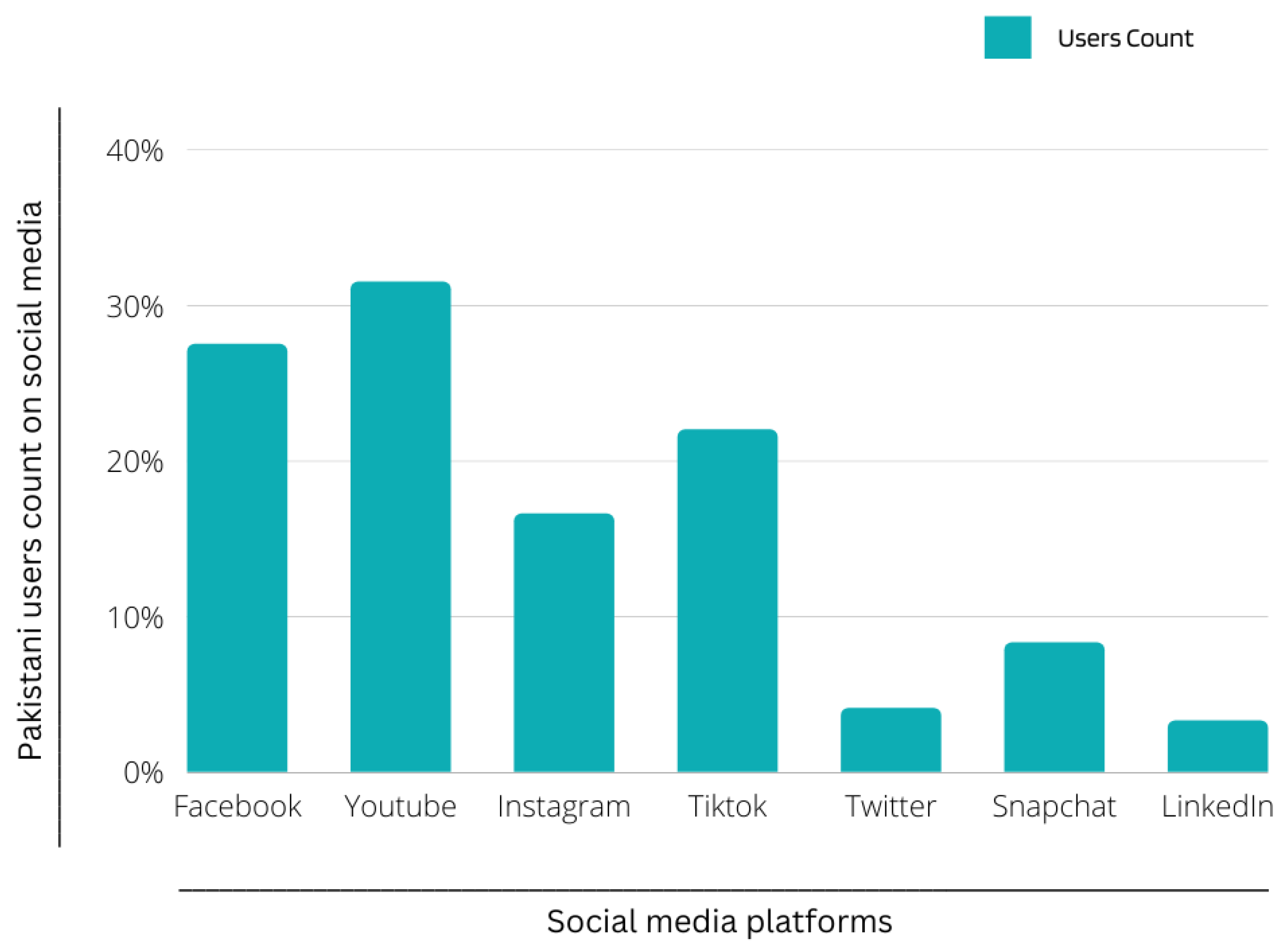
Figure 1. Active social media user stats of Pakistan based on each individual company’s ad reach in the start of 2022.
Mathematics 11 00969 g001
Figure 2. Training pipeline of text classification phenomena.
Mathematics 11 00969 g002
Figure 3. Prediction pipeline of text classification phenomena.
Mathematics 11 00969 g003
Figure 4. The representation of one-hot-encoded vectors vs. word2vec vectors.
Mathematics 11 00969 g004
Figure 5. Roman Urdu word representations using continues bag of words model of fastText.
Mathematics 11 00969 g005
Figure 6. An abstract view of proposed feed forward neural network architecture.
Mathematics 11 00969 g006
Figure 7. An abstract view of proposed 1-D convolutional neural network architecture.
Mathematics 11 00969 g007
Figure 8. Taxonomy diagram of political hate speech classification.
Mathematics 11 00969 g008
Figure 9. Visualization of city-level tweets’ information over Pakistan’s base map using ArcGIS.
Mathematics 11 00969 g009
Figure 10. Visualization of hotspot analysis of tweets’ labels over Pakistan’s base map Using ArcGIS.
Mathematics 11 00969 g010
Figure 11. Visualization of cluster outlier analysis of tweets’ labels over Pakistan’s base map using ArcGIS.
Mathematics 11 00969 g011
Figure 12. Inverse distance weighted interpolation results: (a) hotspot points data; (b) cluster outlier points data.
Mathematics 11 00969 g012
Figure 13. Accuracy and loss ROC curves of proposed feed forward neural network: (a) training and validation accuracy; (b) training and validation loss.
Mathematics 11 00969 g013
Figure 14. Accuracy and loss ROC curves of proposed convolutional neural network: (a) training and validation accuracy; (b) training and validation loss.
Mathematics 11 00969 g014
Figure 15. Confusion matrices for RU-PHS dataset classification: (a) CNN confusion matrix; (b) feed-forward NN confusion matrix.
Mathematics 11 00969 g015
Table 1. Publicly available Urdu and Roman Urdu datasets along with their characteristics.
Ref.CorpusLanguageFrequencyType
[6]DSL RU SentimentsRoman Urdu3241Sentiments
[16]RUTRoman Urdu72,000Comments
[3]HS-RU-20Roman Urdu5000Tweets
[11]RUHSOLDRoman Urdu10,012Tweets
[13]No Corpus NameRoman Urdu300Opinions
[15]MultiSentiRU and English20,735Tweets
[17]UCSAUrdu9601Reviews
[18]No Corpus NameRoman Urdu14,131YouTube Comments
[19]No Corpus NameEnglish2577Tweets
[20]No Corpus NameRoman Urdu1000Tweets
[21]Aryan UrduEnglish and RU__
[22]No Corpus NameRoman Urdu454Reviews
[23]UCI RUSA-19Roman Urdu20,229, 10,016Sentences
[24]UODUrdu RU2171YouTube Comments
[25]TRAC-1 HS HOTHindi-English12,000, 11,623Sentences
[26]RUEDRoman Urdu20,000Sentences
[27]RUSA-19Roman Urdu10,021Sentences
[28]Roman Urdu (RU)Roman Urdu11,000Reviews
[29]No Corpus NameUrdu6025Sentences
[30]No Corpus NameRoman Urdu18,000Sentences
[12]Existing DatasetEnglish24,782Tweets
[31]No Corpus NameUrdu6000Sentences
Table 2. Summary of platforms used in the collection of datasets.
Ref.TwitterYouTubeFacebookYahooFormspringWikipediaSlashdot
[3]
[32]
[33]
[34]
[35]
[36]
[37]
[38]
[39]
[40]
[41]
[42]
[43]
[44]
[45]
[46]
[47]
[48]
[49]
[50]
[51]
[52]
[53]
Table 3. Analysis of studies on the classification of Urdu and Roman Urdu hate speech.
Ref.StrengthsWeaknesses
[56]Classification of Urdu sentences
on document-level,
lexicon-based sentiment analysis
No method to tackle implicit negation
Noun phrases not considered
[57]Utilized long short-term memory
(LSTM) for polarity detection in
Roman Urdu
No validation of data collection process,
no data preprocessing method declared
Methods were not transparent
[58]806 Roman Urdu sentences collection,
feature construction, and application
on different multilingual classifiers
Limited dataset
No structure of the dataset
[59]Lexicon- and rule-based methods used to construct an RU classification algorithm, ML, and phonetic techniques usedLimited categorization of the dataset
No normalizing of the dataset
[60]15,000 roman Urdu sentences collectedThe dataset contained biographies and was not general
[31]22,000 sentences of RU were collected;
supervised and unsupervised methods were used
Ambiguous combination of classifiers
[61]1200 text documents of Urdu news were collected; performed a linguistic analysisNo character-level features used
Needs evaluation on state-of-the-art
semantic techniques
[62]Existing values collated to different techniquesNo dataset mentioned
No classification methods mentioned
[63]A massive dataset of 5 sentiments; use of lexical classifying techniquesConfusing representation of the dataset
Lack of credible results
[64]1000 reviews collected and various
frameworks compared,
i.e., Hadoop MapReduce
Limited dataset; classifiers were not general and were overfitting on the given dataset
Table 4. Word and subword decomposition example of word “Bhagora”.
RepresentationDecomposition
WordBhagora
CharacterB+h+a+g+o+r+a
Character 2-gramBh+ha+ag+go+or+ra
Character 3-gramBha+hag+ago+gor+ora
Table 5. Roman Urdu Political Hate Speech (RU-PHS) dataset characteristics.
LabelsFull Form#tweets#Words
POPolitically offensive3028273,379
PMPolitically medium119080,322
NNeutral78446,553
Table 6. The set of class guidelines developed for data labeling.
ClassesGuidelines
A tweet or phrase belonged to the “political hate speech” class if it met any or all of the following parameters:
Political hate speech  If a tweet had a hate term about a political figure, political party, government or if it targeted the followers of a specific political party. For example, “Ap ka baap nawaz bhagora chor h” translated in English as “Your father Nawaz is a truant and thief”. Some other offensive terms could be “youthia” and “patwari” targeting the supporters of specific political parties.
NeutralA tweet or phrase corresponded to the “neutral” class if it lacked any of the criteria mentioned for the political hate speech class, for example, “Wsa hi acha lgta ha mujha nawaz sharef” translated in English as “I just like nawaz sharef”.
OffensiveA tweet or phrase that belonged to the “political hate speech” class was further classified as “offensive”, if the tweet had abusive terms or symbols promoting hostility, igniting anger, or inciting harm to an individual political entity or a group of people that belonged to a political party or that supported a political profile. For example, “Bhounktey rahhooooo nawaz chor” translated in English as “Keep on barking nawaz thief”.
Medium/little offensiveA tweet or phrase that belonged to the “political hate speech” class was further classified as “sarcasm/little offensive”, if the tweet mocked and conveyed contempt against a political individual, political party, and supporter of a specific political profile yet if it did not contain explicit hate words.
For example, “Bilkul thek kaha ap nay nawaz Shareef nay boht investment ki h hmare adliya pay” translated in English as “You are right, Nawaz shareef has invested a lot in our judiciary system”.
Table 7. Words normalization using proposed lexical unification algorithm.
WordsFrequencyNormalized
Kampain74Kmpn
Kampein65Kmpn
Kampain55Kmpn
Kanpay25Knpy
Kanpein15Knpn
Kanpen12Knpn
kanpien11knpn
Table 8. Model summary of the fine-tuned feed-forward neural network.
Sr.LayerTypeOutput ShapeParametersActivation
1InputEmbedding(None, 200, 50)689,950-
2HiddenFlatten(None, 10,000)0-
3HiddenDense(None, 64)640,064ReLu
4HiddenDense(None, 32)2080ReLu
5OutputDense(None, 3)99Softmax
Table 9. Model summary of the fine-tuned convolutional neural network.
Sr.LayerTypeOutput ShapeParametersActivation
1InputEmbedding(None, 200, 50)689,950-
2HiddenConv1D(None, 196, 128)32,128Relu
3HiddenGlobalMaxPooling1D(None, 128)0-
4HiddenDense(None, 10)1290Relu
5OutputDense(None, 3)33Softmax
Table 10. Summary of results achieved by conventional machine learning approaches and proposed neural network architectures with five different word representations. The results in bold are the best results out of five feature extraction techniques in each model. For example, highest accuracy achieved by TF-IDF using Multinomial NB. Similarly in Neural Networks FastText(CSG) achieved highest accuracy out of four other feature extraction techniques.
TechniqueClassifierFeaturesAccuracy (%)Precision (%)Recall (%)F1-Score (%)
BayesMultinomial
naïve Bayes
TF-IDF
word2vec(CBOW)
word2vec(CSG)
fastText(CBOW)
fastText(CSG)
87
50
60
66
69
88
57
64
70
72
88
51
60
67
70
87
52
61
66
69
SVMLinearTF-IDF
word2vec(CBOW)
word2vec(CSG)
fastText(CBOW)
fastText(CSG)
89
62
70
74
75
90
70
75
76
77
90
73
70
74
76
90
73
70
74
77
RandomForestTF-IDF
word2vec(CBOW)
word2vec(CSG)
fastText(CBOW)
fastText(CSG)
91
88
91
91
93
92
89
92
89
92
91
89
92
91
93
91
89
92
91
93
RegressionGradient
boosting
 
TF-IDF
word2vec(CBOW)
word2vec(CSG)
fastText(CBOW)
fastText(CSG)
90
91
92
90
90
91
90
92
91
90
91
91
92
94
92
91
91
92
91
92
 XgBoost
 
TF-IDF
word2vec(CBOW)
word2vec(CSG)
fastText(CBOW)
fastText(CSG)
84
70
77
82
89
86
74
80
84
90
85
70
78
83
91
85
70
78
83
91
Neural
networks
Feed-forward
neural network
word2vec(CBOW)
word2vec(CSG)
fastText(CBOW)
fastText(CSG)
65
72
85
93
71
77
86
90
65
72
91
92
65
72
89
93
 Convolutional
neural network
word2vec(CBOW)
word2vec(CSG)
fastText(CBOW)
fastText(CSG)
70
89
85
92
75
91
88
92
71
90
89
91
71
89
89
92
Table 11. Comparison of time performance of machine learning models on RU-PHS dataset.
ClassifierMNBLSVMRFGBFFNNCNN
FeaturesTF-IDFTF-IDFfastText(CSG)W2V(CSG)fastText(CSG)fastText(CSG)
Time2 s6 s80 s60 s17 s20 s
Disclaimer/Publisher’s Note: The statements, opinions and data contained in all publications are solely those of the individual author(s) and contributor(s) and not of MDPI and/or the editor(s). MDPI and/or the editor(s) disclaim responsibility for any injury to people or property resulting from any ideas, methods, instructions or products referred to in the content.