Abstract
This paper presents an impact-angle-control guidance law with terminal constraints on the curvature of the missile trajectory. The formulation takes into account nonlinear kinematics and time-varying velocity, allowing for more general cases in which the flight path angle may not be small throughout the entire trajectory. The proposed optimal guidance law aims to minimize the change rate of pseudo-curvature, which is defined as a curvature with weighting factors based on the flight-path angle and range to go. The analysis shows that the trajectories generated by this nonlinear guidance law have a simple polynomial form with respect to downrange. Numerical simulations demonstrate that the cost function parameter can be used to shape the trajectories along the downrange.
MSC:
49-xx
1. Introduction
The impact angle or flight path angle control is significant for missiles in the initial or midcourse guidance phase to smoothly transition to the next phase, or for missiles in the terminal phase to increase terminal effectiveness. Over the past several decades, there has been extensive research on advanced guidance laws to achieve a designated impact angle, or terminal flight path angle, using optimal control theory and other methods.
Many researchers have studied various guidance laws to control the impact angle using optimal control theory, including an optimal impact angle control guidance law for re-entry vehicles [1] and for missiles with varying velocity and a maneuvering target [2], an energy-optimal impact angle control law for missiles with arbitrary dynamics [3], and a time-to-go weighted optimal impact angle control guidance law for constant speed missiles with first-order lag [4], as well as linear quadratic guidance laws for arbitrary-order linear missile dynamics [5]. Other researchers have studied optimal guidance laws with hard constraints on impact time and terminal acceleration for constant speed missiles with first-order systems and an acceleration constraint [6,7], as well as an optimal guidance law with impact-angle and acceleration constraints for an exo-atmospheric interception [8]. Except for a few studies like a nonlinear optimal impact-angle-constrained guidance with a large initial heading error [9], most of these studies based on optimal control theory have used a linear kinematics model that is linearized under the small angle assumption. Other researchers have studied various guidance laws to control the impact angle that do not rely on the optimal control framework, including biased proportional navigation guidance laws (BPNG) that add a fixed bias [10], an integral of bias [11], a time-varying bias based on relative range [12], and a shaping bias to take into account a look-angle limitation [13] to proportional navigation guidance (PNG). Sliding mode control techniques have been used for impact-angle control of maneuvering targets in some cases [14,15], and two-phase guidance schemes with terminal angle constraints have been introduced [16,17]. The time-to-go polynomial guidance law has been proposed for missile guidance with zero terminal acceleration and a specified impact angle [18,19], and a nonlinear impact angle guidance law with time-varying thrust has also been proposed [20]. Some researchers have focused on terminal acceleration constraints to improve the properties of flight trajectories driven by these impact angle control guidance laws [6,7,16,17,18,19]. A zero-terminal acceleration constraint is useful for reducing the possibility of command saturation near the target, improving the missile’s terminal performance and minimizing the angle-of-attack at the moment of impact for some missile applications [19]. However, it is also important to consider non-zero acceleration constraints, as missiles may need to achieve a non-zero acceleration at the terminal point, or handover point, for a smooth handover to a gravity-turn-type midcourse guidance phase. Therefore, there is a need for a new guidance law that can handle both zero and arbitrary terminal acceleration constraints.
Missiles generally go through a series of guidance phases, such as initial, midcourse, and terminal guidance, during their missions. These phases can sometimes involve sudden changes in velocity due to factors such as thrust, altitude changes, or stage separation. In order to shape the flight trajectory when velocity is rapidly changing, it is often more effective to tune the curvature of the trajectory rather than the acceleration. This study will, therefore, focus on the curvature as a tuning state, rather than assuming a constant speed and treating terminal acceleration or jerk as the tuning state as many previous studies have done. To achieve this aim, the constraints on acceleration will be expressed as constraints on the corresponding curvature.
In this paper, a guidance law for impact angle control with terminal constraints on the curvature of the missile trajectory is developed. The formulation takes into account nonlinear kinematics to cover more general cases in which the flight path angle cannot be assumed to be small throughout the entire trajectory, and it also accounts for time-varying velocity. Using optimal control theory, we derive an optimal guidance law that minimizes the change rate of pseudo-curvature, which is defined as a curvature with weighting factors in terms of the flight-path angle and range-to-go. The characteristics of the trajectories governed by this guidance law are analyzed, and through numerical simulations, we show that the parameters in the cost function can shape the trajectories along the downrange.
2. Problem Statement
The guidance geometry in the plane is illustrated as Figure 1. A missile at is in flight up to a goal point with a velocity and a flight path angle . Let be an acceleration normal to the velocity, which plays a role as a guidance command. Hereafter, the subscript denotes the terminal condition. The velocity of the missile changes in time due to external forces such as aerodynamic force, thrust, or gravity force.
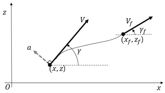
Figure 1.
Guidance geometry.
The kinematics are given by
Under the assumption that , let the independent variable be changed from to in (1)–(3). Then,
where and which is a curvature-like quantity when is small. Note that becomes a curvature exactly if is zero. Let us define a new control variable as the changing rate of pseudo-curvature with respect to the downrange as follows.
All boundary conditions of (4)–(6) are given by
where which implies a terminal curvature if the coordinate system is intentionally set as Hereafter, the subscript 0 denotes the initial condition. Note that the terminal velocity will be determined by some hidden dynamics not written here.
The problem posed here is to obtain an optimal acceleration guidance solution minimizing
where and is a non-negative integer playing a role as a shaping factor, subject to three dynamic constraints in (4)–(6) and boundary conditions in (7) and (8). Note that the performance index implies the energy-like quantity of the change rate of pseudo-curvature with respect to downrange, which is also weighted by the range-to-go function. Please remember that a unique assumption in this formulation is that , which would not be so restrictive in the application.
3. Derivation of the Optimal Guidance Law
This linear quadratic optimal control problem can be solved straightforwardly by applying Pontryagin’s principle [21]. The Hamiltonian is given by
where the co-state equations are developed as
The integration of (11)–(13) backwardly from the boundary conditions, known as the terminal transversality conditions, yields
where and are constants to be determined so as to satisfy the terminal conditions of state equations. Since the initial state has no constraint, the initial co-state is zero so that, from (16)
The extremal control is given by solving
Hence, from (16) and (18)
Substitute (19) into (6), integrate the state Equations (4)–(6) one by one, and apply the terminal conditions of (8). Then, we obtain
where each constant and is defined as, respectively, , . Since (20)–(22) have to satisfy the initial conditions of (7), the constants of are determined as
Substitution of (23)–(25) into (17) gives us
Let us consider the initial states as the current states in (26). In addition, from the definition of , the closed-loop acceleration guidance command can be obtained as
Or, by the definition of gi and gi,j,
Note that all information for guidance can be obtained from the inertial sensors. In addition, note that the guidance law does not require the estimation of time-to-go, which is needed for most of the optimal guidance laws obtained from the linearized formulation. The estimation of time-to-go is not easy itself in time-varying velocity cases. It is noteworthy that, from (22), the resultant optimal trajectories turn out to be a polynomial with an order of + 5 with respect to downrange, although the acceleration command in (27) is not a polynomial with respect to downrange.
If we set the axis so as to nullify the terminal flight path angle, then the guidance law can be simpler as
where becomes exactly a terminal curvature. Furthermore, for a zero-curvature requirement, that is, a zero acceleration at the terminal instance, the guidance command can be much simpler as
4. Numerical Simulation
In order to investigate the performance of the proposed law, let us consider a missile flying at an initial boosting-and-ascending guidance phase as shown in Figure 2. The missile is assumed to be launched vertically by a booster, which provides a propulsion force during the finite burning time. After the burnout time, the missile decelerates by aerodynamic forces and gravity forces. The objective of the initial guidance phase is to steer the missile towards a predetermined terminal position with a specific flight path angle. In Figure 2, the coordinate system describes the inertial frame with an origin at the mean sea level, and represents the guidance frame with an x-axis aligned to the desired terminal path angle. The origin of the guidance frame is positioned at a specific point to make the initial x-component equal to zero for simplicity. The missile M is launched at the origin of the inertial frame. Here, and denote the flight path angle in the guidance frame and the final flight path angle in the inertial frame, respectively. Note that T, L, and D represent thrust, lift, and drag force, respectively. The thrust force is exerted on the missile along the missile body axis during the burning time of the booster. The lift and drag forces are exerted on the missile normal to and along the velocity vector, respectively. The angle of attack is the angle between the missile body axis and the velocity vector . The gravity force is acting along the -axis.
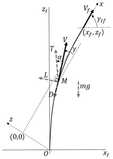
Figure 2.
Guidance geometry for simulation.
The governing equations for simulation are given by
Assume that the angle of attack is small, then and . Then, (33) and (34) become
where , , , and . denotes the reference area and is an air density, which is a function of altitude. Note that is an acceleration by an aerodynamic and thrust force, and from the comparison of (3) and (33).
For simulation, the thrust is assumed to be constant as 60,000 N for 10 s with a specific impulse of = 250 s. The missile with an initial mass of 1000 kg is assumed to be vertically launched at the origin, and the terminal aim point is at in the inertial frame. The terminal flight path angle is set to be 75 degrees. For aerodynamic forces, it is assumed that = 0.04 and = 1.2.
As previously mentioned, the main goal of this initial guidance stage is to steer the missile to the given fixed position with a designated flight path angle. Moreover, at the reaching point, the missile has to satisfy the constraint on the terminal curvature. The two cases are taken into account: first, the curvature should be zero at terminal point; second, the curvature has to achieve a given non-zero value. The terminal value is set to be zero if we want a zero acceleration at terminal instance regardless of terminal velocity, which is the most general case dealt with in lots of previous studies. In this case, the zero-curvature constraint is exactly corresponding to the zero-acceleration constraint. On the other hand, if we want to achieve a specific curvature at the terminal point, a corresponding value has to be set. As a representative example, if , then it means that the missile would achieve a flight condition at such a moment from which the missile can start off and maintain a gravity turn without any further control effort by aerodynamic or propulsive forces. In the equation, is a gravity constant and means the flight path angle in the inertial coordinate system.
4.1. First Case: Terminal Zero Curvature
In this first scenario, the terminal curvature is set to be zero, which implies that the acceleration command nullifies at the terminal point. Then, the guidance command of (29) can be employed and, as an example, the shaping factor is selected as n = 1. The simulation results in Figure 3 illustrate the performance of the proposed guidance law. Figure 3a shows that the terminal position constraint is satisfied in the inertial frame. The velocity profile with respect to time is depicted in Figure 3b. The velocity gradually decreases after it increases for 10 s by boosting thrust. The trajectory and the flight path angle profile are presented in Figure 3c,d, which indicates the terminal flight path angle constraint is satisfied and the assumption that is not violated in the whole time. The acceleration guidance command profile is presented in Figure 3e. It shows clearly that the terminal acceleration nullifies.
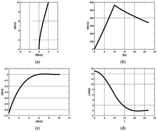
Figure 3.
First scenario. (a) Trajectory in inertial frame; (b) Velocity; (c) Trajectory in guidance frame; (d) Flight path angle; (e) Acceleration; (f) Pseudo-curvature.
4.2. Second Case: Non-Zero Curvature
In this second scenario, the acceleration command has to satisfy a gravity turn condition at the terminal point, which is a desirable handover condition to midcourse guidance for the gravity turn. This requirement is translated into the terminal curvature and has to satisfy the condition , no matter what the terminal velocity becomes. The velocity is determined by dynamics of (34), so the terminal value won’t be determined until it reaches the final time. Nonetheless, the guidance law requires from the beginning. Thus, the terminal velocity value should be estimated beforehand to set . Here, a simple way is introduced as , where . Note that denotes a roughly estimated value once at the first time, and is a current velocity. It is obvious that goes to as goes to zero. For this simulation, is set to be 300 m/s.
In the second scenario, the guidance command of (28) can be used, and for illustration purposes, the shaping factor is chosen as n = 1. The simulation results in Figure 4 illustrate the performance of the proposed guidance law associated with non-zero curvature. Figure 4a shows that the terminal position constraint is satisfied in the inertial frame. The velocity profile with respect to time and the terminal velocity estimation value are depicted in Figure 4b, respectively. The velocity gradually decreases to 340 m/s after it increases for 10 s by boosting thrust. One can also observe that the terminal velocity estimation gradually goes closer to the real value. The trajectory and the flight path angle profile are presented in Figure 4c,d, which indicates the terminal flight path angle constraint is satisfied and the assumption that is not violated the whole time. The acceleration guidance command profile is presented in Figure 4e. It shows that the terminal acceleration constraint is satisfied (−0.26 g) and, thus, the terminal curvature condition is also satisfied (−2.19 × /m).
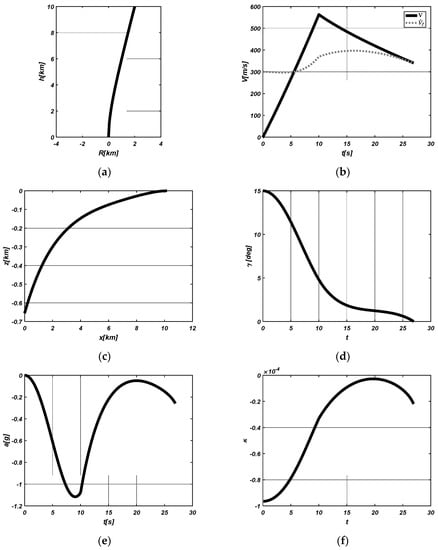
Figure 4.
Second scenario. (a) Trajectory in inertial frame; (b) Velocity; (c) Trajectory in guidance frame; (d) Flight path angle; (e) Acceleration; (f) Pseudo-curvature.
4.3. Effect of n on Trajectories
Let us take into account the effect of n on the shape of trajectories. For comparison, the same scenario as the first one is exploited except for the different shaping factors. To investigate the effect of n clearly, we take n as 0, 3, and 5, respectively. Figure 5 depicts the trajectory, the flight path angle, the acceleration, and the pseudo-curvature with respect to n. Through all figures, as expected, it is apparent that the high value of n suppresses the change of the curvature as goes to zero. Consequently the change of acceleration reduces at the terminal.
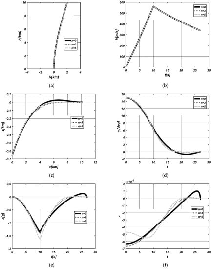
Figure 5.
Effect of n on trajectories. (a) Trajectory in inertial frame; (b) Velocity; (c) Trajectory in guidance frame; (d) Flight path angle; (e) Acceleration; (f) Pseudo-curvature.
5. Conclusions
In this paper, a new impact-angle-control guidance law that satisfies a given terminal curvature constraint is developed. The closed-form optimal guidance law, which minimizes the change rate of the pseudo-curvature, is derived. The pseudo-curvature is defined as a curvature with flight-path-angle and range-to-go weighting factors. In the derivation, we use nonlinear kinematics to cover more general cases where the flight path angle cannot be assumed to be small along the entire trajectory. This allows us to avoid some limitations associated with linearization under small angle assumptions in the application. Here, a unique assumption in the formulation is that the flight path angle must have a magnitude smaller than π/2, which would not be as restrictive in the application. In addition, we do not assume a constant speed, which is widely relied upon in previous studies. The closed-form solution is expressed in terms of velocity, the flight path angle, and the positions, all of which can be obtained from inertial sensors. The guidance law also does not require the estimation of time-to-go, which can be complicated in cases with time-varying velocity. It has been analyzed that the trajectories driven by this guidance law result in a polynomial with respect to downrange, even though the acceleration command is not a polynomial function. Numerical solutions illustrate that the obtained impact-angle-control guidance law enables us to achieve not only a zero curvature (i.e., zero acceleration), but also an arbitrary curvature constraint. We have also shown that the parameters in the cost function can shape the trajectories along the downrange. Therefore, the proposed guidance law can be applied to various trajectory shaping scenarios to adjust the impact angle and curvature.
Author Contributions
Conceptualization, K.-R.S. and I.-S.J.; methodology, I.-S.J.; software, K.-R.S.; validation, K.-R.S. and I.-S.J.; formal analysis, , K.-R.S.; investigation, I.-S.J.; resources, , K.-R.S.; data curation, , K.-R.S.; writing—original draft preparation, K.-R.S.; writing—review and editing, I.-S.J.; visualization, K.-R.S.; supervision, I.-S.J.; project administration, I.-S.J.; funding acquisition, I.-S.J. All authors have read and agreed to the published version of the manuscript.
Funding
This research received no external funding.
Data Availability Statement
Not applicable.
Conflicts of Interest
The authors declare no conflict of interest.
References
- Kim, M.; Grider, K.V. Terminal guidance for impact attitude angle constrained flight trajectories. IEEE Trans. Aerosp. Electron. Syst. 1973, 9, 852–859. [Google Scholar] [CrossRef]
- Song, T.L. Impact angle control for planar engagements. IEEE Trans. Aerosp. Electron. Syst. 1999, 35, 1439–1444. [Google Scholar] [CrossRef]
- Ryoo, C.K.; Cho, H.; Tahk, M.J. Optimal guidance laws with terminal impact angle constraint. J. Guid. Control Dyn. 2005, 28, 724–732. [Google Scholar] [CrossRef]
- Ryoo, C.K.; Cho, H.; Tahk, M.J. Time-to-go weighted optimal guidance with impact angle constraints. IEEE Trans. Aerosp. Electron. Syst. 2006, 14, 483–492. [Google Scholar]
- Shaferman, V.; Shima, T. Linear quadratic guidance laws for imposing a terminal intercept angle. J. Guid. Control Dyn. 2008, 31, 1400–1412. [Google Scholar] [CrossRef]
- Lee, Y.; Ryoo, C.; Kim, E. Optimal guidance with constraints on impact angle and terminal acceleration. In Proceedings of the AIAA Guidance Control Conference Exhibition, Austin, TX, USA, 11–14 August 2003; pp. 11–14. [Google Scholar]
- Chi, H.S.; Lee, Y.I.; Lee, C.H.; Choi, H.L. A practical optimal guidance scheme under impact angle and terminal acceleration constraints. Int. J. Aero. Space Sci. 2020, 22, 923–935. [Google Scholar] [CrossRef]
- Zhao, S.; Chen, W.; Yang, L. Optimal guidance law with impact-angle constraint and acceleration limit for exo-atmospheric interception. Aerospace 2021, 8, 358. [Google Scholar] [CrossRef]
- Li, H.; Wang, J.; He, S.; Lee, C.H. Nonlinear optimal impact-angle-constrained guidance with large initial heading error. J. Guid. Control Dyn. 2021, 44, 1663–1676. [Google Scholar] [CrossRef]
- Jeong, S.; Cho, S.; Kim, E. Angle constraint biased PNG. In Proceedings of the 2004 5th Asian Control Conference, Melbourne, Australia, 20–23 July 2004; pp. 1849–1854. [Google Scholar]
- Erer, K.; Merttopçuŏ glu, O. Indirect impact-angle-control against stationary targets using biased pure proportional navigation. J. Guid. Control Dyn. 2012, 35, 700–704. [Google Scholar] [CrossRef]
- Kim, B.; Lee, J.; Han, H. Biased PNG law for impact with angular constraint. IEEE Trans. Aerosp. Electron. Syst. 1998, 34, 277–288. [Google Scholar]
- Kim, T.; Park, B.; Tahk, M. Bias-shaping method for biased proportional navigation with terminal-angle constraint. J. Guid. Control Dyn. 2013, 36, 1810–1815. [Google Scholar] [CrossRef]
- Ratnoo, A.; Ghose, D. Impact-angle constrained interception of stationary targets. J. Guid. Control Dyn. 2008, 31, 1816–1821. [Google Scholar] [CrossRef]
- Ratnoo, A.; Ghose, D. Impact-angle constrained guidance against nonstationary nonmaneuvering targets. J. Guid. Control Dyn. 2010, 32, 269–275. [Google Scholar] [CrossRef]
- Hari, N.S.B. Impact time and angle guidance with sliding mode control. IEEE Trans. Control Syst. Technol. 2012, 6, 1436–1449. [Google Scholar]
- Kumar, S.; Rao, S.; Ghose, D. Sliding-mode guidance and control for all-aspect interceptors with terminal angle constraints. J. Guid. Control Dyn. 2012, 35, 1230–1246. [Google Scholar] [CrossRef]
- Kim, T.H.; Lee, C.H.; Tahk, M.J. Time-to-go polynomial guidance laws with terminal impact angle/acceleration constraints. IFAC Proc. Vol. 2011, 44, 3915–3919. [Google Scholar] [CrossRef]
- Lee, C.H.; Kim, T.H.; Tahk, M.J.; Whang, I.H. Polynomial guidance laws considering terminal impact angle and acceleration constraints. IEEE Trans. Aerosp. Electron. Syst. 2013, 49, 74–92. [Google Scholar] [CrossRef]
- Cho, S. Analytic solution for nonlinear impact-angle guidance law with time-varying thrust. Mathematics 2022, 10, 4034. [Google Scholar] [CrossRef]
- Bryson, A.E., Jr.; Ho, Y.C. Applied Optimal Control: Optimization, Estimation, and Control; Taylor and Francis: New York, NY, USA, 2018. [Google Scholar]
Disclaimer/Publisher’s Note: The statements, opinions and data contained in all publications are solely those of the individual author(s) and contributor(s) and not of MDPI and/or the editor(s). MDPI and/or the editor(s) disclaim responsibility for any injury to people or property resulting from any ideas, methods, instructions or products referred to in the content. |
© 2023 by the authors. Licensee MDPI, Basel, Switzerland. This article is an open access article distributed under the terms and conditions of the Creative Commons Attribution (CC BY) license (https://creativecommons.org/licenses/by/4.0/).