A New Alternative to Szeged, Mostar, and PI Polynomials—The SMP Polynomials

Abstract

Szeged-like topological indices are well-studied distance-based molecular descriptors, which include, for example, the (edge-)Szeged index, the (edge-)Mostar index, and the (vertex-)PI index. For these indices, the corresponding polynomials were also defined, i.e., the (edge-)Szeged polynomial, the Mostar polynomial, the PI polynomial, etc. It is well known that, by evaluating the first derivative of such a polynomial at $x=1$, we obtain the related topological index. The aim of this paper is to introduce and investigate a new graph polynomial of two variables, which is called the SMP polynomial, such that all three vertex versions of the above-mentioned indices can be easily calculated using this polynomial. Moreover, we also define the edge-SMP polynomial, which is the edge version of the SMP polynomial. Various properties of the new polynomials are studied on some basic families of graphs, extremal problems are considered, and several open problems are stated. Then, we focus on the Cartesian product, and we show how the (edge-)SMP polynomial of the Cartesian product of n graphs can be calculated using the (weighted) SMP polynomials of its factors.

1. Introduction and Preliminaries

Distance-based topological indices are extensively used in mathematical chemistry in order to predict physico-chemical properties of chemical compounds from the underlying molecular graph. One of the most important distance-based molecular descriptors is the well-known Wiener index [1], which is defined as the sum of distances between all pairs of vertices in a given graph. More precisely, for a connected graph G, the Wiener index $W\left(G\right)$ is calculated as

$$W\left(G\right)=\sum _{\{u,v\}\subseteq V\left(G\right)}{d}_G(u,v),$$

where $d_G(u,v)$ denotes the usual shortest path distance between vertices u and v of G. See [2] for a recent review on the Wiener index.

It is easy to see that, if T is a tree, then the Wiener index can be computed as

$$W\left(T\right)=\sum _{e=uv\in E\left(T\right)}{n}_u\left(e\right|T)n_v\left(e\right|T),$$

(1)

where $n_u\left(e\right|T)$ denotes the number of vertices of T whose distance to u is smaller than the distance to v and $n_v\left(e\right|T)$ is defined analogously. Therefore, in 1994, Gutman used the right-hand side of (1) to define the so-called Szeged index for any connected graph G [3], which turned out to be useful in various applications. As a consequence, many different variations and also edge versions of this index were considered—for example, the PI index [4], the vertex-PI index [5], the edge-Szeged index [6], the Mostar index [7], and the edge-Mostar index [8]. In particular, the Mostar index recently attracted quite a lot of attention, since it can be used as a measure of peripherality in molecular graphs and networks [9]. Note that all these indices belong to the family of Szeged-like topological indices [10].

In order to formally introduce Szeged-like topological indices, we need additional notation. Let G be a connected graph. The distance between a vertex x and an edge $e=uv$ is defined as $d_G(x,e)=min\{d_G(x,u),d_G(x,v)\}$. In addition, if $e=uv$ is any edge of G, then the following notation for the sets of vertices and edges of G will be used:

$$\begin{array}{ccc}\hfill N_u\left(e\right|G)& =& \{x\in V\left(G\right)|d_G(x,u)<d_G(x,v)\},\hfill \\ \hfill N_v\left(e\right|G)& =& \{x\in V\left(G\right)|d_G(x,v)<d_G(x,u)\},\hfill \\ \hfill N_0\left(e\right|G)& =& \{x\in V\left(G\right)|d_G(x,u)=d_G(x,v)\},\hfill \\ \hfill M_u\left(e\right|G)& =& \{f\in E\left(G\right)|d_G(u,f)<d_G(v,f)\},\hfill \\ \hfill M_v\left(e\right|G)& =& \{f\in E\left(G\right)|d_G(v,f)<d_G(u,f)\},\hfill \\ \hfill M_0\left(e\right|G)& =& \{f\in E\left(G\right)|d_G(u,f)=d_G(v,f)\}.\hfill \end{array}$$

Moreover, let

$$\begin{array}{cccccc}\hfill n_u\left(e\right|G)& =|N_u\left(e\right|G)|,\hfill & \hfill n_v\left(e\right|G)& =|N_v\left(e\right|G)|,\hfill & \hfill n_0\left(e\right|G)& =|N_0\left(e\right|G)|,\hfill \\ \hfill m_u\left(e\right|G)& =|M_u\left(e\right|G)|,\hfill & \hfill m_v\left(e\right|G)& =|M_v\left(e\right|G)|,\hfill & \hfill m_0\left(e\right|G)& =|M_0\left(e\right|G)|.\hfill \end{array}$$

Obviously, $n_u\left(e\right|G)$ represents the number of vertices of G that are closer to u than to v and $m_u\left(e\right|G)$ is the number of edges of G that are closer to u than to v.

For a connected graph G with at least one edge, we can now define the Szeged index $Sz\left(G\right)$, the Mostar index $Mo\left(G\right)$, and the vertex-PI index $P{I}_v\left(G\right)$ in the following way:

$$\begin{array}{ccc}\hfill Sz\left(G\right)& =& \sum _{e=uv\in E\left(G\right)}{n}_u\left(e\right|G)n_v\left(e\right|G),\hfill \\ \hfill Mo\left(G\right)& =& \sum _{e=uv\in E\left(G\right)}|n_u\left(e\right|G)-n_v\left(e\right|G)|,\hfill \\ \hfill P{I}_v\left(G\right)& =& \sum _{e=uv\in E\left(G\right)}\left(n_u\left(e\right|G)+n_v\left(e\right|G)\right).\hfill \end{array}$$

The edge versions of these indices are defined analogously. Below is the edge-Szeged index $S{z}_e\left(G\right)$, the edge-Mostar index $M{o}_e\left(G\right)$, and the PI index $PI\left(G\right)$:

$$\begin{array}{ccc}\hfill S{z}_e\left(G\right)& =& \sum _{e=uv\in E\left(G\right)}{m}_u\left(e\right|G)m_v\left(e\right|G),\hfill \\ \hfill M{o}_e\left(G\right)& =& \sum _{e=uv\in E\left(G\right)}|m_u\left(e\right|G)-m_v\left(e\right|G)|,\hfill \\ \hfill PI\left(G\right)& =& \sum _{e=uv\in E\left(G\right)}\left(m_u\left(e\right|G)+m_v\left(e\right|G)\right).\hfill \end{array}$$

In some cases, it is useful to consider graph polynomials related to distance-based topological indices, since such polynomials provide much more information about the topology of a given graph. The most investigated among these polynomials is the Hosoya polynomial (also called Wiener polynomial), which is closely related to the Wiener index and was introduced in 1988 by Hosoya [11]. It is well known that the Wiener index of a graph G can be computed by evaluating the first derivative of the Hosoya polynomial at $x=1$.

Similarly, graph polynomials related to Szeged-like topological indices can also be introduced—for example, the Szeged polynomial $Sz(G;x)$ [12], the edge-Szeged polynomial $S{z}_e(G;x)$ [13], the Mostar polynomial $Mo(G;x)$ [9], the edge-Mostar polynomial $M{o}_e(G;x)$, the vertex-PI polynomial $P{I}_v(G;x)$ [14], and the PI polynomial $PI(G;x)$ [15]. For a connected graph G, these polynomials are defined with the following formulas:

$$\begin{array}{cccc}\hfill Sz(G;x)& =\sum _{e=uv\in E\left(G\right)}{x}^{n_u\left(e\right|G)n_v\left(e\right|G)},\hfill & \hfill S{z}_e(G;x)& =\sum _{e=uv\in E\left(G\right)}{x}^{m_u\left(e\right|G)m_v\left(e\right|G)},\hfill \\ \hfill Mo(G;x)& =\sum _{e=uv\in E\left(G\right)}{x}^{|n_u\left(e\right|G)-n_v\left(e\right|G)|},\hfill & \hfill M{o}_e(G;x)& =\sum _{e=uv\in E\left(G\right)}{x}^{|m_u\left(e\right|G)-m_v\left(e\right|G)|},\hfill \\ \hfill P{I}_v(G;x)& =\sum _{e=uv\in E\left(G\right)}{x}^{n_u\left(e\right|G)+n_v\left(e\right|G)},\hfill & \hfill PI(G;x)& =\sum _{e=uv\in E\left(G\right)}{x}^{m_u\left(e\right|G)+m_v\left(e\right|G)}.\hfill \end{array}$$

Additional investigations on these graph polynomials can be found, for example, in [16,17,18,19,20,21,22]. Recently, several so-called root-indices of graphs were defined by using Szeged-like polynomials [23]. It is interesting that the mentioned root-indices have a higher ability to discriminate graphs than the corresponding standard indices.

Let $TI\in \{Sz,S{z}_e,Mo,M{o}_e,P{I}_v,PI\}$ be a topological index and P the corresponding graph polynomial. It is obvious that, for any connected graph G, the topological index $TI\left(G\right)$ can be calculated as the first derivative of the polynomial P at $x=1$, i.e.,

$$TI\left(G\right)=P^{\prime }(G;1).$$

The aim of this paper is to define such a graph polynomial that the Szeged index, the Mostar index, and the vertex-PI index can all be calculated by using only this one polynomial. It turns out that the mentioned goal can be achieved by introducing a polynomial of two variables, which we call the SMP polynomial. Similarly, one can also define the edge-SMP polynomial, which can be used to compute the edge-Szeged index, the edge-Mostar index, and the PI index.

The structure of the paper is the following: in the next section, we formally introduce the SMP polynomial, the edge-SMP polynomial, and also the weighted version of these polynomials. In Section 3, we investigate some basic properties of the (edge-)SMP polynomial. In particular, we focus on some basic families of graphs, trees, and extremal problems related to SMP polynomials. Moreover, several open problems are stated. Finally, in Section 4, we consider Cartesian products of graphs and provide formulas for calculating the (edge-)SMP polynomial of the Cartesian product $G=G_1\square G_2\square \cdots \square G_n$ by using the (weighted) SMP polynomials of its factors. Note that some existing results related to Szeged-like topological indices and polynomials of Cartesian products can be found in [5,12,18,24,25].

2. The SMP Polynomials

As already mentioned, we introduce a new graph polynomial of two variables, which can be used to easily compute the Szeged index, the Mostar index, and the vertex-PI index of a given graph.

In the rest of the paper, we always assume that G is a connected graph with at least one edge, although sometimes this is not specifically mentioned.

Definition 1. 

Let G be a connected graph with at least one edge. TheSMP polynomialof G, denoted as $SMP(G;x,y)$, is defined as

$$SMP(G;x,y)=\sum _{\begin{array}{c}e=uv\in E\left(G\right),\\ n_u\left(e\right)\ge n_v\left(e\right)\end{array}}{x}^{n_u\left(e\right|G)}{y}^{n_v\left(e\right|G)}.$$

The next proposition is obvious, and it shows how partial derivatives of the SMP polynomial can be applied to calculate the above-mentioned topological indices.

Proposition 1. 

If G is a connected graph, then

$$\begin{array}{ccc}\hfill Sz\left(G\right)& =& \left(\frac{\partial }{\partial x}\left(\frac{\partial }{\partial y}SMP(G;x,y)\right)\right){|}_{x=y=1},\hfill \\ \hfill Mo\left(G\right)& =& \left(\frac{\partial }{\partial x}SMP\left(G;x,\frac{1}{x}\right)\right){|}_{x=1},\hfill \\ \hfill P{I}_v\left(G\right)& =& \left(\frac{\partial }{\partial x}SMP\left(G;x,x\right)\right){|}_{x=1}.\hfill \end{array}$$

Note that the advantage of the introduced polynomial is the fact that one has to consider only one polynomial instead of three to compute three well-known molecular descriptors. In addition, by combining different operations, several other topological indices can be defined and computed from the same polynomial.

Similarly, we can introduce the edge version of the SMP polynomial, which is closely related to the edge-Szeged index, the edge-Mostar index, and the PI index.

Definition 2. 

Let G be a connected graph with at least one edge. Theedge-SMP polynomialof G, denoted as $SM{P}_e(G;x,y)$, is defined as

$$SMP(G;x,y)=\sum _{\begin{array}{c}e=uv\in E\left(G\right),\\ m_u\left(e\right)\ge m_v\left(e\right)\end{array}}{x}^{m_u\left(e\right|G)}{y}^{m_v\left(e\right|G)}.$$

The following proposition can be stated.

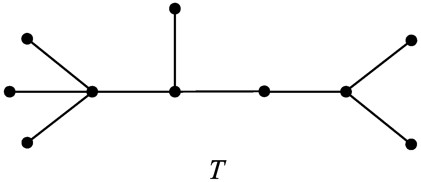
Proposition 2. 

If G is a connected graph, then

$$\begin{array}{ccc}\hfill S{z}_e\left(G\right)& =& \left(\frac{\partial }{\partial x}\left(\frac{\partial }{\partial y}SM{P}_e(G;x,y)\right)\right){|}_{x=y=1},\hfill \\ \hfill M{o}_e\left(G\right)& =& \left(\frac{\partial }{\partial x}SM{P}_e\left(G;x,\frac{1}{x}\right)\right){|}_{x=1},\hfill \\ \hfill PI\left(G\right)& =& \left(\frac{\partial }{\partial x}SM{P}_e\left(G;x,x\right)\right){|}_{x=1}.\hfill \end{array}$$

To show an example, let T be a tree from Figure 1.

Obviously, T contains six different edges $e=uv$ for which $\{n_u\left(e\right|T),n_v\left(e\right|T)\}=\{9,1\}$ and $\{m_u\left(e\right|T),m_v\left(e\right|T)\}=\{8,0\}$. Moreover, there are two edges $e=uv$ for which $\{n_u\left(e\right|T),n_v\left(e\right|T)\}=\{6,4\}$ and $\{m_u\left(e\right|T),m_v\left(e\right|T)\}=\{5,3\}$. In addition, for one edge, it holds $\{n_u\left(e\right|T),n_v\left(e\right|T)\}=\{7,3\}$ and $\{m_u\left(e\right|T),m_v\left(e\right|T)\}=\{6,2\}$. Therefore, the corresponding SMP polynomials are:

$$\begin{array}{ccc}\hfill SMP(T;x,y)& =& 6x^{9}y+x^7{y}^3+2x^6{y}^4,\hfill \\ \hfill SM{P}_e(T;x,y)& =& 6x^8+x^6{y}^2+2x^5{y}^3.\hfill \end{array}$$

It is useful to also define the weighted SMP polynomial of a graph with two weights on the edges, which will be needed in Section 4. Therefore, let G be a graph and let $w_1,w_2:E\left(G\right)\to [0,\infty )$ be two weights on the edges of G. The triple $(G,w_1,w_2)$ is then called a double edge-weighted graph.

Definition 3. 

Let $(G,w_1,w_2)$ be a double edge-weighted connected graph with at least one edge. Theweighted SMP polynomialof $(G,w_1,w_2)$, denoted as $SM{P}_{(w_1,w_2)}(G;x,y)$, is defined in the following way:

$$SM{P}_{(w_1,w_2)}(G;x,y)=\sum _{e\in E\left(G\right)}{x}^{w_1\left(e\right)}{y}^{w_2\left(e\right)}.$$

(2)

Obviously, the SMP polynomial and the edge-SMP polynomial are just special cases of the weighted SMP polynomial. More precisely, if for any edge $e=uv\in E\left(G\right)$, we define

$$n_1\left(e\right)=max\{n_u\left(e\right|G),n_v\left(e\right|G)\},n_2\left(e\right)=min\{n_u\left(e\right|G),n_v\left(e\right|G)\}$$

and

$$m_1\left(e\right)=max\{m_u\left(e\right|G),m_v\left(e\right|G)\},m_2\left(e\right)=min\{m_u\left(e\right|G),m_v\left(e\right|G)\},$$

then it holds

$$SMP(G;x,y)=SM{P}_{(n_1,n_2)}(G;x,y)\mathrm{and}SM{P}_e(G;x,y)=SM{P}_{(m_1,m_2)}(G;x,y).$$

3. Basic Properties of SMP Polynomials

In this section, several properties of SMP polynomials are discussed. We start with the following observation related to bipartite graphs.

Proposition 3. 

Let G be a connected graph on n vertices, where $n\ge 2$. Then, G is bipartite if and only if, in every term $a_{i,j}{x}^i{y}^j$ of $SMP(G;x,y)$, we have $i+j=n$.

Proof. 

Let $e=uv$ be an edge of G. If G is bipartite, then, for every vertex w, we have $d_G(u,w)\ne d_G(v,w)$, which means that $n_u\left(e\right|G)+n_v\left(e\right|G)=n$.

On the other hand, if G is non-bipartite, let C be a shortest odd cycle in G. Observe that, if $u,v\in V\left(C\right)$, then $d_G(u,v)=d_C(u,v)$; otherwise, G has an odd cycle which is shorter than C. Let $e=u_1{u}_2$ be an edge in C and let w be a vertex on C opposite to e. Then, $d_C(u,w)=d_C(v,w)$ and consequently $d_G(u,w)=d_G(v,w)$, which means that $n_u\left(e\right|G)+n_v\left(e\right|G)\le n-1$.  □

Now, we focus on trees and firstly provide the relation between the SMP polynomial and the edge-SMP polynomial in this class of graphs.

Proposition 4. 

If T is a tree, then $SM{P}_e(T;x,y)=\frac{1}{xy}SMP(T;x,y)$.

Proof. 

Let $e=uv$ be an edge of T. For every other edge $e^{\prime }=u^{\prime }{v}^{\prime }$, denote by $w_{e^{\prime }}$ that vertex from $u^{\prime }$ and $v^{\prime }$, which has a bigger distance from e. Since T is a tree, $w_{e^{\prime }}$ is defined uniquely. Then, $N_u\left(e\right|T)$ contains the vertices $\left\{w_{e^{\prime }}\right|e^{\prime }\in M_u\left(e\right|T)\}\cup \left\{u\right\}$ and $N_v\left(e\right|T)$ contains the vertices $\left\{w_{e^{\prime }}\right|e^{\prime }\in M_v\left(e\right|T)\}\cup \left\{v\right\}$. Therefore, $n_u\left(e\right|T)=m_u\left(e\right|T)+1$ and $n_v\left(e\right|T)=m_v\left(e\right|T)+1$, and consequently $SM{P}_e(T;x,y)=\frac{1}{xy}SMP(T;x,y)$.  □

Hence, for trees, it suffices to consider $SMP(T;x,y)$.

By definition, $SMP(G;1,1)$ equals the number of edges in G. Since the only connected graphs with n vertices and $n-1$ edges are trees, we have the following observation.

Observation 1. 

Let G be a connected graph on n vertices. Then, G is a tree if and only if $SMP(G;1,1)=n-1$.

Next, some special families of trees are considered. As usual, by $P_n$ and $S_n$, we denote a path and a star, respectively, on n vertices. Take an edge e. Attach a pendant edges to one endvertex of e and attach b pendant vertices to the other endvertex of e, where $a\ge b$. The resulting graph is called a double star, and it is denoted by $D_{a,b}$. Observe that $D_{a,b}$ has $a+b+2$ vertices. We have

$$\begin{array}{cc}\hfill SMP(P_n,x,y)& =\left\{\begin{array}{c}2\sum _{i=1}^{n/2-1}{x}^{n-i}{y}^i+x^{n/2}{y}^{n/2}\mathrm{if}n\mathrm{is}\mathrm{even},\hfill \\ 2\sum _{i=1}^{(n-1)/2}{x}^{n-i}{y}^i\mathrm{if}n\mathrm{is}\mathrm{odd};\hfill \end{array}\right.\hfill \\ \hfill SMP(S_n,x,y)& =(n-1)x^{n-1}y;\hfill \\ \hfill SMP(D_{a,b},x,y)& =(a+b)x^{a+b+1}y+x^{a+1}{y}^{b+1}.\hfill \end{array}$$

We can prove the next statement related to the uniqueness of the SMP polynomial.

Proposition 5. 

Let $T\in \{P_n,S_n,D_{a,b}\}$ and let $P(x,y)=SMP(T;x,y)$. Then, the unique connected graph with polynomial $P(x,y)$ is T.

Proof. 

Let $SMP(G;x,y)=P(x,y)$. Then, G has $m=P(1,1)$ edges. Consider one term of $P(x,y)$, say $a_{i,j}{x}^i{y}^j$. Then, G contains an edge (in fact, it contains at least $a_{i,j}$ edges), which is in a component with at least $i+j$ vertices. By Proposition 3 and Observation 1, $i+j=m+1$. Hence, all edges are in a single component, and G is a tree.

Denote $n=m+1$. If $e=uv$ is a pendant edge of a tree, then $\{n_u\left(e\right|G),n_v\left(e\right|G)\}=\{n-1,1\}$, and if e is not pendant, then $\{n_u\left(e\right|G),n_v\left(e\right|G)\}=\{i,j\}$, where $2\le i,j\le n-2$. Hence, $P(x,y)$ contains a term $q{x}^{n-1}y$, and q is the number of pendant edges in G. Consequently, G has q pendant vertices, which solve the cases $T\in \{P_n,S_n\}$.

In the last case, $q=n-2$. Hence, the tree G contains $n-2$ pendant edges and one edge, say f, which is not pendant. Let $x^i{y}^j$ be the term of $P(x,y)$ for which $2\le i,j\le n-2$. Then, to one endvertex of e, there are attached $i-1$ pendant vertices and, to the other endvertex of e, there are attached $j-1$ pendant vertices. Thus, T is $D_{i-1,j-1}$.  □

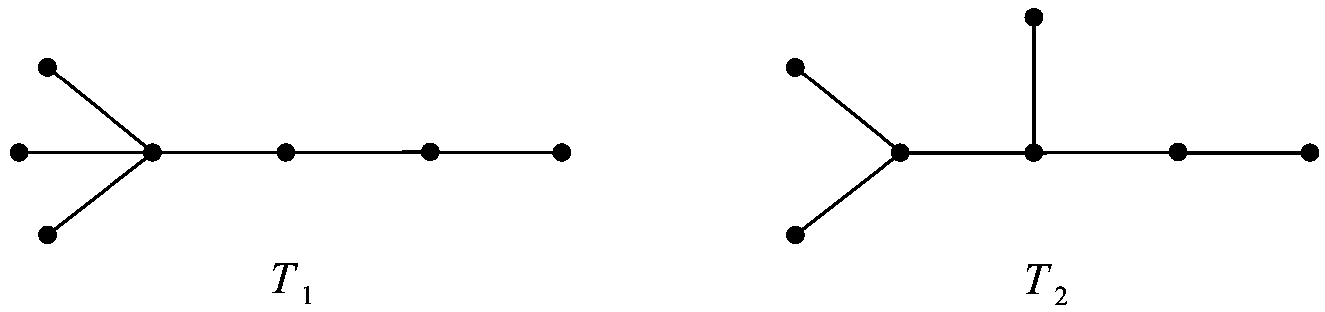
It is also interesting to investigate trees with the same SMP polynomials. One can check that the smallest nonisomorphic trees $T_1$ and $T_2$, for which $SMP(T_1;x,y)$ $=SMP(T_2;x,y)$, have seven vertices and four pendant edges; see Figure 2. More precisely, $SMP(T_1;x,y)=SMP(T_2;x,y)=4x^{6}y+x^5{y}^2+x^4{y}^3$. Note also that there exist 11 nonisomorphic trees on seven vertices, but only $T_1$ and $T_2$ have the same SMP polynomials.

Now, we consider graphs which are not trees. By $C_n$, $K_n$ and $K_{n_1,n_2}$, we denote a cycle, a complete graph and a complete bipartite graph, respectively, on n vertices. In the last case, $n=n_1+n_2$, and we also assume $n_1\ge n_2$. We have

$$\begin{array}{cc}\hfill SMP(C_n;x,y)& =n{x}^{n/2}{y}^{n/2}\mathrm{and}SM{P}_e(C_n;x,y)=n{x}^{(n-2)/2}{y}^{(n-2)/2}\mathrm{if}n\mathrm{is}\mathrm{even};\hfill \\ \hfill SMP(C_n;x,y)& =n{x}^{(n-1)/2}{y}^{(n-1)/2}\mathrm{and}SM{P}_e(C_n;x,y)=n{x}^{(n-1)/2}{y}^{(n-1)/2}\mathrm{if}n\mathrm{is}\mathrm{odd};\hfill \\ \hfill SMP(K_n;x,y)& =\left(\genfrac{}{}{0pt}{}{n}{2}\right)xy\mathrm{and}SM{P}_e(K_n;x,y)=\left(\genfrac{}{}{0pt}{}{n}{2}\right)x^{n-2}{y}^{n-2};\hfill \\ \hfill SMP(K_{n_1,n_2};x,y)& =n_1{n}_2{x}^{n_1}{y}^{n_2}\mathrm{and}SM{P}_e(K_{n_1,n_2};x,y)=n_1{n}_2{x}^{n_1-1}{y}^{n_2-1}.\hfill \end{array}$$

The case of odd cycles opens the following:

Problem 1. 

Characterize graphs G, for which $SMP(G;x,y)=SM{P}_e(G;x,y)$.

If a graph G is edge-transitive on m edges, then there are $i_1$, $j_1$ and $i_2$, $j_2$, such that $SMP(G;x,y)=m{x}^{i_1}{y}^{j_1}$ and $SM{P}_e(G;x,y)=m{x}^{i_2}{y}^{j_2}$. For example, let $O_3$ be the Petersen graph and let $Q_t$ be the graph of t-dimensional cube. Observe that $Q_t$ has $2^t$ vertices and $t{2}^{t-1}$ edges. We have

$$\begin{array}{cc}\hfill SMP(O_3;x,y)& =15x^2{y}^2\mathrm{and}SM{P}_e(O_3;x,y)=15x^6{y}^6;\hfill \\ \hfill SMP(Q_t;x,y)& =t{2}^{t-1}{x}^{2^{t-1}}{y}^{2^{t-1}}\mathrm{and}SM{P}_e(Q_t;x,y)=t{2}^{t-1}{x}^{(t-1)2^{t-2}}{y}^{(t-1)2^{t-2}}.\hfill \end{array}$$

If G is edge-transitive, then there are integers i and j (not necessarily positive), such that $SM{P}_e(G;x,y)/SMP(G;x,y)=x^i{y}^j$. Denote $\phi \left(G\right)=i+j$.

Observe that $\phi \left(K_n\right)=2n-6$ and $\phi \left(K_{n_1,n_2}\right)=-2$, while, for even n, we also have $\phi \left(C_n\right)=-2$. Moreover, $\phi \left(O_3\right)=8$ and $\phi \left(Q_t\right)=2^{t-1}(t-3)$. It would be interesting to find extremal values of $\phi$. Therefore, we state the following problem:

Problem 2. 

Characterize edge-transitive graphs on n vertices with an extremal value of φ.

Moreover, what are the graphs with the second or third extremal value of $\phi$?

Next, we consider bounds for the degree of $SMP$ and $SM{P}_e$. We set

$$\begin{array}{cc}\hfill n\left(G\right)& =max\{n_u\left(e\right|G)+n_v\left(e\right|G)|e=uv\in E\left(G\right)\},\hfill \\ \hfill m\left(G\right)& =max\{m_u\left(e\right|G)+m_v\left(e\right|G)|e=uv\in E\left(G\right)\}.\hfill \end{array}$$

Observe that $n\left(G\right)$ is the degree of $SMP(G;x,y)$, and $m\left(G\right)$ is the degree of $SM{P}_e(G;x,y)$.

In the next statement, we bound the degree of $SMP(G;x,y)$.

Proposition 6. 

Let G be a connected graph on n vertices, where $n\ge 2$.

-

If $n\left(G\right)$ is maximum possible, then $n\left(G\right)=n$, and extremal graphs include all bipartite graphs and graphs having a bridge.

-

If $n\left(G\right)$ is minimum possible, then $n\left(G\right)=2$, and G is the complete graph $K_n$.

Proof. 

First, we consider the upper bound. For every edge $e=uv$, we have $n_u\left(e\right|G)+n_v\left(e\right|G)\le n$, which means that $n\left(G\right)\le n$. By Proposition 3, if $e=uv$ is an edge of a bipartite graph, then $n_u\left(e\right|G)+n_v\left(e\right|G)=n$ and so $n\left(G\right)=n$ if G is bipartite. The same is true if e is a bridge, and so, if G is a graph with a bridge, then $n\left(G\right)=n$ as well.

Now, we consider the lower bound. For every edge $e=uv$, we have $n_u\left(e\right|G)\ge 1$ since $0=d(u,u)<d(v,u)=1$. By symmetry, also $n_v\left(e\right|G)\ge 1$, and so $n_u\left(e\right|G)+n_v\left(e\right|G)\ge 2$. If $n_u\left(e\right|G)+n_v\left(e\right|G)=2$, then every neighbour of u (other then v) must be a neighbour of v, and every neighbour of v (other than u) must be a neighbour of u. Consequently, if $n\left(G\right)=2$, then every pair $x,y$ of adjacent vertices must have the same neighbours in $V\left(G\right)\backslash \{x,y\}$. Hence, G is the complete graph $K_n$.  □

Take a complete graph on $n-1$ vertices $K_{n-1}$, attach a pendant vertex to one of the vertices of $K_{n-1}$, and denote the resulting graph by $K_{n-1}^{+}$. In the following theorem, we give a tight upper bound for the degree of $SM{P}_e(G;x,y)$.

Theorem 1. 

Let G be a connected graph on n vertices, $n\ge 2$, for which $m\left(G\right)$ is maximum possible. Then, $m\left(G\right)=\left(\genfrac{}{}{0pt}{}{n-1}{2}\right)$ if $n\ge 5$ and $m\left(G\right)=2n-4$ if $n\le 5$. Moreover, if $n\ge 6$, then $K_{n-1}^{+}$ is the unique extremal graph.

Proof. 

Let $e=uv$ be an edge, such that $m_u\left(e\right|G)+m_v\left(e\right|G)=m\left(G\right)$. If $deg\left(u\right)=deg\left(v\right)=n-1$, then every edge which is not adjacent to e has distance 1 from both u and v. Hence, $m\left(G\right)=2n-4$ since $d(u,e)=d(v,e)$.

In the following, we may assume that $n>2$ and $deg\left(v\right)<n-1$. Thus, there is a vertex, say w, which is not adjacent to v. Let x be a vertex of $V\left(G\right)\backslash \{u,v,w\}$. We consider possible edges $ux$, $vx$ and $wx$. If $ux,vx\in E\left(G\right)$, then $d(u,wx)=d(v,wx)=1$, so at most two edges from $\{ux,vx,wx\}$ contribute to $m_u\left(e\right|G)+m_v\left(e\right|G)$. Since for $x,y\in V\left(G\right)\backslash \{u,v,w\}$, where $x\ne y$, the sets $\{ux,vx,wx\}$ and $\{uy,vy,wy\}$ are disjoint, e does not contribute to $m_u\left(e\right|G)+m_v\left(e\right|G)$, and $vw\notin E\left(G\right)$, we have

$$m\left(G\right)\le \left(\genfrac{}{}{0pt}{}{n}{2}\right)-(n-3)-1-1=\left(\genfrac{}{}{0pt}{}{n-1}{2}\right).$$

However, if $e^{\prime }=u^{\prime }{v}^{\prime }$ is the pendant edge of $K_{n-1}^{+}$, then $m_{u^{\prime }}\left(e^{\prime }\right|K_{n-1}^{+})+m_{v^{\prime }}\left(e^{\prime }\right|K_{n-1}^{+})=\left(\genfrac{}{}{0pt}{}{n-1}{2}\right)$. Since $\left(\genfrac{}{}{0pt}{}{n-1}{2}\right)>2n-4$ if $n\ge 6$ (observe that equality holds if $n=5$), we have $m\left(G\right)=\left(\genfrac{}{}{0pt}{}{n-1}{2}\right)$ if $n\ge 6$ and $m\left(G\right)=2n-4$, otherwise.

Now assume that $n\ge 6$ and G is an extremal graph. As explained above, $m\left(G\right)$ is attained on $e=uv$ for which $deg\left(v\right)<n-1$. Thus, there is $w\in V\left(G\right)$ such that $vw\notin E\left(G\right)$. Moreover, G contains all edges which have both endvertices in $V\left(G\right)\backslash \{u,v,w\}$ and also $uw$.

Suppose that there is $x\in V\left(G\right)\backslash \{u,v,w\}$, such that $vx\in E\left(G\right)$. Since $n\ge 6$, there is a vertex $y\in V\left(G\right)\backslash \{u,v,w,x\}$. As mentioned above, $xy\in E\left(G\right)$ and $xy$ contributes to $m_u\left(e\right|G)+m_v\left(e\right|G)$. Since $d(v,xy)=1$, we have $ux\notin E\left(G\right)$. However, two edges from the triple $\{ux,vx,wx\}$ must contribute to $m_u\left(e\right|G)+m_v\left(e\right|G)$, and so $wx\in E\left(G\right)$. Since $uw,vx\in E\left(G\right)$, we have $d(u,wx)=d(v,wx)$ and so $wx$ cannot contribute to $m_u\left(e\right)+m_v\left(e\right)$, a contradiction. Hence, $vx\notin E\left(G\right)$ for $x\ne u$ and consequently G is $K_{n-1}^{+}$.  □

Since we do not know a tight lower bound for the degree of $SM{P}_e(G;x,y)$, we have the following problem.

Problem 3. 

Find a tight lower bound for $m\left(G\right)$ and characterize the extremal graphs.

In some chemical applications, it is interesting to consider a polynomial of (molecular) graphs for particular values of x any y, since in this way it is possible to obtain a molecular descriptor from the polynomial. For an example, see [26]. Therefore, we finish this section with the next open problem.

Problem 4. 

Characterize graphs with extremal value of $SMP(G;c_1,c_2)$ or $SM{P}_e(G;c_1,c_2)$ for a given pair $(c_1,c_2)$.

4. SMP Polynomials of Cartesian Products

In this section, we investigate the SMP polynomial and the edge-SMP polynomial of Cartesian products of graphs. First, we present some basic definitions from [27].

The Cartesian product of graphs $G_1,G_2,\dots ,G_n$ is the graph $G=G_1\square G_2\square \cdots \square G_n$ such that:

• $V\left(G\right)=V\left(G_1\right)\times V\left(G_2\right)\times \cdots \times V\left(G_n\right)$,
• two vertices $a=(a_1,a_2,\dots ,a_n)$, $b=(b_1,b_2,\dots ,b_n)\in V\left(G\right)$ are adjacent in G if and only if there exists exactly one $k\in \{1,\dots ,n\}$ such that $a_k{b}_k\in E\left(G_k\right)$ and $a_i=b_i$ for every $i\in \{1,\dots ,n\}\backslash \left\{k\right\}$.

For a vertex x of the Cartesian product G, the k-th coordinate of x will be denoted as $x_k$ for any $k\in \{1,\dots ,n\}$, i.e., $x=(x_1,x_2,\dots ,x_n)$.

In addition, for the Cartesian product $G=G_1\square G_2\square \cdots \square G_n$ and $k\in \{1,\dots ,n\}$, we use the following notation:

$$E_k\left(G\right)=\{uv\in E\left(G\right)|u_k{v}_k\in E\left(G_k\right)\}.$$

Observe that the sets $E_1\left(G\right),E_2\left(G\right),\dots ,E_n\left(G\right)$ are pairwise disjoint and

$$E\left(G\right)=E_1\left(G\right)\cup E_2\left(G\right)\cup \cdots \cup E_n\left(G\right).$$

(3)

It is well known that the Cartesian product G is connected if and only if all the factors $G_k$, $k\in \{1,\dots ,n\}$, are connected. Moreover, for vertices $a,b\in V\left(G\right)$, the following distance formula holds true [27]:

$$d_G(a,b)=\sum _{k=1}^n{d}_{G_k}(a_k,b_k).$$

(4)

We denote $r=\left|V\right(G\left)\right|$ and $s=\left|E\right(G\left)\right|$, where $G=G_1\square G_2\square \cdots \square G_n$ is the Cartesian product. In addition, let $r_k=\left|V\left(G_k\right)\right|$ and $s_k=\left|E\left(G_k\right)\right|$ for any $k\in \{1,\dots ,n\}$. Obviously, we have

$$r=\left|V\left(G\right)\right|=\prod _{k=1}^n\left|V\left(G_k\right)\right|=r_1{r}_2\cdots r_n.$$

(5)

In addition, since

$$|E_k\left(G\right)|=|E\left(G_k\right)|·\prod _{\begin{array}{c}i=1\\ i\ne k\end{array}}^n\left|V\left(G_i\right)\right|=s_k\frac{r}{r_k},$$

from Equation (3) one can obtain

$$s=\left|E\left(G\right)\right|=\sum _{k=1}^n\left|E_k\left(G\right)\right|=r\sum _{k=1}^n\frac{s_k}{r_k}.$$

(6)

Moreover, for $k\in \{1,\dots ,n\}$, we use the following notation:

$$G/G_k=G_1\square \cdots \square G_{k-1}\square G_{k+1}\square \cdots \square G_n.$$

As a consequence, by using Equations (5) and (6), we also have

$$|V(G/G_k)|=\frac{r}{r_k}\mathrm{and}\left|E(G/G_k)\right|=\frac{r}{r_k}\sum _{\begin{array}{c}i=1\\ i\ne k\end{array}}^n\frac{s_i}{r_i}.$$

(7)

Next, we investigate some subsets of vertices in Cartesian products of graphs in order to calculate the SMP polynomial.

Proposition 7. 

Suppose that $G=G_1\square G_2\square \cdots \square G_n$ is the Cartesian product of connected graphs $G_1,G_2,\dots ,G_n$. Moreover, let $k\in \{1,\dots ,n\}$ and let $f=uv$ be an edge of G such that $e=u_k{v}_k\in E\left(G_k\right)$. Then,

$$\begin{array}{ccc}\hfill N_u\left(f\right|G)& =& \{x\in V\left(G\right)|x_k\in N_{u_k}\left(e\right|G_k)\},\hfill \\ \hfill N_v\left(f\right|G)& =& \{x\in V\left(G\right)|x_k\in N_{v_k}\left(e\right|G_k)\},\hfill \\ \hfill N_0\left(f\right|G)& =& \{x\in V\left(G\right)|x_k\in N_0\left(e\right|G_k)\}.\hfill \end{array}$$

Proof. 

First, we introduce the following notation:

$$\begin{array}{ccc}\hfill A& =& \{x\in V\left(G\right)|x_k\in N_{u_k}\left(e\right|G_k)\},\hfill \\ \hfill B& =& \{x\in V\left(G\right)|x_k\in N_{v_k}\left(e\right|G_k)\},\hfill \\ \hfill C& =& \{x\in V\left(G\right)|x_k\in N_0\left(e\right|G_k)\}.\hfill \end{array}$$

We now prove that $A\subseteq N_u\left(f\right|G)$. Therefore, let $x\in A$. By (4), we know that

$$d_G(x,u)=\sum _{i=1}^n{d}_{G_i}(x_i,u_i)\mathrm{and}{d}_G(x,v)=\sum _{i=1}^n{d}_{G_i}(x_i,v_i).$$

However, $u_i=v_i$ for any $i\in \{1,\dots ,n\}\backslash \left\{k\right\}$. Hence, $d_{G_i}(x_i,u_i)=d_{G_i}(x_i,v_i)$ for all $i\in \{1,\dots ,n\}\backslash \left\{k\right\}$. On the other hand, we know that $x_k\in N_{u_k}\left(e\right|G)$, so $d_{G_k}(x_k,u_k)<d_{G_k}(x_k,v_k)$. Consequently, $d_G(x,u)<d_G(x,v)$, which also implies $x\in N_u\left(f\right|G)$. We have proved that $A\subseteq N_u\left(f\right|G)$. Analogously, one can also show that $B\subseteq N_v\left(f\right|G)$ and $C\subseteq N_0\left(f\right|G)$. Since $A\cup B\cup C=N_u\left(f\right|G)\cup N_v\left(f\right|G)\cup N_0\left(f\right|G)=V\left(G\right)$, we finally obtain

$$A=N_u\left(f\right|G),B=N_v\left(f\right|G),\mathrm{and}C=N_0\left(f\right|G).$$

□

We can now determine the cardinalities of the sets from Proposition 7. Note that the next corollary represents a generalization of a result from [24] to Cartesian products with more than two factors.

Corollary 1. 

Suppose that $G=G_1\square G_2\square \cdots \square G_n$ is the Cartesian product of connected graphs $G_1,G_2,\dots ,G_n$. Moreover, let $k\in \{1,\dots ,n\}$ and let $f=uv\in E\left(G\right)$ be an edge such that $e=u_k{v}_k\in E\left(G_k\right)$. Then,

$$\begin{array}{ccc}\hfill n_u\left(f\right|G)& =& |V(G/G_k)|·n_{u_k}\left(e\right|G_k),\hfill \\ \hfill n_v\left(f\right|G)& =& |V(G/G_k)|·n_{v_k}\left(e\right|G_k),\hfill \\ \hfill n_0\left(f\right|G)& =& |V(G/G_k)|·n_0\left(e\right|G_k).\hfill \end{array}$$

Proof. 

By Proposition 7, we know that

$$\begin{array}{ccc}\hfill N_u\left(f\right|G)& =& \{x\in V\left(G\right)|x_k\in N_{u_k}\left(e\right|G_k)\}\hfill \\ & =& V\left(G_1\right)\times \cdots \times V\left(G_{k-1}\right)\times N_{u_k}\left(e\right|G_k)\times V\left(G_{k+1}\right)\times \cdots \times V\left(G_n\right).\hfill \end{array}$$

Therefore,

$$\begin{array}{ccc}\hfill n_u\left(f\right|G)& =& |N_u\left(f\right|G)|\hfill \\ & =& |V\left(G_1\right)\times \cdots \times V\left(G_{k-1}\right)\times V\left(G_{k+1}\right)\times \cdots \times V\left(G_n\right)|·|N_{u_k}\left(e\right|G_k)|\hfill \\ & =& |V(G_1\square \cdots \square G_{k-1}\square G_{k+1}\square \cdots \square G_n)|·|N_{u_k}\left(e\right|G_k)|\hfill \\ & =& |V(G/G_k)|·n_{u_k}\left(e\right|G_k),\hfill \end{array}$$

which completes the first part of the proof. The proofs for $n_v\left(f\right|G)$ and $n_0\left(f\right|G)$ are similar.  □

In the following theorem, we show how to calculate the SMP polynomial of the Cartesian product.

Theorem 2. 

Suppose that $G=G_1\square G_2\square \cdots \square G_n$ is the Cartesian product of connected graphs $G_1,G_2,\dots ,G_n$. Then,

$$SMP(G;x,y)=\sum _{k=1}^n\left|V(G/G_k)\right|·SMP\left(G_k;x^{\left|V\right(G/G_k\left)\right|},y^{\left|V\right(G/G_k\left)\right|}\right).$$

Proof. 

In this proof, the polynomial $SMP(G;x,y)$ will be shortly denoted as $SMP$. Using (3) and Corollary 1, we obtain

$$\begin{array}{ccc}\hfill SMP& =& \sum _{\begin{array}{c}f=uv\in E\left(G\right),\\ n_u\left(f\right|G)\ge n_v\left(f\right|G)\end{array}}{x}^{n_u\left(f\right|G)}{y}^{n_v\left(f\right|G)}\hfill \\ & =& \sum _{k=1}^n\sum _{\begin{array}{c}f=uv\in E_k\left(G\right),\\ n_u\left(f\right|G)\ge n_v\left(f\right|G)\end{array}}{x}^{n_u\left(f\right|G)}{y}^{n_v\left(f\right|G)}\hfill \\ & =& \sum _{k=1}^n\sum _{\begin{array}{c}f=uv\in E_k\left(G\right),\\ n_{u_k}\left(u_k{v}_k\right|G_k)\ge n_v\left(u_k{v}_k\right|G_k)\end{array}}{x}^{|V(G/G_k)|·n_{u_k}\left(u_k{v}_k\right|G_k)}{y}^{|V(G/G_k)|·n_{v_k}\left(u_k{v}_k\right|G_k)}\hfill \\ & =& \sum _{k=1}^n\left|V(G/G_k)\right|·\sum _{\begin{array}{c}e=u_k{v}_k\in E\left(G_k\right),\\ n_{u_k}\left(e\right|G_k)\ge n_v\left(e\right|G_k)\end{array}}{x}^{|V(G/G_k)|·n_{u_k}\left(e\right|G_k)}{y}^{|V(G/G_k)|·n_{v_k}\left(e\right|G_k)}\hfill \\ & =& \sum _{k=1}^n\left|V(G/G_k)\right|·\sum _{\begin{array}{c}e=u_k{v}_k\in E\left(G_k\right),\\ n_{u_k}\left(e\right|G_k)\ge n_v\left(e\right|G_k)\end{array}}{\left(x^{\left|V\right(G/G_k\left)\right|}\right)}^{n_{u_k}\left(e\right|G_k)}{\left(y^{\left|V\right(G/G_k\left)\right|}\right)}^{n_{v_k}\left(e\right|G_k)}\hfill \\ & =& \sum _{k=1}^n\left|V(G/G_k)\right|·SMP\left(G_k;x^{\left|V\right(G/G_k\left)\right|},y^{\left|V\right(G/G_k\left)\right|}\right),\hfill \end{array}$$

which completes the proof.  □

In the rest of the section, we investigate the edge-SMP polynomial. Here, the situation is more complicated. Firstly, we investigate some subsets of edges in Cartesian products.

Proposition 8. 

Suppose that $G=G_1\square G_2\square \cdots \square G_n$ is the Cartesian product of connected graphs $G_1,G_2,\dots ,G_n$. Moreover, let $k\in \{1,\dots ,n\}$ and let $f=uv$ be an edge of G such that $e=u_k{v}_k\in E\left(G_k\right)$. Then,

$$\begin{array}{ccc}\hfill M_u\left(f\right|G)& =& \left\{ab\in E\left(G\right)|a_k{b}_k\in M_{u_k}\left(e\right|G_k)\right\}\cup \left\{ab\in E\left(G\right)|a_k=b_k\in N_{u_k}\left(e\right|G_k)\right\},\hfill \\ \hfill M_v\left(f\right|G)& =& \left\{ab\in E\left(G\right)|a_k{b}_k\in M_{v_k}\left(e\right|G_k)\right\}\cup \left\{ab\in E\left(G\right)|a_k=b_k\in N_{v_k}\left(e\right|G_k)\right\},\hfill \\ \hfill M_0\left(f\right|G)& =& \left\{ab\in E\left(G\right)|a_k{b}_k\in M_0\left(e\right|G_k)\right\}\cup \left\{ab\in E\left(G\right)|a_k=b_k\in N_0\left(e\right|G_k)\right\}.\hfill \end{array}$$

Proof. 

We introduce the following notation:

$$\begin{array}{ccc}\hfill A& =& \left\{ab\in E\left(G\right)|a_k{b}_k\in M_{u_k}\left(e\right|G_k)\right\}\cup \left\{ab\in E\left(G\right)|a_k=b_k\in N_{u_k}\left(e\right|G_k)\right\},\hfill \\ \hfill B& =& \left\{ab\in E\left(G\right)|a_k{b}_k\in M_{v_k}\left(e\right|G_k)\right\}\cup \left\{ab\in E\left(G\right)|a_k=b_k\in N_{v_k}\left(e\right|G_k)\right\},\hfill \\ \hfill C& =& \left\{ab\in E\left(G\right)|a_k{b}_k\in M_0\left(e\right|G_k)\right\}\cup \left\{ab\in E\left(G\right)|a_k=b_k\in N_0\left(e\right|G_k)\right\}.\hfill \end{array}$$

Next, we prove that $A\subseteq M_u\left(f\right|G)$. First, let $ab\in E\left(G\right)$ such that $a_k{b}_k\in M_{u_k}\left(e\right|G_k)$, which means $d_{G_k}(a_k{b}_k,u_k)<d_{G_k}(a_k{b}_k,v_k)$. Obviously,

$$d_G(ab,u)=min\{d_G(a,u),d_G(b,u)\}=min\left\{\sum _{i=1}^n{d}_{G_i}(a_i,u_i),\sum _{i=1}^n{d}_{G_i}(b_i,u_i)\right\}.$$

(8)

Similarly,

$$d_G(ab,v)=min\{d_G(a,v),d_G(b,v)\}=min\left\{\sum _{i=1}^n{d}_{G_i}(a_i,v_i),\sum _{i=1}^n{d}_{G_i}(b_i,v_i)\right\}.$$

(9)

We know that $a_i=b_i$ and $u_i=v_i$ for every $i\in \{1,\dots ,n\}\backslash \left\{k\right\}$. Therefore, $d_{G_i}(a_i,u_i)=d_{G_i}(b_i,u_i)=d_{G_i}(a_i,v_i)=d_{G_i}(b_i,v_i)$ for any $i\in \{1,\dots ,n\}\backslash \left\{k\right\}$. As a consequence,

$$d_G(ab,u)<d_G(ab,v)$$

if and only if

$$min\{d_{G_k}(a_k,u_k),d_{G_k}(b_k,u_k)\}<min\{d_{G_k}(a_k,v_k),d_{G_k}(b_k,v_k)\},$$

which is equivalent to $d_{G_k}(a_k{b}_k,u_k)<d_{G_k}(a_k{b}_k,v_k)$. The last statement is true by assumption, so it follows that $d_G(ab,u)<d_G(ab,v)$ and, therefore, $ab\in M_u\left(f\right|G)$.

Next, suppose that $ab\in E\left(G\right)$ such that $a_k=b_k=N_{u_k}\left(e\right|G_k)$. Then, $d_{G_k}(a_k,u_k)<d_{G_k}(a_k,v_k)$. Moreover, there exists $j\in \{1,\dots ,n\}\backslash \left\{k\right\}$ such that $a_j{b}_j\in E\left(G_j\right)$, and $a_i=b_i$ for every $i\in \{1,\dots ,n\}\backslash \left\{j\right\}$. Since the distances $d_G(ab,u)$ and $d_G(ab,v)$ can be calculated as stated in (8) and (9), we observe that

$$d_G(ab,u)<d_G(ab,v)$$

if and only if

$$\begin{array}{ccc}& & min\{d_{G_k}(a_k,u_k)+d_{G_j}(a_j,u_j),d_{G_k}(b_k,u_k)+d_{G_j}(b_j,u_j)\}\hfill \\ & <& min\{d_{G_k}(a_k,v_k)+d_{G_j}(a_j,v_j),d_{G_k}(b_k,v_k)+d_{G_j}(b_j,v_j)\},\hfill \end{array}$$

which is equivalent to

$$\begin{array}{ccc}& & min\{d_{G_k}(a_k,u_k)+d_{G_j}(a_j,u_j),d_{G_k}(a_k,u_k)+d_{G_j}(b_j,u_j)\}\hfill \\ & <& min\{d_{G_k}(a_k,v_k)+d_{G_j}(a_j,u_j),d_{G_k}(a_k,v_k)+d_{G_j}(b_j,u_j)\}\hfill \end{array}$$

and the last relation is further equivalent to $d_{G_k}(a_k,u_k)<d_{G_k}(a_k,v_k)$. The last statement is true by assumption, so it follows that $d_G(ab,u)<d_G(ab,v)$ and, therefore, $ab\in M_u\left(f\right|G)$. With this, we have shown that $A\subseteq M_u\left(f\right|G)$.

In a similar way, one can also show that $B\subseteq M_v\left(f\right|G)$ and $C\subseteq M_0\left(f\right|G)$. Since $A\cup B\cup C=M_u\left(f\right|G)\cup M_v\left(f\right|G)\cup M_0\left(f\right|G)=E\left(G\right)$, it follows that

$$A=M_u\left(f\right|G),B=M_v\left(f\right|G),\mathrm{and}C=M_0\left(f\right|G).$$

□

Similarly as before, we now consider the cardinalities of the sets from Proposition 8. Again, the following corollary represents a generalization of a result from [24] to Cartesian products with more than two factors.

Corollary 2. 

Suppose that $G=G_1\square G_2\square \cdots \square G_n$ is the Cartesian product of connected graphs $G_1,G_2,\dots ,G_n$. Moreover, let $k\in \{1,\dots ,n\}$ and let $f=uv\in E\left(G\right)$ be an edge such that $e=u_k{v}_k\in E\left(G_k\right)$. Then,

$$\begin{array}{ccc}\hfill m_u\left(f\right|G)& =& |V(G/G_k)|·m_{u_k}\left(e\right|G_k)+\left|E(G/G_k)\right|·n_{u_k}\left(e\right|G_k),\hfill \\ \hfill m_v\left(f\right|G)& =& |V(G/G_k)|·m_{v_k}\left(e\right|G_k)+\left|E(G/G_k)\right|·n_{v_k}\left(e\right|G_k),\hfill \\ \hfill m_0\left(f\right|G)& =& |V(G/G_k)|·m_0\left(e\right|G_k)+\left|E(G/G_k)\right|·n_0\left(e\right|G_k).\hfill \end{array}$$

Proof. 

By Proposition 8, we know that

$$M_u\left(f\right|G)=\left\{ab\in E\left(G\right)|a_k{b}_k\in M_{u_k}\left(e\right|G_k)\right\}\cup \left\{ab\in E\left(G\right)|a_k=b_k\in N_{u_k}\left(e\right|G_k)\right\}.$$

Therefore, we separately consider each of the two sets on the right-hand side of the above equation. We use the following notation:

$$\begin{array}{ccc}\hfill M_1& =& \left\{ab\in E\left(G\right)|a_k{b}_k\in M_{u_k}\left(e\right|G_k)\right\},\hfill \\ \hfill M_2& =& \left\{ab\in E\left(G\right)|a_k=b_k\in N_{u_k}\left(e\right|G_k)\right\}.\hfill \end{array}$$

First, observe that, for an edge $ab\in M_1$, the vertex $a_i=b_i$ can be an arbitrary vertex of the graph $G_i$ for $i\in \{1,\dots ,n\}\backslash \left\{k\right\}$. Therefore,

$$\begin{array}{ccc}\hfill |M_1|& =& |V\left(G_1\right)\times \cdots \times V\left(G_{k-1}\right)\times V\left(G_{k+1}\right)\times \cdots \times V\left(G_n\right)|·|M_{u_k}\left(e\right|G_k)|\hfill \\ & =& |V(G/G_k)|·m_{u_k}\left(e\right|G_k).\hfill \end{array}$$

On the other hand, for any edge $ab\in M_2$, there exists exactly one $j\in \{1,\dots ,n\}\backslash \left\{k\right\}$ such that $a_j{b}_j\in E\left(G_j\right)$. Moreover, $a_k=b_k$ is a vertex from $N_{u_k}\left(e\right|G_k)$, and $a_i=b_i$ is a vertex of $G_i$ for $i\in \{1,\dots ,n\}\backslash \{j,k\}$. Therefore, by using the second part of (7), the cardinality of the set $M_2$ can be computed as follows:

$$\begin{array}{ccc}\hfill |M_2|& =& |N_{u_k}\left(e\right|G_k)|·\sum _{\begin{array}{c}j=1\\ j\ne k\end{array}}^n\left(|E\left(G_j\right)|·\prod _{\begin{array}{c}i=1\\ i\ne j,k\end{array}}^n\left|V\left(G_i\right)\right|\right)\hfill \\ & =& n_{u_k}\left(e\right|G_k)·\left|E(G/G_k)\right|.\hfill \end{array}$$

Since the sets $M_1$ and $M_2$ are disjoint, we finally obtain

$$m_u\left(f\right|G)=|M_u\left(f\right|G)|=|M_1|+|M_2|=|V(G/G_k)|·m_{u_k}\left(e\right|G_k)+\left|E(G/G_k)\right|·n_{u_k}\left(e\right|G_k),$$

which completes the first part of the proof. The proofs for $m_v\left(f\right|G)$ and $m_0\left(f\right|G)$ are analogous.  □

Let $G=G_1\square G_2\square \cdots \square G_n$ be the Cartesian product of connected graphs $G_1,G_2,\dots ,G_n$ and let $k\in \{1,\dots ,n\}$. For any edge $e=u_k{v}_k\in E\left(G_k\right)$, we introduce the following notation:

$$\begin{array}{ccc}\hfill {\alpha }_{u_k}\left(e\right|G_k)& =& |V(G/G_k)|·m_{u_k}\left(e\right|G_k)+\left|E(G/G_k)\right|·n_{u_k}\left(e\right|G_k),\hfill \\ \hfill {\alpha }_{v_k}\left(e\right|G_k)& =& |V(G/G_k)|·m_{v_k}\left(e\right|G_k)+\left|E(G/G_k)\right|·n_{v_k}\left(e\right|G_k).\hfill \end{array}$$

Moreover, we define the edge-weights $w_1^k\left(e\right)$ and $w_2^k\left(e\right)$ for an edge $e=u_k{v}_k$ of the graph $G_k$ as

$$w_1^k\left(e\right)=max\{{\alpha }_{u_k}\left(e\right|G_k),{\alpha }_{v_k}\left(e\right|G_k)\}\mathrm{and}{w}_2^k\left(e\right)=min\{{\alpha }_{u_k}\left(e\right|G_k),{\alpha }_{v_k}\left(e\right|G_k)\}.$$

(10)

Using the above notation, we can now express the edge-SMP polynomial of the Cartesian product G by the weighted SMP polynomials of factors $G_1,G_2,\dots ,G_n$.

Theorem 3. 

Suppose that $G=G_1\square G_2\square \cdots \square G_n$ is the Cartesian product of connected graphs $G_1,G_2,\dots ,G_n$. Then,

$$SM{P}_e(G;x,y)=\sum _{k=1}^n\left|V(G/G_k)\right|·SM{P}_{\left(w_1^k,w_2^k\right)}\left(G_k;x,y\right),$$

where the weights $w_1^k$, $w_2^k$ are defined in (10).

Proof. 

Using (3), we obtain

$$\begin{array}{ccc}\hfill SM{P}_e(G;x,y)& =& \sum _{\begin{array}{c}f=uv\in E\left(G\right),\\ m_u\left(f\right|G)\ge m_v\left(f\right|G)\end{array}}{x}^{m_u\left(f\right|G)}{y}^{m_v\left(f\right|G)}\hfill \\ & =& \sum _{k=1}^n\sum _{\begin{array}{c}f=uv\in E_k\left(G\right),\\ m_u\left(f\right|G)\ge m_v\left(f\right|G)\end{array}}{x}^{m_u\left(f\right|G)}{y}^{m_v\left(f\right|G)}.\hfill \end{array}$$

If $k\in \{1,\dots ,n\}$ and $f=uv\in E_k\left(G\right)$, then, by Corollary 2, we know that $m_u\left(f\right|G)={\alpha }_{u_k}\left(e\right|G_k)$ and $m_v\left(f\right|G)={\alpha }_{v_k}\left(e\right|G_k)$, where $e=u_k{v}_k\in E\left(G_k\right)$. Therefore, by (10) and (2), we obtain

$$\begin{array}{ccc}\hfill SM{P}_e(G;x,y)& =& \sum _{k=1}^n\sum _{f=uv\in E_k\left(G\right)}{x}^{w_1^k\left(u_k{v}_k\right)}{y}^{w_2^k\left(u_k{v}_k\right)}\hfill \\ & =& \sum _{k=1}^n\left|V(G/G_k)\right|·\sum _{e=u_k{v}_k\in E\left(G_k\right)}{x}^{w_1^k\left(e\right)}{y}^{w_2^k\left(e\right)}\hfill \\ & =& \sum _{k=1}^n\left|V(G/G_k)\right|·SM{P}_{\left(w_1^k,w_2^k\right)}\left(G_k;x,y\right).\hfill \end{array}$$

□

Note that, by Theorems 2 and 3, one can compute the (edge-)SMP polynomial of the Cartesian product $G=G_1\square G_2\square \cdots \square G_n$ by using its factors. The numbers $\left|V\right(G/G_k\left)\right|$ and $\left|E\right(G/G_k\left)\right|$, $k\in \{1,\dots ,n\}$ that appear in these statements can be instantly calculated using (7).

5. Conclusions

In the present paper, we defined the SMP polynomial of a graph. This polynomial has two variables and can be used to calculate three important topological indices: the Szeged index, the Mostar index, and the vertex-PI index. Similarly, the edge-SMP polynomial was introduced. Then, some properties of these polynomials were stated for bipartite graphs, trees, cycles, complete graphs, and edge-transitive graphs. Moreover, bounds on the degrees of these two polynomials were investigated and several open problems were proposed. Furthermore, we focused on the SMP polynomials of Cartesian products. Several auxiliary statements related to some subsets of vertices and edges in Cartesian products of graphs were firstly deduced. Based on these results, formulas for calculating SMP polynomials of a Cartesian product of graphs from its factors were finally provided.

References

1. Wiener, H. Structural determination of paraffin boiling points. J. Amer. Chem. Soc. 1947, 69, 17–20. [Google Scholar] [CrossRef] [PubMed]
2. Knor, M.; Škrekovski, R.; Tepeh, A. Mathematical aspects of Wiener index. Ars Math. Contemp. 2016, 11, 327–352. [Google Scholar] [CrossRef]
3. Gutman, I. A formula for the Wiener number of trees and its extension to graphs containing cycles. Graph Theory Notes N.Y. 1994, 27, 9–15. [Google Scholar]
4. Khadikar, P.V. On a novel structural descriptor PI. Nat. Acad. Sci. Lett. 2000, 23, 113–118. [Google Scholar]
5. Khalifeh, M.H.; Yousefi-Azari, H.; Ashrafi, A.R. Vertex and edge PI indices of Cartesian product graphs. Discrete Appl. Math. 2008, 156, 1780–1789. [Google Scholar] [CrossRef]
6. Gutman, I.; Ashrafi, A.R. The edge version of the Szeged index. Croat. Chem. Acta. 2008, 81, 263–266. [Google Scholar]
7. Došlić, T.; Martinjak, I.; Škrekovski, R.; Tipurić Spužević, S.; Zubac, I. Mostar index. J. Math. Chem. 2018, 56, 2995–3013. [Google Scholar] [CrossRef]
8. Arockiaraj, M.; Clement, J.; Tratnik, N. Mostar indices of carbon nanostructures and circumscribed donut benzenoid systems. Int. J. Quantum Chem. 2019, 119, e26043. [Google Scholar] [CrossRef]
9. Ali, A.; Došlić, T. Mostar index: Results and perspectives. Appl. Math. Comput. 2021, 404, 126245. [Google Scholar] [CrossRef]
10. Brezovnik, S.; Tratnik, N. General cut method for computing Szeged-like topological indices with applications to molecular graphs. Int. J. Quantum Chem. 2021, 121, e26530. [Google Scholar] [CrossRef]
11. Hosoya, H. On some counting polynomials in chemistry. Discrete Appl. Math. 1988, 19, 239–257. [Google Scholar] [CrossRef]
12. Ashrafi, A.R.; Manoochehrian, B.; Yousefi-Azari, H. On Szeged polynomial of a graph. Bull. Iran. Math. Soc. 2007, 33, 37–46. [Google Scholar]
13. Ashrafi, A.R.; Mirzargar, M. The edge Szeged polynomial of graphs. MATCH Commun. Math. Comput. Chem. 2008, 60, 897–904. [Google Scholar]
14. Ghorbani, M.; Jalali, M. The vertex PI, Szeged and Omega polynomials of carbon nanocones CNC4[n]. MATCH Commun. Math. Comput. Chem. 2009, 62, 353–362. [Google Scholar]
15. Ashrafi, A.R.; Manoochehrian, B.; Yousefi-Azari, H. On the PI polynomial of a graph. Util. Math. 2006, 71, 97–108. [Google Scholar]
16. Ghorbani, M. Computing the vertex PI and Szeged polynomials of fullerene graphs C12n+4. MATCH Commun. Math. Comput. Chem. 2011, 65, 183–192. [Google Scholar]
17. Koorepazan-Moftakhar, F.; Ashrafi, A.R.; Mehranian, Z. Symmetry and PI polynomials of C50+10n fullerenes. MATCH Commun. Math. Comput. Chem. 2014, 71, 425–436. [Google Scholar]
18. Loghman, A. PI polynomials of product graphs. Appl. Math. Lett. 2009, 22, 975–979. [Google Scholar] [CrossRef]
19. Manoochehrian, B.; Yousefi-Azari, H.; Ashrafi, A.R. PI polynomial of some benzenoid graphs. MATCH Commun. Math. Comput. Chem. 2007, 57, 653–664. [Google Scholar]
20. Mirzargar, M. PI, Szeged and edge Szeged polynomials of a dendrimer nanostar. MATCH Commun. Math. Comput. Chem. 2009, 62, 363–370. [Google Scholar]
21. Salahshour, M.A. The PI and vertex PI polynomial of dendrimers. J. Math. Nanosci. 2011, 1, 59–65. [Google Scholar]
22. Ashrafi, A.R.; Ghorbani, M.; Jalali, M. The PI and edge Szeged polynomials of an infinite family of fullerenes. Fuller. Nanotub. Car. N. 2010, 18, 107–116. [Google Scholar] [CrossRef]
23. Brezovnik, S.; Dehmer, M.; Tratnik, N.; Žigert Pleteršek, P. Szeged and Mostar root-indices of graphs. Appl. Math. Comput. 2023, 442, 127736. [Google Scholar] [CrossRef]
24. Khalifeh, M.H.; Yousefi-Azari, H.; Ashrafi, A.R.; Gutman, I. The edge Szeged index of product graphs. Croat. Chem. Acta. 2008, 81, 277–281. [Google Scholar]
25. Klavžar, S. On the PI index: PI-partitions and Cartesian product graphs. MATCH Commun. Math. Comput. Chem. 2007, 57, 573–586. [Google Scholar]
26. Furtula, B.; Radenković, S.; Redžepović, I.; Tratnik, N.; Žigert Pleteršek, P. The generalized Zhang–Zhang polynomial of benzenoid systems—Theory and applications. Appl. Math. Comput. 2022, 418, 126822. [Google Scholar] [CrossRef]
27. Hammack, R.; Imrich, W.; Klavžar, S. Handbook of Product Graphs; CRC Press: Boca Raton, FL, USA, 2011. [Google Scholar]
Figure 1. Tree T.
Mathematics 11 00956 g001
Figure 2. Trees  T 1  and  T 2  with equal SMP polynomials.
Mathematics 11 00956 g002
Disclaimer/Publisher’s Note: The statements, opinions and data contained in all publications are solely those of the individual author(s) and contributor(s) and not of MDPI and/or the editor(s). MDPI and/or the editor(s) disclaim responsibility for any injury to people or property resulting from any ideas, methods, instructions or products referred to in the content.