Degree-Based Entropy of Some Classes of Networks

Abstract

A topological index is a number that is connected to a chemical composition in order to correlate a substance’s chemical makeup with different physical characteristics, chemical reactivity, or biological activity. It is common to model drugs and other chemical substances as different forms, trees, and graphs. Certain physico-chemical features of chemical substances correlate better with degree-based topological invariants. Predictions concerning the dynamics of the continuing pandemic may be made with the use of the graphic theoretical approaches given here. In Networks, the degree entropy of the epidemic and related trees was computed. It highlights the essay’s originality while also implying that this piece has improved upon prior literature-based realizations. In this paper, we study an important degree-based invariant known as the inverse sum indeg invariant for a variety of graphs of biological interest networks, including the corona product of some interesting classes of graphs and the pandemic tree network, curtain tree network, and Cayley tree network. We also examine the inverse sum indeg invariant features for the molecular graphs that represent the molecules in the bicyclic chemical graphs.

1. Introduction

Euler presented the graph theory, a subfield of discrete mathematics, for the first time in 1736. It has been utilized in a variety of other fields, including physics, biology, chemistry, etc. The chemical graph theory is the mathematical description of chemical events in conjunction with graph theory. It focuses on invariants that have a strong correlation to a molecule’s or chemical compound’s characteristics; see details in [1,2,3,4]. Ali et al. also presented the euler graph theory in [5,6,7,8]. In the QSAR/QSPR modeling [9,10], topological invariants are employed worldwide to forecast the physico-chemical and bioactivity features of a molecule or molecular compound. The topological invariant [11,12] is an original graph invariant of a chemical compound’s topological structure. The physical characteristics of paraffin were determined using the Wiener invariant [13], which was initially made public in 1947.

A molecular graph [14,15] is a straightforward connected graph with atoms and chemical bonds acting as its vertices and edges, respectively; see more details in [16,17]. Many topological invariants have been generated as a result of extensive work on computing the invariants of various molecular graphs and networks. These indices are based on surface, degree, and distance [18,19,20,21,22,23,24]. The degree-based invariants (DBI) are more appealing to anticipate the characteristics of a molecule or a compound. Inverse sum indeg invariant (IS) is a prominent degree-based invariant that is defined for a molecular network $\Omega$ as $IS(\Omega )={\displaystyle \sum _{uv\in E(\Omega )}}\frac{1}{\frac{1}{{\lambda }_{\Omega }\left(u\right)}+\frac{1}{{\lambda }_{\Omega }\left(v\right)}}={\displaystyle \sum _{uv\in E(\Omega )}}\frac{{\lambda }_{\Omega }\left(u\right){\lambda }_{\Omega }\left(v\right)}{{\lambda }_{\Omega }\left(u\right)+{\lambda }_{\Omega }\left(v\right)},$ where ${\lambda }_{\Omega }\left(u\right)$ is a degree of a vertex u in $\Omega .$

One of the discrete Adriatic TIs explored in [25] is the IS invariant, whose prediction abilities were assessed against the benchmark datasets of [15] from the International Academy of Mathematical Chemistry. In [26], extreme values of the IS were found for a variety of graph types, including linked graphs, chemical graphs, trees, and chemical trees. The boundaries of a descriptor are crucial data for a molecular graph since they define the descriptor’s approximate range in terms of molecular structural characteristics. In [22], some precise constraints for the linked graphs’ IS are provided. In [27], the IS of specific kinds of nanotubes is calculated. In [28,29,30], the relationship between the $IS$ invariant and the vertex-edge corona product of graphs is found. For various graphs of biological interest networks, including pandemic tree networks, curtain tree networks, Cayley tree networks, and corona products of some interesting classes of graphs, we study one of the significant DBI in this work, known as the IS invariant. We also examine the IS invariant features for the molecular graphs that represent the molecules in the bicyclic chemical graphs.

2. Pandemic Tree Network

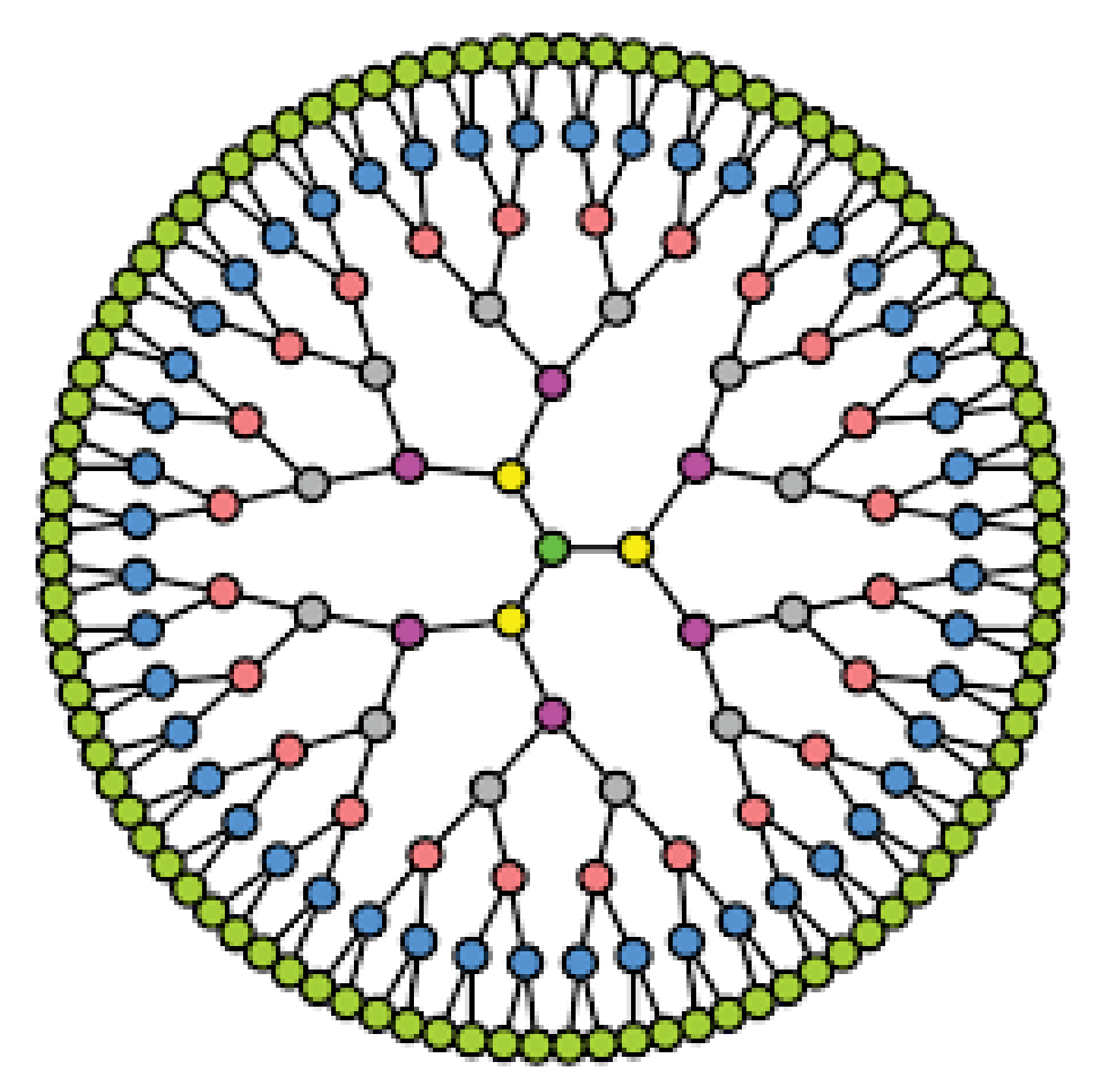
The reproduction number or $S^0,$ evaluates the pandemic’s intensity in epidemiology and is defined as the number of people who can become infected from a vulnerable population set. Figure 1 displays a pandemic tree for an epidemic with a $S^0$ (value of 4) epidemic.

The reproduction number of a pandemic, rounded to the closest integer, is $S^0$, and a pandemic tree is a full $S^0$-ary.

A rooted tree with no more than k offspring at each vertex is said to be k-ary. This vertex’s descendants include all of a node’s offspring. The height of a k-ary tree is defined as the greatest distance l from the leaf to the root vertex. Level 0 is referred to as the root vertex. According to induction, the offspring of vertices at level i are also at level $i+1.$ If every internal vertex on a k-ary tree has precisely k descendants, the tree is said to be complete. A pandemic tree is a full k-ary tree that has the epidemiological $S^0$ value of $k.$ rounded. This tree is represented by the letter ${\Omega }_l^k,$ where l indicates its height $k,l\ge 2$. 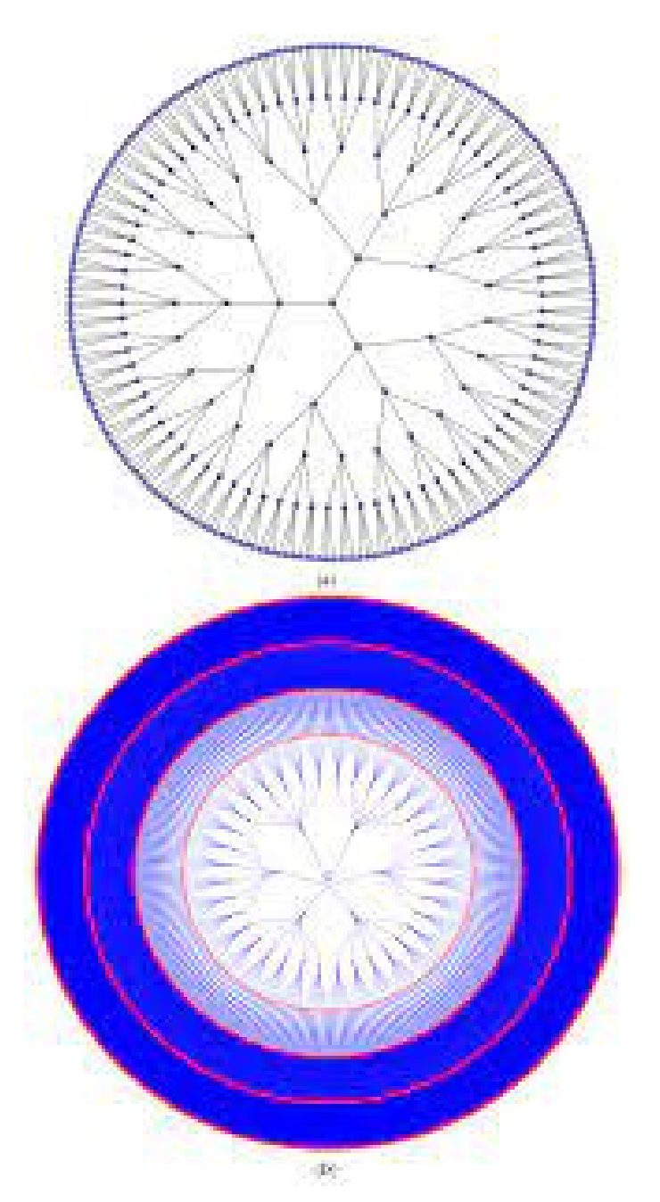Figure 2 depicts the pandemic tree levels 5 and 6.

Theorem 1. 

Let ${\Omega }_l^k$ stand for an epidemic tree with l levels and k reproductions. Then, $IS\left({\Omega }_l^k\right)=\frac{k^2(k+1)}{2k+1}+\frac{k^l(k+1)}{k+2}+{\displaystyle \sum _{i=1}^{l-2}}\frac{k^{l-i}(k+1)}{2}.$

Proof. 

For $i,0\le i\le 1,$ the number of vertices of ${\Omega }_l^k$ with level i is $k^i.$ Hence, we can easily calculate the total number of vertices and edges in ${\Omega }_l^k,$ that is, $\left|V\left({\Omega }_l^k\right)\right|=\frac{k^{l+1}-1}{k-1}$ and $\left|E\left({\Omega }_l^k\right)\right|=\frac{k^{l+1}-1}{k-1}-1.$ Now, we analyze the degree of any vertex x in ${\Omega }_l^k$ as follows;

(i)

If x is a leaf of ${\Omega }_l^k,$ then ${\lambda }_{{\Omega }_l^k}\left(x\right)=1.$

(ii)

If x is a root of ${\Omega }_l^k,$ then ${\lambda }_{{\Omega }_l^k}\left(x\right)=k.$

(iii)

If x is an internal vertex of ${\Omega }_l^k,$ then ${\lambda }_{{\Omega }_l^k}\left(x\right)=k+1.$

□

Let us consider the following edge partitions of a tree ${\Omega }_l^k$ based on its degrees of a edge. Let $P_{ij}$ be the set of all edges with degree of end vertices $i,j,$ that is, $P_{ij}=\{xy\in E\left({\Omega }_l^k\right)|{\lambda }_{{\Omega }_l^k}\left(x\right)=i,{\lambda }_{{\Omega }_l^k}\left(y\right)=j\}$ and let $p_{ij}$ be the number of edges in $P_{ij}.$ From the structure of ${\Omega }_l^k,$ it is clear that $p_{k+1,k}=k,$$p_{1,k+1}=k^l$ and $p_{k+1,k+1}={\displaystyle \sum _{i=1}^{l-2}}{k}^{l-i}.$ Thus,

$$\begin{array}{ccc}\hfill IS\left({\Omega }_l^k\right)& =& \sum _{xy\in E\left(T_l^k\right)}\frac{{\lambda }_{{\Omega }_l^k}\left(x\right){\lambda }_{{\Omega }_l^k}\left(y\right)}{{\lambda }_{{\Omega }_l^k}\left(x\right)+{\lambda }_{{\Omega }_l^k}\left(y\right)}\hfill \\ & =& p_{k+1,k}\left(\frac{{\lambda }_{{\Omega }_l^k}\left(x\right){\lambda }_{{\Omega }_l^k}\left(y\right)}{{\lambda }_{{\Omega }_l^k}\left(x\right)+{\lambda }_{{\Omega }_l^k}\left(y\right)}\right)+p_{1,k+1}\left(\frac{{\lambda }_{{\Omega }_l^k}\left(x\right){\lambda }_{{\Omega }_l^k}\left(y\right)}{{\lambda }_{{\Omega }_l^k}\left(x\right)+{\lambda }_{{\Omega }_l^k}\left(y\right)}\right)+p_{k+1,k+1}\left(\frac{{\lambda }_{{\Omega }_l^k}\left(x\right){\lambda }_{{\Omega }_l^k}\left(y\right)}{{\lambda }_{{\Omega }_l^k}\left(x\right)+{\lambda }_{{\Omega }_l^k}\left(y\right)}\right)\hfill \\ & =& k\left(\frac{(k+1)\times k}{(k+1)+k}\right)+k^l\left(\frac{(k+1)\times 1}{(k+1)+1}\right)+\sum _{i=1}^{l-2}{k}^{l-i}\times \left(\frac{(k+1)\times (k+1)}{(k+1)+(k+1)}\right)\hfill \\ & =& \frac{k^2(k+1)}{2k+1}+\frac{k^l(k+1)}{k+2}+\sum _{i=1}^{l-2}\frac{k^{l-i}(k+1)}{2}.\hfill \end{array}$$

3. Curtain Tree Network

Let $C_i$ represent a branch of a tree $\Omega$ created by connecting i pendant paths of length 2 to the vertex x in such a way that x has degree $i+1$ in $\Omega$. The curtain tree network, shown by $\Omega (r,C_k^s)$ in Figure 3, is created by joining s branches of $C_k$ to each vertex of path $P_r.$

Theorem 2. 

Let $r,s,k$ be three positive integers such that $r\ge 3,$$k\ge 2$ and $s\ge 1.$ Then, $IS(\Omega (r,C_k^s))=\frac{4krs(2k+6)}{3(k+3)}+s(k+1)\left(\frac{2(s+1)}{s+k+2}+\frac{s(r-2)}{s+k+1}\right)+\frac{2(s+1)(s+2)}{2s+3}+\frac{(r-3){(s+2)}^2}{2(s+2)}.$

Proof. 

We have $rs$ of branches $C_k$ based on the curtain tree network’s $\Omega (r,C_k^s)$ structure. We shall first mark all of the branches’ edges as follows:

(i)

$2k$ edges make up the branch of $C_k$, and k of those edges have two vertices: the first of degree one, and the second of degree two. Two vertices can be found on other k edges as well, the first of degree two and the second of degree $k+1.$

(ii)

The same is true for the $rs$ edges connecting the vertices of the route and the branches of $C_k$, $2s$ of which include two vertices, the first of degree $s+1$ and the second of degree $k+1.$ Two vertices are also present on the remaining $(r-2)s$ edges: one of degree $k+1$ and the other of degree $s+2.$

(iii)

Only the path’s edges are left at this point. This path has edges that are $r-1$. The first has a degree of $s+1$, and the second has a degree of $s+2.$ Two of them have two vertices. Additionally, there are two vertices with the same degree $s+2$ on the remaining $r-3$ edges.

□

Let $P_{ij}^{\prime }$ be the set of all edges with the degree of end vertices $i,j,$ that is, $P_{ij}^{\prime }=\{xy\in E(\Omega (r,C_k^s))|{\lambda }_{\Omega (r,C_k^s)}\left(x\right)=i,{\lambda }_{\Omega (r,C_k^s)}\left(y\right)=j\}$ and let $p_{ij}^{\prime }$ be the number of edges in $P_{ij}^{\prime }.$ From the structure of $\Omega (r,C_k^s),$ it is clear that $p_{1,2}^{\prime }=krs,$$p_{k+1,2}^{\prime }=krs,$$p_{k+1,s+1}^{\prime }=2s,$$p_{k+1,s}^{\prime }=s(r-2),$$p_{s+1,s+2}^{\prime }=2$ and $p_{s+2,s+2}^{\prime }=r-3.$ Thus

$$\begin{array}{ccc}\hfill IS(\Omega (r,C_k^s))& =& \sum _{xy\in E(\Omega (r,C_k^s))}\frac{{\lambda }_{\Omega (r,C_k^s)}\left(x\right){\lambda }_{\Omega (r,C_k^s)}\left(y\right)}{{\lambda }_{\Omega (r,C_k^s)}\left(x\right)+{\lambda }_{\Omega (r,C_k^s)}\left(y\right)}\hfill \\ & =& p_{1,2}^{\prime }(\frac{{\lambda }_{\Omega (r,C_k^s)}\left(x\right){\lambda }_{\Omega (r,C_k^s)}\left(y\right)}{{\lambda }_{\Omega (r,C_k^s)}\left(x\right)+{\lambda }_{\Omega (r,C_k^s)}\left(y\right)})+p_{k+1,2}^{\prime }(\frac{{\lambda }_{\Omega (r,C_k^s)}\left(x\right){\lambda }_{\Omega (r,C_k^s)}\left(y\right)}{{\lambda }_{\Omega (r,C_k^s)}\left(x\right)+{\lambda }_{\Omega (r,C_k^s)}\left(y\right)})\hfill \\ & & +p_{k+1,s+1}^{\prime }(\frac{{\lambda }_{\Omega (r,C_k^s)}\left(x\right){\lambda }_{\Omega (r,C_k^s)}\left(y\right)}{{\lambda }_{\Omega (r,C_k^s)}\left(x\right)+{\lambda }_{\Omega (r,C_k^s)}\left(y\right)})+p_{k+1,s}^{\prime }(\frac{{\lambda }_{\Omega (r,C_k^s)}\left(x\right){\lambda }_{\Omega (r,C_k^s)}\left(y\right)}{{\lambda }_{\Omega (r,C_k^s)}\left(x\right)+{\lambda }_{\Omega (r,C_k^s)}\left(y\right)})\hfill \\ & & +p_{s+1,s+2}^{\prime }(\frac{{\lambda }_{\Omega (r,C_k^s)}\left(x\right){\lambda }_{\Omega (r,C_k^s)}\left(y\right)}{{\lambda }_{\Omega (r,C_k^s)}\left(x\right)+{\lambda }_{\Omega (r,C_k^s)}\left(y\right)})+p_{s+2,s+2}^{\prime }(\frac{{\lambda }_{\Omega (r,C_k^s)}\left(x\right){\lambda }_{\Omega (r,C_k^s)}\left(y\right)}{{\lambda }_{\Omega (r,C_k^s)}\left(x\right)+{\lambda }_{\Omega (r,C_k^s)}\left(y\right)})\hfill \\ & =& krs\left(\frac{1\times 2}{1+2}\right)+krs\left(\frac{2\times (k+1)}{(k+1)+2}\right)+2s\left(\frac{(s+1)(k+1)}{(s+1)+(k+1)}\right)\hfill \\ & & +s(r-2)\left(\frac{s(k+1)}{s+(k+1)}\right)+2\left(\frac{(s+1)(s+2)}{(s+1)+(s+2)}\right)+r-3\left(\frac{(s+2)(s+2)}{(s+2)+(s+2)}\right)\hfill \\ & =& \frac{4krs(2k+6)}{3(k+3)}+s(k+1)\left(\frac{2(s+1)}{s+k+2}+\frac{s(r-2)}{s+k+1}\right)+\frac{2(s+1)(s+2)}{2s+3}+\frac{(r-3){(s+2)}^2}{2(s+2)}.\hfill \end{array}$$

4. Cayley Tree Network

A k-Cayley tree $CN(k,l)$ with levels l is a tree where all vertices have the same degree k except the leaves. Figure 4 depicts the Cayley tree’s structure, which has a degree of 3 and a level of 6.

Theorem 3. 

For a Cayley tree $CN(k,l),$ with $k,l\ge 3,$ we have $IS\left(CN(k,l)\right)=\frac{k(k{(k-1)}^l-k+1)}{2(k^2-3k+2)}+\frac{k^2{(k-1)}^l}{(k+1)}.$

Proof. 

Note that the number of vertices and edges in $CN(k,l)$ are, respectively, $\frac{k{(k-1)}^l-2}{k-2}$ and $\frac{k{(k-1)}^l-2}{k-2}-1.$ Let $P_{ij}^{\prime \prime }$ be the set of all edges of $CN(k,l)$ with a degree of end vertices $i,j$ and let $p_{ij}^{\prime \prime }$ be its cardinality. Then, by the structure of $CN(k,l),$ we have $p_{k,k}^{\prime \prime }=\frac{k{(k-1)}^l-k+1}{k^2-3k+2}$ and $p_{1,k}^{\prime \prime }=k{(k-1)}^{l-1}.$ Hence,

$$\begin{array}{ccc}\hfill IS\left(CN\right(k,l\left)\right)& =& \sum _{xy\in E\left(CN\right(k,l\left)\right)}\frac{{\lambda }_{CN(k,l)}\left(x\right){\lambda }_{CN(k,l)}\left(y\right)}{{\lambda }_{CN(k,l)}\left(x\right)+{\lambda }_{CN(k,l)}\left(y\right)}\hfill \\ & =& p_{k,k}^{\prime \prime }\frac{{\lambda }_{CN(k,l)}\left(x\right){\lambda }_{CN(k,l)}\left(y\right)}{{\lambda }_{CN(k,l)}\left(x\right)+{\lambda }_{CN(k,l)}\left(y\right)}+p_{1,k}^{\prime \prime }\frac{{\lambda }_{CN(k,l)}\left(x\right){\lambda }_{C(k,l)}\left(y\right)}{{\lambda }_{C(k,l)}\left(x\right)+{\mu }_{CN(k,l)}\left(y\right)}\hfill \\ & =& \frac{k{(k-1)}^l-k+1}{k^2-3k+2}\times \left(\frac{k\times k}{k+k}\right)+k{(k-1)}^{l-1}\times \left(\frac{k\times 1}{k+1}\right)\hfill \\ & =& \frac{k(k{(k-1)}^l-k+1)}{2(k^2-3k+2)}+\frac{k^2{(k-1)}^l}{(k+1)}.\hfill \end{array}$$

□

5. Christmas Tree Network

If a graph can be created from a Meyniel graph by eliminating every edge between any two nodes, it is said to be slim graph. A tree, also known as a linked acyclic undirected graph, is an undirected graph in graph theory in which any two vertices are connected by precisely one route. Thus, we can gain a slim tree in graph theory. For $s\ge 2,$ a Christmas tree $CTN\left(s\right)$ is composed of an $s^{th}$ slim tree $ST\left(s\right)=(V_1,E_1,u_1,l_1,r_1)$ and an ${(s+1)}^{th}$ slim tree $ST(s+1)=(V_2,E_2,u_2,l_2,r_2)$ together with the edges $u_1{u}_2,$$l_1{r}_2$ and $l_2{r}_1,$ where $ST\left(s\right)=(V,E,u,l,r),$ with V as the node set, E as the edge set, $u\in V$ as the root node, $l\in V$ as the left node, and $r\in V$ as the right node defined below:

$\left(i\right)$$ST\left(2\right)$ is the complete graph $K_3$ with its nodes labeled with $u,$l and $r.$

$\left(ii\right)$ The $s^{th}$ slim tree $ST\left(s\right),$ with $s\ge 3$ is composed of a root node u and two disjoint copies of ${(s-1)}^{th}$ slim trees as the left subtree and right subtree, denoted by $S{T}^l(s-1)=(V_1,E_1,u_1,l_1,r_1)$ and $S{T}^r(s-1)=(V_2,E_2,u_2,l_2,r_2),$ respectively, and $ST\left(s\right)=(V,E,u,l,r)$ is given by $V=V_1\cup V_2\cup \left\{u\right\},$$E=E_1\cup E_2\cup \{(u,u_1),(u,u_2),(r_1,l_2)\},$$l=l_1,r=r_2.$ For illustration, the Christmas tree $CT\left(3\right)$ is shown in Figure 5.

Theorem 4. 

For a Christmas tree $CTN\left(s\right),$$IS\left(CTN\left(s\right)\right)=(9\times 2^s-6)\times \frac{3}{4}$.

Proof. 

The number of vertices and edges of $CTN\left(s\right)$ are $(3\times 2^s)-2$ and $\frac{9\times 2^s-6}{2},$ respectively. As $CTN\left(s\right)$ is a 3-regular, $E_{3,3}=\{xy\in E\left(CTN\left(s\right)\right)|{\lambda }_{CTN\left(s\right)}\left(x\right)=3and{\lambda }_{CTN\left(s\right)}\left(y\right)=3\}$ is a only edge partition of $CTN\left(s\right)$ and its number of edges is $\frac{9\times 2^s-6}{2}.$ Hence,

$$\begin{array}{ccc}\hfill IS\left(CTN\right(s\left)\right)& =& \sum _{xy\in E\left(CTN\right(s\left)\right)}\frac{{\lambda }_{CTN\left(s\right)}\left(x\right){\lambda }_{CTN\left(s\right)}\left(y\right)}{{\lambda }_{CTN\left(s\right)}\left(x\right)+{\lambda }_{CTN\left(s\right)}\left(y\right)}\hfill \\ & =& \left|E_{3,3}\right|\left(\frac{3\times 3}{3+3}\right)=\frac{(9\times 2^s-6)}{2}\times \frac{9}{6}=(9\times 2^s-6)\times \frac{3}{4}.\hfill \end{array}$$

□

6. Corona Product of Graphs

Graph operations facilitate decomposition of a graph $\Omega$ into two or more isomorphic subgraphs. The corona product ${\Omega }_1\oplus {\Omega }_2$ of two graphs ${\Omega }_1$ and ${\Omega }_2$ is defined as the graph obtained by taking a copy of ${\Omega }_1$ and $\left|V\left({\Omega }_1\right)\right|$ copies of ${\Omega }_2,$ and then joining the $i^{th}$ vertex of ${\Omega }_1$ with edges to every vertex in the $i^{th}$ copy of ${\Omega }_2.$ It easily shows that $\left|V({\Omega }_1\oplus {\Omega }_2)\right|=\left|V\left({\Omega }_1\right)\right|+\left|V\left({\Omega }_1\right)\right|\left|V\left({\Omega }_2\right)\right|$ and $\left|E({\Omega }_1\oplus {\Omega }_2)\right|=\left|E\left({\Omega }_1\right)\right|+\left|V\left({\Omega }_1\right)\right|\left|E\left({\Omega }_2\right)\right|+\left|V\left({\Omega }_1\right)\right|\left|V\left({\Omega }_2\right)\right|.$ Now, we obtain the value for $ISI$ of corona product of Christmas tree $CTN\left(S\right)$ and a path graph $P_n.$

Theorem 5. 

If $CTN\left(S\right)\oplus P_n$ is a tree with $s,n\ge 2,$ then $IS(CTN\left(S\right)\oplus P_n)=(3\times 2^s-2)\left(\frac{6n+22}{n+5}+\frac{3(n-2)(n+3)}{n+6}+\frac{9(n-1)}{4}\right).$

Proof. 

The number of vertices and edges of $CTN\left(S\right)\oplus P_n$ are $3\times 2^s-2+(3\times 2^s-2)n$ and $\frac{9\times 2^s-6}{2}+((3\times 2^s)-2)(2n-1),$ respectively. From the structure of the corona product of $CTN\left(S\right)$ and $P_n,$ we have the following five edge partitions based on degrees of vertices;

$P_{n+3,n+3}=\{xy\in E(CTN\left(S\right)\oplus P_n)|{\lambda }_{CTN\left(S\right)\oplus P_n}\left(x\right)=n+3and{\lambda }_{CTN\left(S\right)\oplus P_n}\left(y\right)=n+3\},$

$P_{n+3,2}=\{xy\in E(CTN\left(S\right)\oplus P_n)|{\lambda }_{CTN\left(S\right)\oplus P_n}\left(x\right)=n+3and{\lambda }_{CTN\left(S\right)\oplus P_n}\left(y\right)=2\},$

$P_{n+3,3}=\{xy\in E(CTN\left(S\right)\oplus P_n)|{\lambda }_{CTN\left(S\right)\oplus P_n}\left(x\right)=n+3and{\lambda }_{CTN\left(S\right)\oplus P_n}\left(y\right)=3\},$

$P_{2,3}=\{xy\in E(CTN\left(S\right)\oplus P_n)|{\lambda }_{CTN\left(S\right)\oplus P_n}\left(x\right)=2and{\lambda }_{CTN\left(S\right)\oplus P_n}\left(y\right)=3\},$ and

$P_{3,3}=\{xy\in E(CTN\left(S\right)\oplus P_n)|{\lambda }_{CTN\left(S\right)\oplus P_n}\left(x\right)=3and{\lambda }_{CTN\left(S\right)\oplus P_n}\left(y\right)=3\}.$□

One can observe that $p_{n+3,n+3}=\frac{9\times 2^s-6}{2},$$p_{n+3,2}=2(3\times 2^s-2),$ $p_{n+3,3}=(n-2)(3\times 2^s-2),$$p_{2,3}=2(3\times 2^s-2)$ and $p_{3,3}=(n-3)(3\times 2^s-2).$ Hence

$$\begin{array}{ccc}\hfill IS(CTN\left(S\right)\oplus P_n)& =& \sum _{xy\in E(CTN\left(S\right)\oplus P_n)}\frac{{\lambda }_{CTN\left(S\right)\oplus P_n}\left(x\right){\lambda }_{CTN\left(S\right)\oplus P_n}\left(y\right)}{{\lambda }_{CTN\left(S\right)\oplus P_n}\left(x\right)+{\lambda }_{CTN\left(S\right)\oplus P_n}\left(y\right)}\hfill \\ & =& \frac{9\times 2^s-6}{2}\left(\frac{(n+3)\times (n+3)}{(n+3)+(n+3)}\right)+2(3\times 2^s-2)\left(\frac{(n+3)\times 2}{(n+3)+2}\right)\hfill \\ & & +(n-2)(3\times 2^s-2)\left(\frac{(n+3)\times 3}{(n+3)+3}\right)+2(3\times 2^s-2)\left(\frac{2\times 2}{2+2}\right)+(n-3)(3\times 2^s-2)\left(\frac{3\times 3}{3+3}\right)\hfill \\ & =& \frac{3(3\times 2^s-2)}{2}\left(\frac{(n+3)}{2}\right)+2(3\times 2^s-2)\left(\frac{2(n+3)}{n+5}\right)\hfill \\ & & +(n-2)(3\times 2^s-2)\left(\frac{3(n+3)}{n+6)}\right)+2(3\times 2^s-2)+\frac{3(n-3)(3\times 2^s-2)}{2}\hfill \\ & =& (3\times 2^s-2)\left(\frac{6n+22}{n+5}+\frac{3(n-2)(n+3)}{n+6}+\frac{9(n-1)}{4}\right).\hfill \end{array}$$

Theorem 6. 

The IS invariant of the corona product of two paths is $IS(P_r\oplus P_s)=\frac{32(s+1)}{(s+3)}+\frac{24(s-2)(s+1)+16(r-2)(s+2)}{(s+4)}+\frac{2(s+1)+2(r-3)(s+2)+6r(s-3)}{2}+\frac{34r}{5}+\frac{4(s+1)(s+2)}{(2s+3)}+\frac{6(s+2)(s-2)(r-2)}{(s+5)}.$

Proof. 

One can observe that the number of vertices and edges of the graph $P_r\oplus P_s$ are, respectively, $r+rs$ and $2rs-1.$ Let $P_{ij}$ be the set of all edges with the degree of end vertices $i,j,$ that is, $P_{ij}=\{xy\in E(P_r\oplus P_s)|{\lambda }_{P_r\oplus P_s}\left(x\right)=i,{\lambda }_{P_r\oplus P_s}\left(y\right)=j\}.$ Let $p_{ij}$ be the number of edges in $P_{ij}.$ From the structure of $P_r\oplus P_s,$ it is clear that

$p_{s+1,2}=4,$$p_{s+1,3}=2(s-2),$$p_{s+1,s+1}=\left\{\begin{array}{c}0\mathrm{if}r>2\hfill \\ 1\mathrm{if}r=2\hfill \end{array}\right.,$$p_{s+2,s+2}=\left\{\begin{array}{c}0\mathrm{if}r=2\hfill \\ r-3\mathrm{if}r>2\hfill \end{array}\right.,$$p_{s+1,s+2}=\left\{\begin{array}{c}0\mathrm{if}r=2\hfill \\ 2\mathrm{if}r>2\hfill \end{array}\right.,$$p_{s+2,2}=\left\{\begin{array}{c}0\mathrm{if}r=2\hfill \\ 2(r-2)\mathrm{if}r>2\hfill \end{array}\right.,$$p_{s+2,3}=\left\{\begin{array}{c}0\mathrm{if}r=2\hfill \\ (r-2)(s-2)\mathrm{if}r>2\hfill \end{array}\right.,$$p_{2,2}=\left\{\begin{array}{c}r\mathrm{if}s=2\hfill \\ 0\mathrm{if}s>2\hfill \end{array}\right.,$$p_{2,3}=\left\{\begin{array}{c}0\mathrm{if}s=2\hfill \\ 2r\mathrm{if}s>2\hfill \end{array}\right.$ and $p_{3,3}=\left\{\begin{array}{c}0\mathrm{if}s=2\hfill \\ r(s-3)\mathrm{if}s>2\hfill \end{array}\right..$ □

• If $r=s=2,$ then

$$\begin{array}{ccc}\hfill IS(P_r\oplus P_s)& =& \sum _{xy\in E\left(G\right)}\frac{{\lambda }_{P_r\oplus P_s}\left(x\right){\lambda }_{P_r\oplus P_s}\left(y\right)}{{\lambda }_{P_r\oplus P_s}\left(x\right)+{\lambda }_{P_r\oplus P_s}\left(y\right)}\hfill \\ & =& 4\left(\frac{2(s+1)}{(s+1)+2}\right)+2(s-2)\left(\frac{3(s+1)}{(s+1)+3}\right)+\left(\frac{(s+1)(s+1)}{(s+1)+(s+1)}\right)\hfill \\ & & +2(r-2)\left(\frac{2(s+2)}{(s+2)+2}\right)+r\left(\frac{2\times 2}{2+2}\right)\hfill \\ & =& \frac{8(s+1)}{(s+3)}+\frac{6(s-2)(s+1)}{(s+4)}+\frac{(s+1)}{2}+\frac{4(s+2)(r-2)}{(s+4)}+r\hfill \\ & =& \left(\frac{8(s+1)}{(s+3)}\right)+\left(\frac{(s+1)}{2}\right)+r+\left(\frac{6(s-2)(s+1)+4(r-2)(s+2)}{(s+4)}\right).\hfill \end{array}$$

• If $r=2$ and $s>2,$ then

$$\begin{array}{ccc}\hfill IS(P_r\oplus P_s)& =& 4\left(\frac{2(s+1)}{(s+1)+2}\right)+2(s-2)\left(\frac{3(s+1)}{(s+1)+3}\right)+\left(\frac{(s+1)(s+1)}{(s+1)+(s+1)}\right)\hfill \\ & & +2(r-2)\left(\frac{2(s+2)}{(s+2)+2}\right)\hfill \\ & & +2r\left(\frac{3\times 2}{3+2}\right)+r(s-3)\left(\frac{3\times 3}{3+3}\right)\hfill \\ & =& \frac{8(s+1)}{(s+3)}+\frac{6(s-2)(s+1)}{(s+4)}+\frac{(s+1)}{2}+\frac{4(s+2)(r-2)}{(s+4)}\hfill \\ & & +\frac{12r}{5}+\frac{3r(m-3)}{2}.\hfill \end{array}$$

• If $r=s=2,$ then

$$\begin{array}{ccc}\hfill IS(P_r\oplus P_s)& =& 4\left(\frac{2(s+1)}{(s+1)+2}\right)+2(s-2)\left(\frac{3(s+1)}{(s+1)+3}\right)+2\left(\frac{(s+1)(s+2)}{(s+1)+(s+2)}\right)\hfill \\ & & +(r-3)\left(\frac{(s+2)(s+2)}{(s+2)+(s+2)}\right)+2(r-2)\left(\frac{2(s+2)}{(s+2)+2}\right)\hfill \\ & & +(r-2)(s-2)\left(\frac{3(s+2)}{(s+2)+3}\right)+r\left(\frac{2\times 2}{2+2}\right)\hfill \\ & =& \frac{8(s+1)}{(s+3)}+\frac{6(s-2)(s+1)}{(s+4)}+\frac{2(s+1)(s+2)}{(2s+3)}+\frac{(r-3)(s+2)}{2}\hfill \\ & & +\frac{4(r-2)(s+2)}{(s+4)}+\frac{3(r-2)(s-2)(s+2)}{(s+5)}+r.\hfill \end{array}$$

• If $r>2$ and $s>2,$ then

$$\begin{array}{ccc}\hfill IS(P_r\oplus P_s)& =& 4\left(\frac{2(s+1)}{(s+1)+2}\right)+2(s-2)\left(\frac{3(s+1)}{(s+1)+3}\right)+2\left(\frac{(s+1)(s+2)}{(s+1)+(s+2)}\right)\hfill \\ & & +(r-3)\left(\frac{(s+2)(s+2)}{(s+2)+(s+2)}\right)+2(r-2)\left(\frac{2(s+2)}{(s+2)+2}\right)+(r-2)(s-2)\left(\frac{3(s+2)}{(s+2)+3}\right)\hfill \\ & & +2r\left(\frac{3\times 2}{3+2}\right)+r(s-3)\left(\frac{3\times 3}{3+3}\right)\hfill \\ & =& \frac{8(s+1)}{(s+3)}+\frac{6(s-2)(s+1)}{(s+4)}+\frac{2(s+1)(s+2)}{(2s+3)}+\frac{(r-3)(s+2)}{2}\hfill \\ & & +\frac{4(r-2)(s+2)}{(s+4)}+\frac{3(r-2)(s-2)(s+2)}{(s+5)}+\frac{12r}{5}+\frac{3r(s-3)}{2}.\hfill \end{array}$$

Theorem 7. 

The IS invariant of the corona product of two cycles is $IS(C_r\oplus C_s)=\frac{r(s+2)+3rs}{2}+\frac{3rs(s+2)}{(s+5)}.$

Proof. 

Clearly, the number of vertices and edges of the graph $C_r\oplus C_s$ are, respectively, $r+rs$ and $r+2rs$ when $r,s>2.$ Let $P_{ij}$ be the set of all edges with the degree of end vertices $i,j,$ that is, $P_{ij}=\{xy\in E(C_r\oplus C_s)|d_{C_r\oplus C_s}\left(x\right)=i,d_{C_r\oplus C_s}\left(y\right)=j\}.$ Let $p_{ij}$ be the number of edges in $P_{ij}.$ From the structure of $C_r\oplus C_s,$ it is clear that $p_{s+2,s+2}=r,$$p_{s+2,3}=rs$ and $p_{3,3}=rs.$ Thus,

$$\begin{array}{ccc}\hfill IS(C_r\oplus C_s)& =& \sum _{xy\in E(C_r\oplus C_s)}\frac{{\lambda }_{C_r\oplus C_s}\left(x\right){\lambda }_{C_r\oplus C_s}\left(y\right)}{{\lambda }_{C_r\oplus C_s}\left(x\right)+{\lambda }_{C_r\oplus C_s}\left(y\right)}\hfill \\ & =& r\left(\frac{(s+2)(s+2)}{(s+2)+(s+2)}\right)+rs\left(\frac{3(s+2)}{(s+2)+3}\right)+rs\left(\frac{3\times 3}{3+3}\right)\hfill \\ & =& \frac{r{(s+2)}^2}{2(s+2)}+\frac{3rs(s+2)}{(s+5)}+\frac{3sr}{2}\hfill \\ & =& \frac{r(s+2)+3rs}{2}+\frac{3rs(s+2)}{(s+5)}.\hfill \end{array}$$

□

Theorem 8. 

The IS invariant of the corona product of a complete graph $K_r$ and a path graph $P_s$ is $IS(K_r\oplus P_s)=\frac{r(r-1)(r+s-1)}{2}+\frac{8r(r+s-1)}{(r+s+1)}+\frac{6r(s-2)(r+s-1)}{(r+s+2)}+\frac{3r(s-3)}{2}+\frac{17r}{5}.$

Proof. 

One can observe that the number of vertices and edges of the graph $K_r\oplus P_s$ are, respectively, $r+rs$ and $rs+r(s-1)+\frac{r(r-1)}{2}.$ Let $P_{ij}$ be the set of all edges with the degree of end vertices $i,j,$ that is, $P_{ij}=\{xy\in E(K_r\oplus P_s)|d_{K_r\oplus P_s}\left(x\right)=i,d_{K_r\oplus P_s}\left(y\right)=j\}.$ Let $p_{ij}$ be the number of edges in $P_{ij}.$ From the structure of $P_r\oplus P_s,$ it is clear that

$p_{r+s-1,r+s-1}=\frac{r(r-1)}{2},$$p_{r+s-1,2}=2r,$$p_{r+s-1,3}=r(s-2),$$p_{2,2}=\left\{\begin{array}{c}0\mathrm{if}s>2\hfill \\ r\mathrm{if}s=2\hfill \end{array}\right.,$

$p_{2,3}=\left\{\begin{array}{c}0\mathrm{if}s=2\hfill \\ 2r\mathrm{if}s>2\hfill \end{array}\right.$ and $p_{3,3}=\left\{\begin{array}{c}0\mathrm{if}s=2\hfill \\ r(s-3)\mathrm{if}s>2\hfill \end{array}\right..$ Hence

• If $r\ge 2$ and $s=2,$ then

$$\begin{array}{ccc}\hfill IS(K_r\oplus P_s)& =& \sum _{xy\in E(K_r\oplus P_s)}\frac{{\lambda }_{K_r\oplus P_s}\left(x\right){\lambda }_{K_r\oplus P_s}\left(y\right)}{{\lambda }_{K_r\oplus P_s}\left(x\right)+{\lambda }_{K_r\oplus P_s}\left(y\right)}\hfill \\ & =& \frac{r(r-1)}{2}\left(\frac{(r+s-1)(r+s-1)}{(r+s-1)+(r+s-1)}\right)+2r\left(\frac{2(r+s-1)}{(r+s-1)+2}\right)\hfill \\ & & +r(s-2)\left(\frac{3(r+s-1)}{(r+s-1)+3}\right)+r\left(\frac{2\times 2}{2+2}\right)\hfill \\ & =& \frac{r(r-1)(r+s-1)}{4}+\frac{4r(r+s-1)}{(r+s+1)}+\frac{3r(s-2)(r+s-1)}{(r+s+2)}+r.\hfill \end{array}$$

• If $r\ge 2$ and $s>2,$ then

$$\begin{array}{ccc}\hfill IS(K_r\oplus P_s)& =& \frac{r(r-1)}{2}\left(\frac{(r+s-1)(r+s-1)}{(r+s-1)+(r+s-1)}\right)+2r\left(\frac{2(r+s-1)}{(r+s-1)+2}\right)\hfill \\ & & +r(s-2)\left(\frac{3(r+s-1)}{(r+s-1)+3}\right)+2r\left(\frac{3\times 2}{3+2}\right)+r(s-3)\left(\frac{3\times 3}{3+3}\right)\hfill \\ & =& \frac{r(r-1)(r+s-1)}{4}+\frac{4r(r+s-1)}{r+s+1}+\frac{3r(s-2)(r+s-1)}{r+s+2}+\frac{12r}{5}+\frac{3r(s-3)}{2}.\hfill \end{array}$$

□

It is easy to see that ${\Omega }_1\oplus {\Omega }_2$ is not in general isomorphic to ${\Omega }_2\oplus {\Omega }_1.$ Thus, the following theorem gives the value for $ISI$ of $P_r\oplus K_s.$

Theorem 9. 

$IS(P_r\oplus K_s)=\frac{4r^2(r+1)}{2r+1}+\frac{2r^2(r+1)+2(r+1)+(s+2)(s-3)}{2}+\frac{2(r+1)(r+2)}{2r+3}+\frac{r^2(r+2)(s-2)}{2(r+1)}.$

Proof. 

One can observe that the number of vertices and edges of the graph $P_r\oplus K_s$ are, respectively, $r+rs$ and $rs+(s-1)+\frac{sr(r-1)}{2}.$ Let $P_{ij}$ be the set of all edges with the degree of end vertices $i,j,$ that is, $P_{ij}=\{xy\in E(P_r\oplus K_s)|d_{P_r\oplus K_s}\left(x\right)=i,d_{P_r\oplus K_s}\left(y\right)=j\}.$ Let $p_{ij}$ be the number of edges in $P_{ij}.$ From the structure of $P_r\oplus K_s,$ it is clear that

$p_{r,r}=\frac{sr(r-1)}{2},$$p_{r,r+1}=2r,$$p_{r+1,r+1}=\left\{\begin{array}{c}0\mathrm{if}s>2\hfill \\ 1\mathrm{if}s=2\hfill \end{array}\right.,$$p_{r+1,r+2}=\left\{\begin{array}{c}0\mathrm{if}s=2\hfill \\ 2\mathrm{if}s>2\hfill \end{array}\right.,$

$p_{r+2,r}=\left\{\begin{array}{c}0\mathrm{if}s=2\hfill \\ r(s-2)\mathrm{if}s>2\hfill \end{array}\right.$ and $p_{r+2,r+2}=\left\{\begin{array}{c}0\mathrm{if}s=2\hfill \\ (s-3)\mathrm{if}m>2\hfill \end{array}\right..$ Hence

• If $r\ge 2$ and $s=2,$ then

$$\begin{array}{ccc}\hfill IS(P_r\oplus K_s)& =& \sum _{xy\in E(P_r\oplus K_s)}\frac{{\lambda }_{P_r\oplus K_s}\left(x\right){\lambda }_{P_r\oplus K_s}\left(y\right)}{{\lambda }_{P_r\oplus K_s}\left(x\right)+{\lambda }_{P_r\oplus K_s}\left(y\right)}\hfill \\ & =& \frac{(r+1)(r+1)}{(r+1)+(r+1)}+\frac{sr(r-1)}{2}\left(\frac{r\times r}{r+r}\right)+2r\left(\frac{r(r+1)}{r+(r+1)}\right)\hfill \\ & =& (r+1)+\frac{r^2(r-1)}{2}+\frac{2r^2(r+1)}{2r+1}.\hfill \end{array}$$

• If $r\ge 2$ and $s=2,$ then

$$\begin{array}{ccc}\hfill IS(P_r\oplus K_s)& =& \frac{sr(r-1)}{2}\left(\frac{r\times r}{r+r}\right)+2r\left(\frac{r(r+1)}{r+(r+1)}\right)+2\left(\frac{(r+1)(r+2)}{(r+1)+(r+2)}\right)\hfill \\ & & +(s-3)\left(\frac{(r+2)(r+2)}{(r+2)+(r+2)}\right)+r(s-2)\left(\frac{r(r+2)}{r+(r+2)}\right)\hfill \\ & =& \frac{r^2(r-1)}{2}+\frac{2r^2(r+1)}{2r+1}+\frac{2(r+1)(r+2)}{2r+3}+\frac{(s-3)(r+2)}{2}+\frac{r^2(s-2)(r+2)}{2r+2}.\hfill \end{array}$$

□

Theorem 10. 

The value of $IS$ of the corona product of two complete graphs is $IS(K_r\oplus K_s)=\frac{s^2(s-1)}{2}+\frac{r{s}^2(r+s-1)}{r+2s-1}+\frac{r(r-1)(r+s-1)}{4}.$

Proof. 

One can observe that the number of vertices and edges of the graph $K_r\oplus K_s$ are, respectively, $r+rs$ and $rs+(s-1)+\frac{sr(r-1)}{2}.$ Let $P_{ij}$ be the set of all edges with degree of end vertices $i,j,$ that is, $P_{ij}=\{xy\in E(K_r\oplus K_s)|{\lambda }_{K_r\oplus K_s}\left(x\right)=i,{\lambda }_{K_r\oplus K_s}\left(y\right)=j\}.$ Let $p_{ij}$ be the number of edges in $P_{ij}.$ From the structure of $K_r\oplus K_s,$ it is clear that $p_{s,s}=\frac{rs(s-1)}{2},$$p_{s,r+s-1}=rs$ and $p_{r+s-1,r+s-1}=\frac{r(r-1)}{2}.$ Hence,

$$\begin{array}{ccc}\hfill IS(K_r\oplus K_s)& =& \sum _{xy\in E(K_r\oplus K_s)}\frac{{\lambda }_{K_r\oplus K_s}\left(x\right){\lambda }_{K_r\oplus K_s}\left(y\right)}{{\lambda }_{K_r\oplus K_s}\left(x\right)+{\lambda }_{K_r\oplus K_s}\left(y\right)}\hfill \\ & =& s(s-1)\frac{s.s}{s+s}+rs\left(\frac{s(r+s-1)}{s+(r+s-1)}\right)+\frac{r(r-1)}{2}\left(\frac{(r+s-1)(r+s-1)}{(r+s-1)+(r+s-1)}\right)\hfill \\ & =& \frac{s^2(s-1)}{2}+\frac{r{s}^2(r+s-1)}{r+2s-1}+\frac{r(r-1)(r+s-1)}{4}.\hfill \end{array}$$

□

Corona products occasionally appear in chemical literature as plerographs of the typical hydrogen-suppressed molecular graphs known as Kneographs. For example, for a path $P_s,$ the graph $K_2\oplus P_s$ is called the bottleneck graph of $P_s.$ Let $C_t$ be the cycle with t vertices and define the molecular graph $T_{r,3}=G_r(C_3,v_1)$, which is the corona product of $P_r$ and $K_2.$ The fan graph $F_{s+1}=K_1\oplus P_s.$ By using above theorems, we obtain the following:

(i)

$ISI(K_2\oplus P_s)=\frac{(s+1)(s+19)}{s+3}+\frac{12(s-2)(s+1)}{s+4}+\frac{15s-11}{5},$

(ii)

$ISI(K_1\oplus P_s)=\frac{8s}{s+2}+\frac{6s(s-2)}{s+3}+\frac{15s-11}{10}$ and

(iii)

$ISI(P_r\oplus K_2)=\frac{4r^2(r+1)}{2r+1}+\frac{2(r+1)(r+2)}{2r+3}+(r+1)(r^2+1)-2.$

7. Bicyclic Graphs

The generic formula for the $IS$ invariant of various bicyclic graphs is given in this section. To start, we have the following assumption related to the jellyfish graph ${\Omega }^{C_k}(r,s,t).$ A linked graph is said to be bicyclic if there are one more edges than vertices in the graph. The Jellyfish graph is created by connecting two cycles of length r and s by a path of length t, then adding branches of length $Ck$ to each vertex in the two cycles and path (except from the terminal vertices in the path where we add one of $Ck$), as illustrated in Figure 6.

Theorem 11. 

Let $r,s,k$ be positive integers such that $r\ge 3,$$k\ge 2$ and $s\ge 1.$ Then, $IS\left({\Omega }^{C_k}(r,s,t)\right)=2(n+m+r-3)\left(\frac{2k(k+1)}{k+3}+\frac{4(k+1)}{k+5}+\frac{2k}{3}\right)+2(n+m+r-1).$

Proof. 

We have $2(r+s+t-3)$ of branches $Ck$ based on the ${\Omega }^{C_k}(r,s,t)$ structure of the Jellyfish graph. We shall first mark all of the branches’ edges as follows:

(i)

$2k$ edges make up the branch of $Ck$, and k of those edges have two vertices: the first of degree one, and the second of degree two. Two vertices, the first of degree two and the second of degree $k+1,$ may be found on another k edge of them.

(ii)

Additionally, there are $2(r+s+t-3)$ edges connecting branches of $Ck$ that each contain two vertices, the first of degree 4 and the second of degree $k+1.$

(iii)

We also have $r+s+t-1$ edges with degree 4 vertices in them.

□

Let $Q_{ij}^{\prime }$ be the set of all edges with the degree of end vertices $i,j,$ that is, $Q_{ij}=\{xy\in E(\Omega (r,C_k^s))|{\lambda }_{{\Omega }^{C_k}(r,s,t)}\left(x\right)=i,{\lambda }_{{\Omega }^{C_k}(r,s,t)}\left(y\right)=j\}.$ Let $q_{ij}$ be the number of edges in $Q_{ij}.$ From the structure of ${\Omega }^{C_k}(r,s,t),$ it is clear that $q_{1,2}=2k(r+s+t-3),$$q_{k+1,2}=2k(r+s+t-3),$$q_{k+1,4}=2(r+s+t-3)$ and $q_{4,4}=r+s+t-1.$ Thus,

$$\begin{array}{ccc}\hfill IS\left({\Omega }^{C_k}(r,s,t)\right)& =& \sum _{xy\in E\left({\Omega }^{C_k}(r,s,t)\right)}\frac{{\lambda }_{{\Omega }^{C_k}(r,s,t)}\left(x\right){\lambda }_{{\Omega }^{C_k}(r,s,t)}\left(y\right)}{{\lambda }_{{\Omega }^{C_k}(r,s,t)}\left(x\right)+{\lambda }_{{\Omega }^{C_k}(r,s,t)}\left(y\right)}\hfill \\ & =& q_{1,2}\left(\frac{1\times 2}{1+2}\right)+q_{k+1,2}\left(\frac{(k+1)\times 2}{(k+1)+2}\right)+q_{4,k+1}\left(\frac{4\times (k+1)}{(k+1)+4}\right)+p_{4,4}\left(\frac{4\times 4}{4+4}\right)\hfill \\ & =& 2k(r+s+t-3)\left(\frac{2}{3}\right)+2k(r+s+t-3)\left(\frac{2(k+1)}{(k+3)}\right)\hfill \\ & & +2(r+s+t-3)\left(\frac{4(k+1)}{(k+5)}\right)+2(r+s+t-1)\hfill \\ & =& 2(r+s+t-3)\left(\frac{2k(k+1)}{k+3}+\frac{4(k+1)}{k+5}+\frac{2k}{3}\right)+2(r+s+t-1).\hfill \end{array}$$

In order to discover a generic formula for $IS$, we will now examine applications of the bicyclic graph in chemistry, such as polycyclic alkanes, as seen in Figure 7. In order to produce numerous rings, two or more cycloalkanes are linked together to form polycyclic alkanes, which are molecules. The carbons of cycloalkanes are organized in the shape of a ring, making them cyclic hydrocarbons. Additionally, saturated cycloalkanes have single bonds between all of the carbon atoms that make up the ring (no double or triple bonds).

Classes of alkanes with one hydrogen atom removed are referred to as the group of alkyl or branches of alkyl. Its main equation is $C_n{H}_{2n+1}.$ It will include the branches of alkyl if n is larger than or equal to 1. A novel kind of bicyclic chemical graph is created when two separate chemical compounds are joined as cycloalkanes by an alkyl branch.

The molecular graph for the bicyclic chemical graphs is given by the symbol $C_{n,m}^{R_i},$ where n, m and r are the number of carbon atoms. The IS invariant connected to bicyclic chemical networks $C_{n,m}^{R_i}$ is given by the following theorem.

Theorem 12. 

Let $n,m,r$ be a positive integer such that $n,m\ge 3,$$r\ge 1.$ Then $IS\left(C_{n,m}^{R_i}\right)=\frac{18(n+m+r-1)}{5}.$

Proof. 

There are two different kinds of edges in the bicyclic chemical graphs $C_{n,m}^{R_i}.$ In this graph, we will first mark each edge as follows:

(i)

In the first kind, there are two vertices with the same degree of four on each of $n+m+r-1$ edges.

(ii)

In the second kind, there are two vertices of degree one and degree four that are incident on edges with the value $2(n+m+r-1)$.

□

Let $Q_{ij}^{\prime }$ be the set of all edges with the degree of end vertices $i,j,$ that is, $Q_{ij}^{\prime }=\{xy\in E\left(C_{n,m}^{R_i}\right)|{\lambda }_{C_{n,m}^{R_i}}\left(x\right)=i,{\lambda }_{C_{n,m}^{R_i}}\left(y\right)=j\}.$ Let $q_{ij}^{\prime }$ be the number of edges in $Q_{ij}^{\prime }.$ From the structure of $C_{n,m}^{R_i},$ it is clear that $q_{4,4}^{\prime }=n+m+r-1$ and $q_{1,4}^{\prime }=2(n+m+r-1).$ Thus,

$$\begin{array}{ccc}\hfill IS\left(C_{n,m}^{R_i}\right)& =& \sum _{xy\in E\left(C_{n,m}^{R_i}\right)}\frac{{\lambda }_{C_{n,m}^{R_i}}\left(x\right){\lambda }_{C_{n,m}^{R_i}}\left(y\right)}{{\lambda }_{C_{n,m}^{R_i}}\left(x\right)+{\lambda }_{C_{n,m}^{R_i}}\left(y\right)}\hfill \\ & =& q_{4,4}^{\prime }\left(\frac{4\times 4}{4+4}\right)+q_{1,4}^{\prime }\left(\frac{1\times 4}{1+4}\right)\hfill \\ & =& \frac{18(n+m+r-1)}{5}.\hfill \end{array}$$

Let $C_{n,r,m}^{R_s}$ be a bicyclic graph connected to a certain class of chemical compound’s molecular graph. This class’s molecular structure is created by combining two distinct cycloalkanes of lengths n and m with an alkyl branch of length r. We create a new class of bicyclic chemical graphs and the molecular graph $C_{n,r,m}^{R_s}$ that represents them by adding branches of alkyl $Rs$ to each hydrogen atom.

Theorem 13. 

Let r and s be positive integers such that $r\ge 3$ and $s\ge 1.$ Then, $IS\left(C_{n,r,m}^{R_s}\right)=\frac{2(2s+1)}{5}\left(9(n+m+r)-10s+1\right).$

Proof. 

We have $2(n+m+r-1)$ branches in the bicyclic graph $CRs$ when we consider its structure. First, we shall designate each branch’s margin as follows:

(i)

The branch of $R_s$ has $3s$ edges, $2s+1$ of which have two vertices, the first of degree 1 and the second of degree 4. Two vertices of degree 4 are also present in the remaining $s-1$ edges.

(ii)

We also have branches of $Rs$ with vertices of two cycles and a connecting route, each with two vertices of the same degree 4, and $2(n+r+m-1)$ edges linking those branches.

(iii)

The connecting path for all of the edges in this instance has two vertices of the same degree 4. We also have $n+m+r+1$ of edges that formed two cycles.

□

Let $Q_{ij}^{\prime \prime }$ be the set of all edges with the degree of end vertices $i,j,$ that is, $Q_{ij}^{\prime \prime }=\{xy\in E\left(C_{n,r,m}^{R_s}\right)|{\lambda }_{C_{n,r,m}^{R_s}}\left(x\right)=i,{\lambda }_{C_{n,r,m}^{R_s}}\left(y\right)=j\}.$ Let $q_{ij}^{\prime \prime }$ be the number of edges in $Q_{ij}^{\prime \prime }.$ From the structure of $C_{n,m}^{R_i},$ it is clear that $q_{1,4}^{\prime \prime }=(4s+2)(n+m+r-1)$ and $q_{4,4}^{\prime \prime }=(2s+1)(n+m+r)-2s+1.$ Thus,

$$\begin{array}{ccc}\hfill IS\left(C_{n,r,m}^{R_s}\right)& =& \sum _{xy\in E\left(C_{n,r,m}^{R_s}\right)}\frac{{\lambda }_{C_{n,r,m}^{R_s}}\left(x\right){\lambda }_{C_{n,r,m}^{R_s}}\left(y\right)}{{\lambda }_{C_{n,r,m}^{R_s}}\left(x\right)+{\lambda }_{C_{n,r,m}^{R_s}}\left(y\right)}\hfill \\ & =& q_{1,4}^{\prime }\left(\frac{1\times 4}{1+4}\right)+q_{4,4}^{\prime }\left(\frac{4\times 4}{4+4}\right)\hfill \\ & =& \frac{8(2s+1)(n+m+r-1)}{5}+2(2s+1)(n+m+r)-4s+2\hfill \\ & =& \frac{2(2s+1)}{5}\left(9(n+m+r)-10s+1\right).\hfill \end{array}$$

8. Conclusions

To create quantitative structure–activity relationships (QSAR), quantitative structure–property relationships (QSPR), and quantitative structure–toxicity relationships, topological indices (TI) are often utilized as molecular descriptors (QSTR). We have demonstrated in the present study that the TIs created are crucial for assessing the network data present in pandemic trees. The graph theoretical methods described here can also help with a variety of predictions about the dynamics of the ongoing epidemic. Last but not least, we calculated the degree-based entropy of the pandemic trees and the associated networks. These results significantly increased our understanding of how serious the continuing COVID-19 pandemic scenario is.

References

1. Ghani, M.U.; Campena, F.J.H.; Ali, S.; Dehraj, S.; Cancan, M.; Alharbi, F.M.; Galal, A.M. Characterizations of Chemical Networks Entropies by K-Banhatii Topological Indices. Symmetry 2023, 15, 143. [Google Scholar] [CrossRef]
2. Ghani, M.U.; Campena, F.J.H.; Maqbool, M.K.; Liu, J.-B.; Dehraj, S.; Cancan, M.; Alharbi, F.M. Entropy Related to K-Banhatti Indices via Valency Based on the Presence of C 6 H 6 in Various Molecules. Molecules 2023, 28, 452. [Google Scholar] [CrossRef] [PubMed]
3. Tag El Din, E.S.M.; Sultan, F.; Ghani, M.U.; Liu, J.-B.; Dehraj, S.; Cancan, M.; Alharbi, F.M.; Alhushaybari, A. Some Novel Results Involving Prototypical Computation of Zagreb Polynomials and Indices for SiO 4 Embedded in a Chain of Silicates. Molecules 2022, 28, 201. [Google Scholar] [CrossRef]
4. Ghani, M.U.; Maqbool, M.K.; George, R.; Ofem, A.E.; Cancan, M. Entropies Via Various Molecular Descriptors of Layer Structure of H3BO3. Mathematics 2022, 10, 4831. [Google Scholar] [CrossRef]
5. Mahmood, M.K.; Ali, S. A novel labeling algorithm on several classes of graphs. Punjab Univ. J. Math. 2017, 49, 23–35. [Google Scholar]
6. Ali, S.; Mahmmod, M.K.; Falcón Ganfornina, R.M. A paradigmatic approach to investigate restricted hyper totient graphs. AIMS Math. 2021, 6, 3761–3771. [Google Scholar] [CrossRef]
7. Ali, S.; Mahmood, M.K. A paradigmatic approach to investigate restricted totient graphs and their indices. Comput. Sci. 2021, 16, 793–801. [Google Scholar]
8. Mateen, M.H.; Mahmood, M.K.; Ali, S.; Alam, M.A. On symmetry of complete graphs over quadratic and cubic residues. J. Chem. 2021, 2021, 1–9. [Google Scholar] [CrossRef]
9. Chartrand, G.; Lesniak, L. Graphs and Digraphs; CRS Press: Boca Raton, FL, USA, 2005. [Google Scholar]
10. Devillers, J.; Balaban, A.T. Topological Indices and Related Descriptors in QSAR and QSPR; CRS Press: Boca Raton, FL, USA, 2000. [Google Scholar]
11. Gutman, I. A property of the simple topological index. MATCH Commun. Math. Comput. Chem. 1990, 25, 131–140. [Google Scholar]
12. Wiener, H. Structural determination of paraffin boiling points. J. Am. Chem. Soc. 1947, 69, 17–20. [Google Scholar] [CrossRef] [PubMed]
13. Amin, S.; Virk, A.U.R.; Rehman, M.A.; Shah, N.A. Analysis of dendrimer generation by sombor indices. J. Chem. 2021, 2021, 9930645. [Google Scholar] [CrossRef]
14. Hameed, M.S.; Al-Sabri, E.H.A.; Ahmad, Z.; Ali, S.; Ghani, M.U. Some Results on Submodules Using (μ,ν,ω)-Single-Valued Neutrosophic Environment. Symmetry 2023, 15, 247. [Google Scholar] [CrossRef]
15. Milano Chemometrics & QSAR Research Group, Molecular Descriptors Dataset. Available online: http://www.moleculardescriptors.eu/dataset/dataset.htm (accessed on 18 April 2014).
16. Zhang, Y.-F.; Ghani, M.U.; Sultan, F.; Inc, M.; Cancan, M. Connecting SiO 4 in Silicate and Silicate Chain Networks to Compute Kulli Temperature Indices. Molecules 2022, 27, 7533. [Google Scholar] [CrossRef]
17. Ghani, M.U.; Sultan, F.; Tag El Din, E.S.M.; Khan, A.R.; Liu, J.-B.; Cancan, M. A Paradigmatic Approach to Find the Valency-Based K-Banhatti and Redefined Zagreb Entropy for Niobium Oxide and a Metal–Organic Framework. Molecules 2022, 27, 6975. [Google Scholar] [CrossRef]
18. Balaban, A.T. Highly discriminating distance based numerical descriptor. Chem. Phys. Lett. 1982, 89, 399–404. [Google Scholar] [CrossRef]
19. Gutman, I.; Trinajstić, N. Graph theory and molecular orbitals. Total π-electron energy of alternant hydrocarbons. Chem. Phys. Lett. 1972, 17, 535–538. [Google Scholar] [CrossRef]
20. Karelson, M. Molecular Descriptors in QSAR/QSPR; Wiley-Interscience: New York, NY, USA, 2000. [Google Scholar]
21. Randić, M. On characterization of molecular branching. J. Am. Chem. Soc. 1975, 97, 6609–6615. [Google Scholar] [CrossRef]
22. Falahati-Nezhad, F.; Azari, M.; Doslic, T. Sharp bounds on the inverse sum indeg invariant. Discrete Appl. Math. 2017, 217, 185–195. [Google Scholar] [CrossRef]
23. Chu, Y.-M.; Khan, A.R.; Ghani, M.U.; Ghaffar, A.; Inc, M. Computation of zagreb polynomials and zagreb indices for benzenoid triangular & hourglass system. Polycycl. Aromat. Compd. 2022, in press. [Google Scholar]
24. Alam, A.; Ghani, M.U.; Kamran, M.; Hameed, M.S.; Khan, R.H.; Baig, A.Q. Degree-Based Entropy for a Non-Kekulean Benzenoid Graph. J. Math. 2022, 2022, 2288207. [Google Scholar]
25. Falahati-Nezhad, N.; Azari, M. The inverse sum indeg invariant of some nanotubes. Stud. Ubb Chem. 2016, 61, 63–70. [Google Scholar]
26. Sedlar, J.; Stevanović, D.; Vasilyev, A. On the inverse sum indeg inde. Discrete Appl. Math. 2015, 184, 202–212. [Google Scholar] [CrossRef]
27. Todeschini, R.; Consonni, V. Handbook of Molecular Descriptors; Wiley-VCH: Weinheim, Germany, 2000. [Google Scholar]
28. Gutman, I.; Polansky, O.E. Mathematical Concepts in Organic Chemistry; Springer: Berlin, Germany, 1986. [Google Scholar]
29. Trinajstic, N. Chemical Graph Theory, 2nd ed.; CRC Press: Boca Raton, FL, USA, 1983. [Google Scholar]
30. Nagarajan, S.; kumar, P.M.; Pattabiraman, K. Inverse Sum Indeg Invariant of Some Graphs. Eur. J. Math. Appl. 2021, 1, 1–8. [Google Scholar]
Figure 1. A pandemic tree with an eqidemiological R 0 value of 3.
Mathematics 11 00960 g001
Figure 2. A 5-level pandemic tree Ω 5 3 and 6-level pandemic tree Ω 6 6 .
Mathematics 11 00960 g002
Figure 3. A 5-level pandemic tree Ω 5 3 and 6-level pandemic tree Ω 6 6 .
Mathematics 11 00960 g003
Figure 4. A 3-Cayley tree C N ( 3 , 6 ) with 6 levels.
Mathematics 11 00960 g004
Figure 5. A Christmas tree C T N ( 3 ) with 3 levels.
Mathematics 11 00960 g005
Figure 6. The graph Ω C k ( r , s , t ) .
Mathematics 11 00960 g006
Figure 7. Molecular graph of polycyclic alkane.
Mathematics 11 00960 g007
Disclaimer/Publisher’s Note: The statements, opinions and data contained in all publications are solely those of the individual author(s) and contributor(s) and not of MDPI and/or the editor(s). MDPI and/or the editor(s) disclaim responsibility for any injury to people or property resulting from any ideas, methods, instructions or products referred to in the content.