A Fuzzy-Based Fast Feature Selection Using Divide and Conquer Technique in Huge Dimension Dataset

Abstract

Feature selection is commonly employed for identifying the top n features that significantly contribute to the desired prediction, for example, to find the top 50 or 100 genes responsible for lung or kidney cancer out of 50,000 genes. Thus, it is a huge time- and resource-consuming practice. In this work, we propose a divide-and-conquer technique with fuzzy backward feature elimination (FBFE) that helps to find the important features quickly and accurately. To show the robustness of the proposed method, it is applied to eight different datasets taken from the NCBI database. We compare the proposed method with seven state-of-the-art feature selection methods and find that the proposed method can obtain fast and better classification accuracy. The proposed method will work for qualitative, quantitative, continuous, and discrete datasets. A web service is developed for researchers and academicians to select top n features.

1. Introduction

A feature is an individual measurable property of the process being observed. A machine learning algorithm predicts the value of the desired target variable using these features [1]. We are now in the era of big data, where huge amounts of high-dimensional data have become ubiquitous in various domains, such as social media, healthcare, bioinformatics, and online education. The rapid growth of data presents challenges for feature selection. The “curse of dimensionality” (CoD), a wealth of riches, presents itself in various forms [2]. Feature Selection (variable elimination) helps understand the data, reduce computation requirements, reduce the effect of dimensionality’s curse, and improve the predictor performance.

Let, $\rho$ = number of observed variables.

Initially, as the dimensionality $\rho$ rises, the space that the samples could occupy expands rapidly. Figure 1 shows the model performance with respect to number for features. If we consider the distance between the points as a measure of similarity, then we interpret the greater distance as a greater dissimilarity. As $\rho$ increases, the pairwise distance between two points decreases, the correlation among vectors increases, and the likelihood of a specific region of the space being empty and sparse, with no data, increases.

In other words, as the number of dimensions grows, the amount of data required for satisfactory results from any machine learning algorithm expands rapidly. The cause of this is that with more dimensions, the model needs a greater number of data points to represent all the possible combinations of features in order to be considered valid.

Hughes (1968) found in his study that the effectiveness of a classifier in predicting outcomes improves as the number of dimensions increases up to a point [3]. Beyond that point, the performance decreases. This phenomenon of diminishing returns in prediction accuracy as the number of dimensions grows is commonly referred to as the “curse of dimensionality” or the “Hughes phenomenon”.

This study shows the requirement of feature selection, especially for a huge dimension dataset. Existing feature selection methods suffice for small datasets but fail in huge dimension datasets due to high computational requirements. A feature selection method removes features by measuring the relevance of each feature with the target class or by measuring the correlation between features. If two features are highly correlated, then one of them is removed. Feature selection methods are different from dimension reduction methods, such as PCA [1,4]. This is because good features can be independent from the rest of the data [5].

The outcome of a feature selection attempt from a broad dataset depends on several factors, such as the underlying probability distributions (some issues could be simple to solve), the number of instances (sample size), the number of features (dimensionality), the selected method for feature selection (its ability to find optimal feature subsets, its resistance to overfitting, and the accuracy of evaluating the desired criterion), and the classifier recommended to the user, as noted in [6].

Kohavil et al. propose the wrappers method for feature subset selection, which is divided into two major categories: filter and wrapper methods [7]. Filter methods score features without testing them in prediction algorithms, while in wrapper methods, the feature selection criteria are as per the predictor’s performance. The embedded method [8] is another technique that includes a variable method as a part of the training process.

2. Feature Selection Methods

2.1. Filter Methods

Filter methods choose features based on a measure of performance, independent of the data modeling algorithm used. The algorithm uses those features that are selected from filter methods. Filter methods can evaluate individual features or entire feature subsets, ranking them based on performance. These methods can be applied to various problems in classification, clustering, and regression, according to [9]. These criteria are mutual information, correlation, f-score, and chi-square.

2.1.1. Mutual Information

This method evaluates the dependency between two variables to score each of them. To understand mutual information [10], we must start with an entropy of variables.

Let X = random variable with discrete values. Then, the entropy of X, H(X) can be defined as

$$H\left(X\right)=-\sum p\left(x\right)logp\left(x\right),xϵX$$

(1)

where p(x) is the probability density function of x.

Conditional entropy refers to the uncertainty reduction of a variable when another is known. Assuming that variable Y is given, the conditional entropy H(X|Y) of X with respect to Y is

$$H\left(X\right|Y)=-\sum \sum p(x,y\left)logp\right(x\left|y\right),xϵX,yϵY$$

(2)

Equation (2) indicates that observing the variable X reduces the uncertainty in Y. The decrease in uncertainty is expressed as

$$I(Y,X)=H\left(Y\right)-H\left(Y\right|X)$$

(3)

This gives the mutual information between X and Y. Mutual information between X and Y will be zero if they are independent; greater than zero, they are dependent.

2.1.2. Correlation

Correlation is a statistical measure expressed as a number that characterizes the magnitude and direction of the relationship between two or more variables. The most commonly used measure of dependence between two variables is the Pearson correlation coefficient [11], which can be defined as

$${\rho }_{(X,Y)}=corr(X,Y)=\frac{cov(X,Y)}{{\sigma }_X{\sigma }_Y}=\frac{E\left[(X-{\mu }_X)(Y-{\mu }_Y)\right]}{{\sigma }_X{\sigma }_Y},if{\sigma }_X{\sigma }_Y>0$$

(4)

The above equation calculates the correlation between X and Y. The $cov(X,Y)$ calculates the covariance. The correlation ranking detects the correlation between features and the target variable.

2.1.3. Chi-Squared

A chi-squared test (symbolically represented as ${\chi }^2$) is a data analysis based on observations of a random set of variables. The chi-squared method evaluates the association of two categorical variables. The importance of a feature increases if its chi score is high [12]. Chi-squared statistics can be defined as follows:

$${\chi }^2=\sum _{i=1}^m\sum _{j=1}^k\left(\frac{A_{ij}-E_{ij}}{E_{ij}}\right)$$

(5)

where, m is the number of intervals, k is the number of classes, $A_{ij}$ is the number of samples in the ith interval of the jth class, $R_i$ is the number of samples in the ith interval, $C_j$ is the number of samples in the jth class, N is the total number of samples, and is the expected frequency of $A_{ij}(E_{ij}=R_i\ast C_j/N)$.

2.2. Wrapper Method

Wrapper methods employ a specific learning algorithm to assess the accuracy performance of a potential feature subset, leading to improved solutions [13]. In wrapper methods, a model is trained using a subset of features. Based on the performance of the model on these features, features are either added or removed from the subset. Some popular wrapper methods include forward selection, backward elimination, exhaustive feature selection, recursive feature elimination, and recursive feature elimination with cross-validation. Forward selection methods start with zero features and add up features according to relevance. After this, the final set of selected features is returned. Elimination methods start with the set of all features and eliminate features in every iteration until the desired number of features is obtained.

However, as this method requires training of the model on every iteration, it has a high computational cost [14]. As the number of features grows, the space of feature subsets grows exponentially. This becomes critical when tens of thousands of features are considered, for example, in a genomics dataset. As a result, the wrapper approach is largely avoided.

2.3. Embedded Method

Embedded methods are a combination of filter and wrapper methods that are iterative in nature. They differ from other feature selection methods, as they involve the incorporation of feature selection as a part of the training process [8]. During each iteration of the model training process, embedded methods carefully extract features that contribute the most to the training. Unlike wrapper methods, the link between feature selection and classification algorithms is stronger in embedded methods, as they use classification algorithms that contain their own built-in ability to select features [15].

3. Related Work

Filter methods in feature selection can be divided into two categories: feature weighting and subset search algorithms. Feature weighting algorithms determine which features are most important by assigning scores to individual features and ranking them based on these scores. On the other hand, subset search algorithms evaluate the goodness of entire feature subsets and choose the best one according to a certain evaluation measure [16].

A study merged two feature selection/extraction algorithms, independent component analysis (ICA) and fuzzy backward feature elimination (FBFE), and applied them to five DNA microarray datasets [17].

In a study by Yasmin et al., a graph-based feature selection approach was presented for language identification using rough-set boundary regions [18]. A new system was proposed that leverages the rough set theory to enhance the accuracy of language identification by using roughness from the theory to construct a weighted graph.

Reimann et al. tackle real-world-sized vehicle routing problems through their research [19]. They evaluate both established benchmark instances and new, larger-scale vehicle routing problem instances. The authors show that their approach not only improves efficiency, but also increases the algorithm’s effectiveness, leading to a highly effective tool for resolving real-world-sized vehicle routing problems.

Song et al. introduce a fast clustering-based feature subset selection algorithm that is designed for high-dimensional data [20]. The FAST algorithm consists of two phases. In the first phase, graph-based methods are utilized to classify features into clusters. In the next stage, the most significant features that have a strong association with the target classes are chosen from each cluster to form a subset of features.

Zhao et al. developed a recursive divide-and-conquer approach for sparse principal component analysis [21]. The approach divides the complex problem of sparse PCA into simpler sub-problems with known solutions and then solves each sub-problem recursively, resulting in a highly efficient algorithm for sparse PCA.

In the field of improving classification accuracy, multiple techniques have been proposed that aim to assign a shared discriminative feature set to the local behavior of data in different parts of the feature space [22,23]. One such method is localized feature selection (LFS), introduced by Armanfard et al. in which a subset of features is selected to fit a specific group of samples [23].

The class label of a new sample is assigned based on its similarity to the representative sample of each region in the feature space. The similarity is calculated for the sample’s arbitrary query. Some feature selection methods rank features by using aggregated sample data, such as in the case of the approaches introduced by Tibshirani et al. and Chen et al. [24,25].

Some of the feature selection approaches that would be used for comparison with the proposed feature selection methods are discussed below:

3.1. Minimum Redundancy Maximal Relevance Criteria (mRMR)

In mRMR, the maximum dependency condition (mutual information) is transformed into an equivalent form for incremental feature selection at the first order. This is followed by the application of a two-stage feature selection algorithm which merges mRMR with feature selection techniques, such as the wrapper method, leading to a cost-effective feature selection process [26].

3.2. Least Angle Regression (LARS)

In “least angle regression (LARS)”, three key properties are established [27]. The LARS algorithm is a less aggressive version of traditional forward selection methods and can be modified in three ways:

• A slight adjustment to LARS implements LASSO and calculates all possible LASSO estimates for a given problem.
• Another variation of LARS efficiently executes forward stagewise linear regression.
• A rough estimate of the degrees of freedom of a LARS estimate is available, allowing for a calculated prediction error estimate based on C${}_p$. This enables a deliberate choice among the possible LARS estimates.

3.3. Hilbert–Schmidt Independence Criterion LASSO (HSIC-LASSO)

In HISC-LASSO, a kernelized LASSO is utilized to identify nonlinear relationships between inputs and outputs [28]. By selecting appropriate kernel functions, features that have a strong statistical relationship with the target can be identified using the Hilbert–Schmidt independence criterion, a kernel-based measure of independence. These selected features are not redundant, and the globally optimal solution can be efficiently calculated, making this method suitable for high-dimensional problems.

3.4. Conditional Covariance Minimization (CCM)

The CCM method utilizes kernel-based independence measures to identify a subset of covariates that possess the maximum predictiveness of the response [29]. It achieves feature selection through an optimization problem that involves the trace of the conditional covariance operator.

3.5. Binary Coyote Optimization Algorithm (BCOA)

The binary constrained optimization algorithm (BCOA) [29] is an extension of the constrained optimization algorithm (COA) [30]. It performs feature selection by evaluating the performance of a binary classification algorithm. This is achieved by using the hyperbolic transfer function as a wrapper model to determine the optimal features.

4. Proposed Method

The proposed feature selection method employs the divide-and-conquer technique. This approach is recognized for its recursive execution of the same algorithm at lower levels, and eventually concludes after a finite period of time, as detailed in studies by Rosler [31] and Smith [32].

The divide-and-conquer method has the advantage of being able to tackle large problems efficiently by breaking them down into smaller sub-problems that can be solved individually [19]. This approach enables us to apply feature selection methods on large datasets, even if they are not capable of handling a huge number of features. The process involves dividing the features into smaller sets and then applying the selection methods to these subsets, leading to efficient resolution of the problem.

The aim is to select the top n features from a huge set of features (F). We achieve this by first dividing F into various subsets and finding the top features of these subsets using a feature selection method (such as the filter method). These subsets are then ranked according to their importance, and a new set of features is selected from this sorted set of features. The new set of top-selected features is further divided into subsets, and the process is repeated until we find the top n features of F. Now the problem we face is that any feature selection method can only select a certain number of features in desired constant time due to its computational efficiency. This limits the usability of that particular feature selection method. However, we can overcome this problem by using the divide-and-conquer approach.

To obtain the set of subsets of features shown in Figure 2, we first decide the size of this set of subsets of features. All the subsets will be of equal size because some of the features will be left out; these features will initially not be included in these subsets but will be evaluated later in the next iteration. L represents this set of features. We remove L from G and divide the remaining features into smaller subsets. A total of X subsets is formed. Each of these subsets is denoted by G${}_i$, where i ranges from 0 to X.

Now we will apply a filter method for feature selection in these X subsets and score each of the features in these subsets [33]. The filter method used in this paper is based on mutual information. Information gain, also known as mutual information, evaluates the impact of a feature on the accuracy of predicting the target. The concept assumes that if two random variables are independent, the information gain would be zero.

The selection of fuzzy functions is based upon a fuzzy entropy measurement. Since fuzzy entropy may better differentiate model distribution, it is used to evaluate the separability of each characteristic. The membership function used here is the Gaussian function. The Gaussian function is also known as the normal distribution function; it is often used in probability and statistics. The Gaussian function is used to represent fuzzy sets where the degree of membership for a given value is defined by the curve’s height at that value. The mean parameter ($\mu$) determines the center of the curve, and the standard deviation parameter ($\sigma$) determines the curve’s width. The area under the Gaussian curve equals 1, meaning that the membership function is normalized.

Intuitively, the lower the fuzzy entropy of a characteristic, the higher the capacity for discernment of the characteristic. The Shannon probabilistic entropy may be defined as [34]

$$H_1\left(A\right)=-\sum _{j=1}^n({\mu }_A\left(x_j\right)log{\mu }_A\left(x_j\right)+(1-{\mu }_A\left(x_j\right))log(1-m{u}_A\left(x_j\right)))$$

(6)

where ${\mu }_A\left(x_j\right)$ are the fuzzy values. This fuzzy entropy measurement is considered a measurement of fuzziness and assesses the overall deviations from the standard series type, i.e., any crisp set $A_0$ lead to h ($A_0$) = 0. Note that the fuzzy set A with ${\mu }_A\left(x_j\right)=0.5$ acts as the maximum element in the defined order by H. Newer fuzzy entropy measures [35] may improve the performance.

Apply a filter method for every G${}_i$ and arrange the features in descending order of importance in that subset. The first feature of each subset will be the most important feature of that subset. Using this, we will arrange every subset G${}_i$ according to its importance, i.e., arrange the subsets G${}_i$ in descending order of importance of their first feature. All the features are now sorted in each subset G${}_i$, and all the subsets G${}_i$ are also sorted with respect to each other.

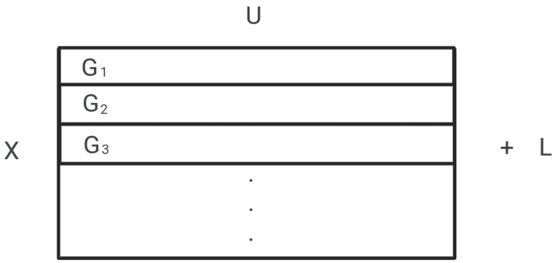
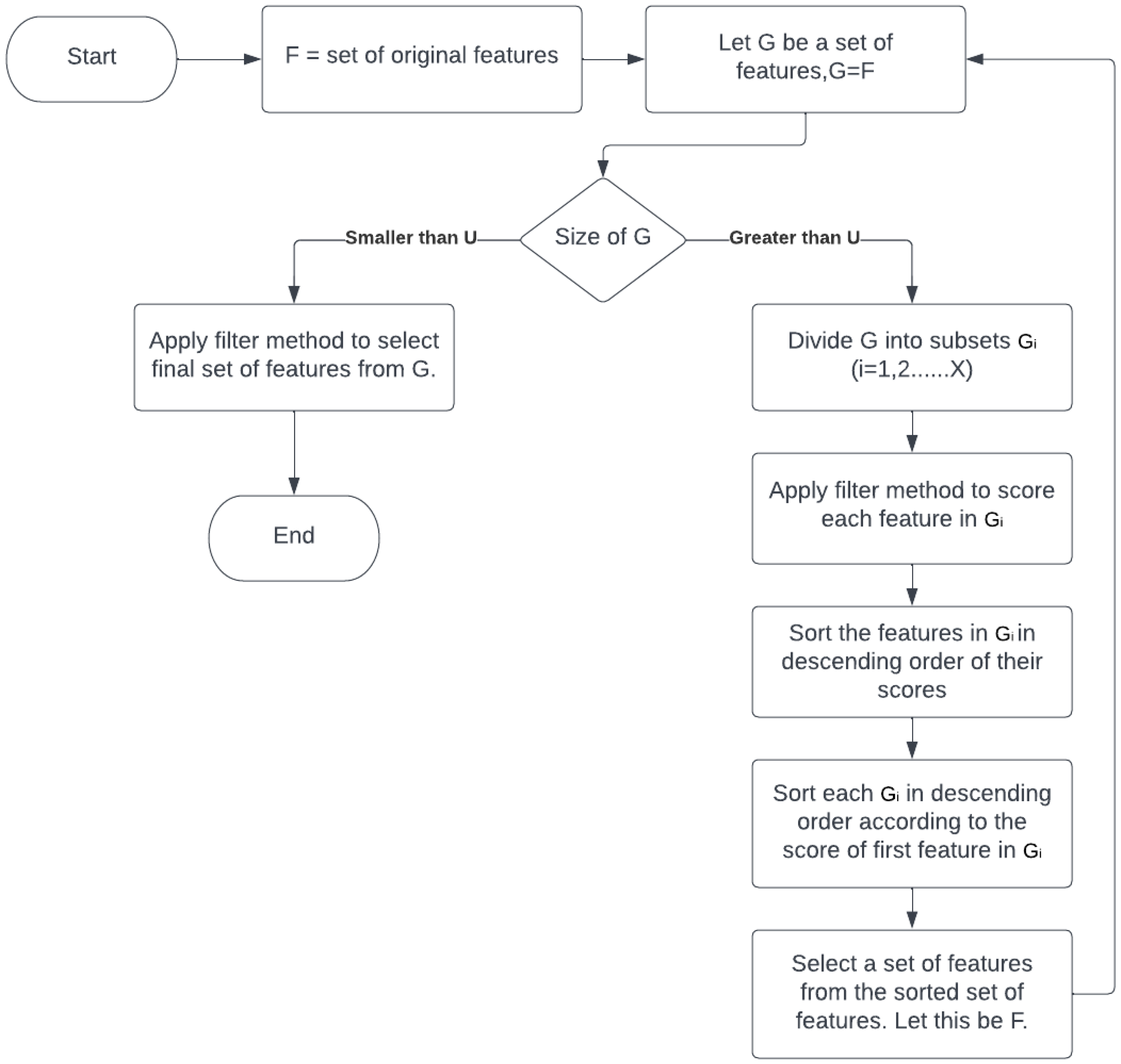
Let,         U = number of features; efficiently selected by feature selection method         from a group of features.         U will be the number of features in each subset, any feature selection         method would have to select a maximum of U features from each subset.         To divide the features into equal subsets, Let,         G = some set of features.         Initially, we will take the original set of features,         G = F. Let,         X = number of subsets,         L = set of features left after the division of G into equal subsets,         G${}_i$ = subset of G, i = 1, 2, 3, ⋯ , X; Then,         sizeof(G) = X × U + sizeof(L)         sizeof() represents the size of a set in single dimension. Given the values of G and U, we can find the value of X and L by,         X = $\lfloor \frac{sizeof\left(G\right)}{U}\rfloor$,         sizeof(L) = sizeof(G) - X × U

    The resulting matrix will have the most important features in the upper left corner, and the least important ones in the bottom right corner (according to the filter method’s score). We will split this matrix into two parts according to n (number of features required) and select the features in the upper part of the matrix to form a new set of features. G${}^{\prime }$ will now become the newly obtained set of features, and the process will be repeated until the top n features are selected.

The matrix is divided into two parts, i.e., G${}_i$ and G${}_{i-1}$. Each jth feature in G${}_i$ has more importance than $(j-1)$th. Similarly, for the feature in G${}_{i-1}$ (j = 1, 2, 3, ⋯, we do not know whether if the least important feature of G${}_i$ is more important than the most important feature of G${}_{i-1}$ or not. This is because the features of a subset are scored with respect to each other (i.e., scoring of features is done within the subset) and not with the features of another subset. Therefore the features that could potentially be the top n features are as follows.   

top n features of G${}_1$,        or top n-1 features of G${}_1$ + top feature of G${}_2$,        or top n-2 features of G${}_1$ + top 2 features of G${}_2$,        or top n-2 features of G${}_1$ + top feature of G${}_2$ + top feature of G${}_3$,        or top n-3 features of G${}_1$ + top 3 features of G${}_2$,        or top n-3 features of G${}_1$ + top 2 features of G${}_2$ + top feature of G${}_3$,        .        .        .   Keeping this in mind, the new subset of features(G) will be selected as,        G’ = {}, initially it will be an empty set,        For every subset of features G${}_i$, i = 1, 2, ⋯, X   Let,        $y=max(0,n-i+1)$,        G${}^{\prime }$ = G${}^{\prime }$ + top y feature of G${}_i$   The previous set of features G will be updated as,        G = G${}^{\prime }$ + L

    This process is repeated until the size of G is smaller than U. Now we apply the filter method to this final set of features to obtain the top n features of the original set of features, as the number of features to select (n) is smaller than U. The final number of features to be selected (i.e., n) should be smaller than U in order for the method to work.

The proposed feature selection method is shown in Figure 3. It was applied to each dataset, with 20, 30, 40, 50, and 60 features selected in each run. The selected features were then used to fit and train the modes, which included hyperparameter tuning. The time utilized by the proposed feature selection method was also recorded. The results were then compared to other feature selection methods.

The pseudocode of the proposed approach is explained in Algorithm 1.

Algorithm 1 Pseudocode of the proposed approach.

Require: - import required libraries - set upper limit of algorithm as 500 - set number of features to extract Function-1: Data(InputFile, numberOfFeatures) - define n as numberOfFeatures - define dataframe by reading input csv file - apply data pre-processing and split the data into train and test set Function-2: FeatureDivider(features, upper_limit) #This function will divide the given set of features into smaller set of features - Calculate the number of features that will be in each smaller set of features and divide the bigger set of features accordingly - Return the set of features and the features left out of the perfect sets Function-3: Feature_selector(featureSets, k, mod) #This function will select top k features from each subset and sort them #define the feature selection method as SelectKBest for i in every feature subset     - define curr_df as a feature subset     - sort the features in this subset - sort the subsets with themselves by compare in the best features of each subset for i in range(number of subsets)     for j in range(number of subsets)       - sort the subsets in ascending order according to their top feature - return the sorted subset of features as sorted_top_k Function-4: upper_matrix(sorted_top_k,left,left_features) #This function will select features from upper matrix and add left out features to int - Take out the features from upper matrix of sorted_top_k and append them into final_features - Append the left out features to final features - return final_features Main Function: main_fun(features,upper_limit,mod,k) #This function will remove undesired features in each iteration while number of features left > upper_limit     - left_features, feature_sets = feature_divider(features,upper_limit)     - sorted_top_k = feature_selector(feature_sets,k,mod)     - final_features = upper_matrix(sorted_top_k,left_features)     - features = final_features - run one final iteration which will select out desired number of features - selector = SelectKBest(mod,k=k) - selector_fit = selector.fit(x_train[features],y_train) - top_n_features = selector_fit.get_feature_names_out() - write these features into a text file Call the Main Function: # call the data function to execute the program - data(InputFile,20)

5. Experimental Results

The proposed method will be evaluated against seven leading feature selection techniques: mRMR [26], LARS [27], HSIC-LASSO [28], Fast-OSFS and Scalable [36], group-SAOLA [37], CCM [29], and BCOA [38]. The implementation of the proposed method has been made available in the form of code [39].

5.1. Dataset Used

Datasets were selected from the NCBI database [40]. NCBI is a provider of online biomedical and genomic information resources. The data found in the database is in soft file format and was transformed into CSV using an R program [41,42]. The program also cleaned the data, resulting in a reduction of features. The standardized data was then transformed using a standard scaler to enhance classifier performance.

Table 1. Description of the dataset used for the experiment.

Datasets	Samples	Original Features	Cleaned Features	Labels
GDS-1615	127	22,200	13,600	Three
GDS-2546	167	12,600	9500	Four
GDS-968	171	12,600	9100	Four
GDS-2545	171	12,600	9300	Four
GDS-3929	183	24,500	19,300	Two
GDS-1962	180	54,600	29,100	Four
GDS-531	173	12,600	9300	Two
GDS-2547	164	12,600	9300	Four

describe the dataset used in the experiment. A total of eight datasets were used for the experiment. The target features of these datasets were divided into two, three, and four classes, with approximately 192 samples in each dataset.

5.2. Classifier Used

The prediction models used are support vector machine (SVM) and random forest [43]. SVM is a classification algorithm that identifies the most influential cases, called support vectors, to form a decision boundary or hyperplane. Random forest, on the other hand, operates in four stages. It selects random samples from the dataset, builds a decision tree for each sample, obtains a prediction from each tree, and chooses the prediction with the most votes through a voting process.

The accuracy of the SVM [44] and random forest classifiers [45] can be improved by tuning their parameters. The experiment utilized grid search cross-validation to optimize the parameters of both classifiers. This approach trains the model using every combination of the specified parameters to find the optimal set, which results in increased accuracy.

The parameters of grid search CV for RF used in the experiment were:

’n estimators’: np.arange(50,200,30) ’max features’: np.arange(0.1, 1, 0.1) ’max depth’: [3, 5, 7, 9, 50, 100] ’max samples’: [0.3, 0.5, 0.8, 1]

where,

• n_estimators: The quantity of trees in the forest.
• max_features: The number of features considered to find the optimal split.
• max_depth: The highest level of the tree.
• max_samples: The number of samples taken from X to train each base estimator.
• np.arange: Produces evenly spaced values within a specified range.

The parameters of grid search CV for SVM used in the experiment were:

’c’ :[0.01, 1, 5, 10, 100] ’kernel’:(’linear’, ’poly’, ’rbf’, ’sigmoid’) ’gamma’ :(’scale’, ’auto’)

where,

• c: A regularization constant.
• kernel: Determines the type of kernel used in the algorithm.
• gamma: The kernel coefficient for ‘rbf’, ‘poly’, and ‘sigmoid’.

5.3. Result and Discussion

Table 2. Comparativeperformance of accuracy using random forest and support vector machine.

Datasets	Features Selected	RF	SVM	Time Taken (sec)
GDS1615	20	86.31	83.15	41.29
	30	88.42	86.31	41.2
	40	86.31	82.1	43.25
	50	87.36	88.42	43.87
	60	86.31	88.42	44.97
GDS968	20	76.52	77.41	35.9
	30	74.89	75.84	36.43
	40	73.35	74.21	37.26
	50	76.55	78.8	38.4
	60	78.06	81.26	38.82
GDS531	20	84.49	78.27	29.44
	30	85.29	79.84	22.32
	40	86.86	86.06	22.52
	50	86.09	83.75	22.9
	60	86.83	83.75	23.75
GDS2545	20	72.67	68.76	37.98
	30	78.09	71.04	38.49
	40	75.01	73.29	38.9
	50	70.15	69.53	39.84
	60	75.01	71.81	40.82
GDS1962	20	79.25	72.59	129.13
	30	78.51	73.33	116.72
	40	80	77.77	129.6
	50	79.25	76.29	130.06
	60	79.25	76.29	130.82
GDS3929	20	74.44	69.33	46.38
	30	72.93	69.41	45.37
	40	76.66	67.88	45.91
	50	74.36	67.91	46.37
	60	75.26	67.88	48.54
GDS2546	20	95.2	84	37.87
	30	95.2	85.59	38.01
	40	96	80.8	38.66
	50	95.2	82.4	36.88
	60	95.2	80	38.39
GDS2547	20	69.23	67.59	37.77
	30	70.03	68.39	38.2
	40	70.06	67.56	39.1
	50	70.83	68.39	38.07
	60	70.86	65.93	38.79

shows the quantity of selected features, the accuracy obtained, and the duration in seconds of each run of the proposed method for each dataset.

Table 3. Comparative performance of different feature selection techniques over five runs for each method. Format: accuracy (number of features).

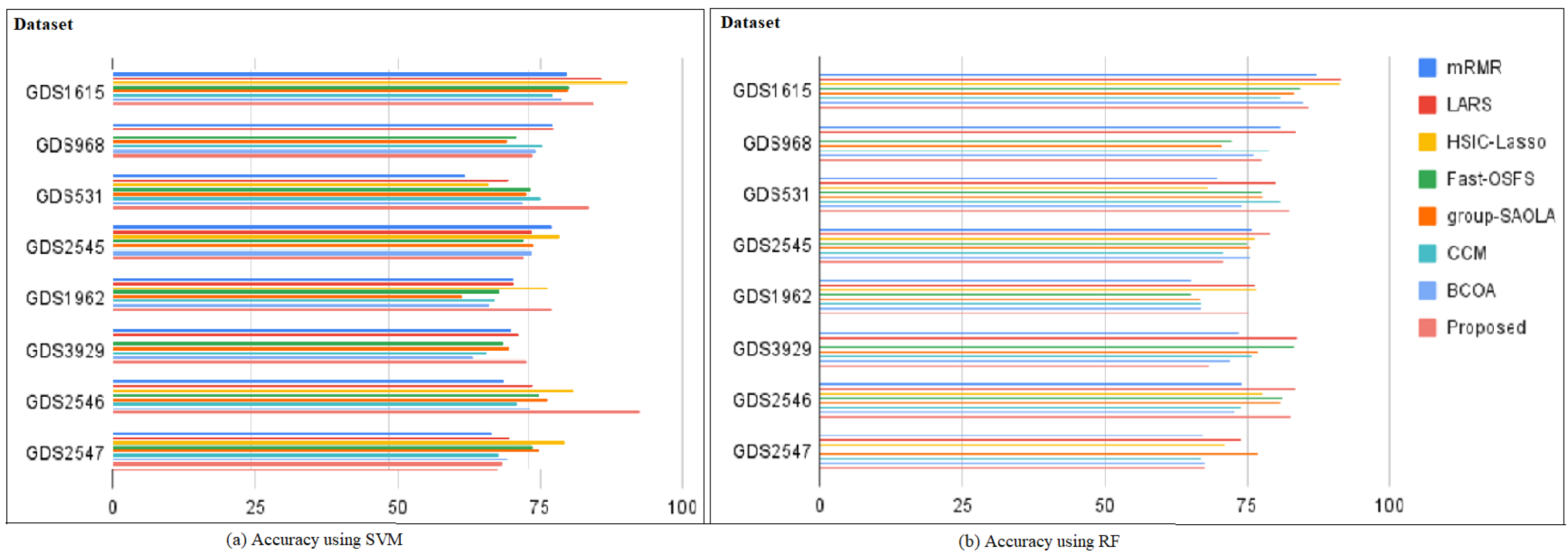
Classifier	Datasets	mRMR	LARS	HSIC	Fast	Group	CCM	BCOA	Proposed
				LASSO	OSFS	SAOLA	CCM	BCOA	Work
SVM	GDS1615	87.37(40)	91.67(26)	91.35(18)	84.31(17)	83.13(12)	80.82(29)	84.9(33)	88.42(50)
	GDS968	80.87(39)	83.73(38)	-	72.41(19)	70.53(14)	78.82(34)	76.19(32)	81.26(60)
	GDS531	69.78(30)	79.96(27)	67.93(4)	77.43(26)	77.7(11)	80.82(30)	74.17(32)	86.06(40)
	GDS2545	75.9(34)	79.02(33)	76.4(33)	74.95(18)	75.55(12)	70.82(30)	75.4(29)	73.29(40)
	GDS1962	65.12(39)	76.56(32)	76.81(31)	65.15(24)	66.59(10)	66.82(40)	66.89(35)	77.77(40)
	GDS3929	73.57(41)	83.78(41)	-	83.11(40)	76.97(21)	75.82(39)	72.12(41)	69.41(30)
	GDS2546	74.13(33)	83.51(32)	77.69(27)	81.25(26)	80.88(17)	73.82(35)	72.98(32)	85.59(30)
	GDS2547	67.31(39)	73.88(32)	71.16(12)	73.13(23)	76.85(24)	66.82(28)	67.35(26)	68.39(30)
RF	GDS1615	81.96(32)	88.24(20)	92.88(22)	82.34(15)	82.26(13)	79.55(31)	81.08(30)	88.42(30)
	GDS968	79.44(44)	79.77(42)	-	72.84(19)	71.28(18)	77.53(41)	76.42(40)	78.06(60)
	GDS531	63.69(23)	71.44(20)	67.82(4)	75.48(14)	74.67(16)	77.36(23)	73.92(21)	86.86(40)
	GDS2545	79.31(31)	75.81(33)	80.64(33)	74.16(14)	76.05(12)	74.82(34)	75.63(33)	78.09(30)
	GDS1962	72.37(29)	72.41(30)	78.45(42)	69.88(21)	63.28(13)	69.17(32)	67.95(30)	80(40)
	GDS3929	71.94(29)	73.44(28)	-	70.49(28)	71.56(15)	67.5(28)	65.13(24)	76.66(40)
	GDS2546	70.53(36)	75.86(34)	83.09(45)	77.04(25)	78.46(18)	72.9(36)	75.28(31)	96(40)
	GDS2547	68.44(22)	71.68(24)	81.67(32)	75.85(30)	77.1(20)	69.7(25)	71.28(24)	70.86(60)

presents the average number of selected features and average classification accuracy obtained over 10 separate runs using SVM and RF on the described datasets. The accuracy of the proposed method is based on the average of five runs, with the number of selected features set to 20, 30, 40, 50, and 60, respectively, and the parameter U fixed at 500 in each run.

Fuzzy backward feature elimination helps to identify the most relevant features in a dataset. By eliminating features that are less important or irrelevant, the algorithm can improve the performance of the model and make it more interpretable. Additionally, it can also help to identify potential sources of noise or bias in the dataset, which can improve the overall accuracy and generalizability of the model.

The proposed features selection method achieved better accuracy than the existing methods in the majority of the cases in a considerably smaller amount of time as compared to the existing methods. It also had considerably low computation requirements, which is beneficial, as this method can be used by anyone on low-performance machines, such as personal computers. This gain in efficiency might not be very observable in small datasets, but it drastically reduces the time required in feature selection in huge dimension datasets.

Figure 4 compares different feature selection techniques using a support vector machine and random forest on different datasets. The techniques compared include traditional methods, such as mutual information and correlation-based feature selection, as well as more recent methods, such as recursive feature elimination and LASSO. The results indicate that the proposed feature selection method surpasses all other techniques in terms of accuracy and computational efficiency. This is likely because the proposed method considers the interactions between features, whereas traditional methods focus solely on individual feature importance. The proposed method’s ability to select the most relevant features for the task at hand results in a more robust and accurate model.

The empty spaces in Table 3 mean that those specific feature selection methods do not run on the datasets. The accuracy achieved by the proposed method is better than other methods in most cases for SVM and random forest classifiers. The number of features selected was higher than in other methods. As the number of features selected was increased, the accuracy was increased in some cases but did not vary much, which shows that the method is rational.

This method does not require high computational power and can run on most machines. This was possible because of the divide-and-conquer approach, which reduced the complexity of the problem. The time taken by the proposed method was significantly less, keeping the required time under 1 m for five datasets, 30 s for one dataset, and about 2 m for one dataset.

6. Application of the Proposed Work

The proposed method, apart from genomic datasets, can be used in various areas, such as in healthcare datasets, where the number of features for a given individual can be massive (i.e., blood pressure, blood group, resting heart rate, height, weight, immune system status, surgery history, nutrition, and existing conditions), in financial datasets, where the number of features for a given stock can be quite large, and in ecological datasets.

Contour shape analysis is a demonstration of data analysis in infinite dimensions, specifically, analysis on the projective spaces of a Hilbert space. This method involves using high-dimensional approximations and operates within the framework of a Hilbert manifold.

The proposed method uses the divide-and-conquer technique with fuzzy backward feature elimination (FBFE) that helps to find the important features quickly and accurately. To show the robustness of the proposed method, it is applied to eight different datasets taken from the NCBI database. The only requirement is that the selection method scores each feature for the divide-and-conquer approach to work. This opens up a vast area of research where few feature selection methods can be used over this method.

7. Conclusions

This paper presents a feature selection method to select the top n important features from a huge dimensional dataset. The novelty of our method is that it can run on a huge set of features in less time and use less computational power. It uses a divide-and-conquer approach to select the top n important features from the datasets. The proposed method performed well compared to other state-of-the-art feature selection methods on the datasets. This method can be made more accurate by using other feature selection methods, such as wrapper and exhaustive feature selection methods, instead of filter methods.

In this paper, the focus was only on genomics datasets, as these are widely accepted, and only a few dimension reduction algorithms work well on these datasets. In future work, we aim to revise our feature selection method and use wrapper methods with this proposed method.

References

- Chandrashekar, G.; Sahin, F. A survey on feature selection methods. Comput. Electr. Eng. 2014, 40, 16–28. [Google Scholar] [CrossRef]
- Altman, N.; Krzywinski, M. The curse(s) of dimensionality. Nat. Methods 2018, 15, 399–400. [Google Scholar] [CrossRef] [PubMed]
- Hughes, G. On the mean accuracy of statistical pattern recognizers. IEEE Trans. Inf. Theory 1968, 14, 55–63. [Google Scholar] [CrossRef]
- Baştanlar, Y.; Özuysal, M. Introduction to machine learning. In miRNomics: MicroRNA Biology and Computational Analysis; Humana Press: Totowa, NJ, USA, 2014; pp. 105–128. [Google Scholar]
- Law, M.H.; Figueiredo, M.A.; Jain, A.K. Simultaneous feature selection and clustering using mixture models. IEEE Trans. Pattern Anal. Mach. Intell. 2004, 26, 1154–1166. [Google Scholar] [CrossRef] [PubMed]
- Kuncheva, L.I.; Matthews, C.E.; Arnaiz-González, Á.; Rodríguez, J.J. Feature selection from high-dimensional data with very low sample size: A cautionary tale. arXiv 2020, arXiv:2008.12025. [Google Scholar]
- Kohavi, R.; John, G.H. Wrappers for feature subset selection. Artif. Intell. 1997, 97, 273–324. [Google Scholar] [CrossRef]
- Blum, A.L.; Langley, P. Selection of relevant features and examples in machine learning. Artif. Intell. 1997, 97, 245–271. [Google Scholar] [CrossRef]
- Jović, A.; Brkić, K.; Bogunović, N. A review of feature selection methods with applications. In Proceedings of the 2015 38th International Convention on Information and Communication Technology, Electronics and Microelectronics (MIPRO), Opatija, Croatia, 25–29 May 2015; pp. 1200–1205. [Google Scholar]
- Liu, H.; Sun, J.; Liu, L.; Zhang, H. Feature selection with dynamic mutual information. Pattern Recognit. 2009, 42, 1330–1339. [Google Scholar] [CrossRef]
- Battiti, R. Using mutual information for selecting features in supervised neural net learning. IEEE Trans. Neural Netw. 1994, 5, 537–550. [Google Scholar] [CrossRef]
- Wah, Y.B.; Ibrahim, N.; Hamid, H.A.; Abdul-Rahman, S.; Fong, S. Feature Selection Methods: Case of Filter and Wrapper Approaches for Maximising Classification Accuracy. Pertanika J. Sci. Technol. 2018, 26, 329–340. [Google Scholar]
- El Aboudi, N.; Benhlima, L. Review on wrapper feature selection approaches. In Proceedings of the 2016 International Conference on Engineering & MIS (ICEMIS), Agadir, Morocco, 22–24 September 2016; pp. 1–5. [Google Scholar]
- Bolón-Canedo, V.; Sánchez-Marono, N.; Alonso-Betanzos, A.; Benítez, J.M.; Herrera, F. A review of microarray datasets and applied feature selection methods. Inf. Sci. 2014, 282, 111–135. [Google Scholar] [CrossRef]
- Liu, H.; Zhou, M.; Liu, Q. An embedded feature selection method for imbalanced data classification. IEEE/CAA J. Autom. Sin. 2019, 6, 703–715. [Google Scholar] [CrossRef]
- Liu, H.; Motoda, H. Feature Extraction, Construction and Selection: A Data Mining Perspective; Springer Science & Business Media: Berlin/Heidelberg, Germany, 1998; Volume 453. [Google Scholar]
- Aziz, R.; Verma, C.; Srivastava, N. A fuzzy based feature selection from independent component subspace for machine learning classification of microarray data. Genom. Data 2016, 8, 4–15. [Google Scholar] [CrossRef]
- Yasmin, G.; Das, A.K.; Nayak, J.; Pelusi, D.; Ding, W. Graph based feature selection investigating boundary region of rough set for language identification. Expert Syst. Appl. 2020, 158, 113575. [Google Scholar] [CrossRef]
- Reimann, M.; Doerner, K.; Hartl, R.F. D-ants: Savings based ants divide and conquer the vehicle routing problem. Comput. Oper. Res. 2004, 31, 563–591. [Google Scholar] [CrossRef]
- Song, Q.; Ni, J.; Wang, G. A fast clustering-based feature subset selection algorithm for high-dimensional data. IEEE Trans. Knowl. Data Eng. 2011, 25, 1–14. [Google Scholar] [CrossRef]
- Zhao, Q.; Meng, D.; Xu, Z. A recursive divide-and-conquer approach for sparse principal component analysis. arXiv 2012, arXiv:1211.7219. [Google Scholar]
- Sun, Y.; Todorovic, S.; Goodison, S. Local-learning-based feature selection for high-dimensional data analysis. IEEE Trans. Pattern Anal. Mach. Intell. 2009, 32, 1610–1626. [Google Scholar]
- Armanfard, N.; Reilly, J.P.; Komeili, M. Local feature selection for data classification. IEEE Trans. Pattern Anal. Mach. Intell. 2015, 38, 1217–1227. [Google Scholar] [CrossRef]
- Tibshirani, R. Regression shrinkage and selection via the lasso. J. R. Stat. Soc. Ser. (Methodol.) 1996, 58, 267–288. [Google Scholar] [CrossRef]
- Chen, X.; Yuan, G.; Nie, F.; Huang, J.Z. Semi-supervised Feature Selection via Rescaled Linear Regression. In Proceedings of the IJCAI, Melbourne, Australia, 19–25 August 2017; Volume 2017, pp. 1525–1531. [Google Scholar]
- Peng, H.; Long, F.; Ding, C. Feature selection based on mutual information criteria of max-dependency, max-relevance, and min-redundancy. IEEE Trans. Pattern Anal. Mach. Intell. 2005, 27, 1226–1238. [Google Scholar] [CrossRef] [PubMed]
- Efron, B.; Hastie, T.; Johnstone, I.; Tibshirani, R. Least angle regression. Ann. Stat. 2004, 32, 407–499. [Google Scholar] [CrossRef]
- Yamada, M.; Jitkrittum, W.; Sigal, L.; Xing, E.P.; Sugiyama, M. High-dimensional feature selection by feature-wise kernelized lasso. Neural Comput. 2014, 26, 185–207. [Google Scholar] [CrossRef] [PubMed]
- Chen, J.; Stern, M.; Wainwright, M.J.; Jordan, M.I. Kernel feature selection via conditional covariance minimization. Adv. Neural Inf. Process. Syst. 2017, 30, 6949–6958. [Google Scholar]
- Pierezan, J.; Coelho, L.D.S. Coyote optimization algorithm: A new metaheuristic for global optimization problems. In Proceedings of the 2018 IEEE congress on evolutionary computation (CEC), Brisbane, Australia, 10–15 June 2018; pp. 1–8. [Google Scholar]
- Rösler, U. On the analysis of stochastic divide and conquer algorithms. Algorithmica 2001, 29, 238–261. [Google Scholar] [CrossRef]
- Smith, D.R. The design of divide and conquer algorithms. Sci. Comput. Program. 1985, 5, 37–58. [Google Scholar] [CrossRef]
- Guyon, I.; Gunn, S.; Nikravesh, M. Feature Extraction: Studies in Fuzziness and Soft Computing; Springer Science & Business Media: Berlin/Heidelberg, Germany, 2006. [Google Scholar]
- Luukka, P. Feature selection using fuzzy entropy measures with similarity classifier. Expert Syst. Appl. 2011, 38, 4600–4607. [Google Scholar] [CrossRef]
- Parkash, O.; Gandhi, C. Applications of trigonometric measures of fuzzy entropy to geometry. Int. J. Math. Comput. Sci 2010, 6, 76–79. [Google Scholar]
- Yu, L.; Liu, H. Feature selection for high-dimensional data: A fast correlation-based filter solution. In Proceedings of the 20th International Conference on Machine Learning (ICML-03), Washington, DC, USA, 21–24 August 2003; pp. 856–863. [Google Scholar]
- Yu, K.; Ding, W.; Wu, X. LOFS: A library of online streaming feature selection. Knowl.-Based Syst. 2016, 113, 1–3. [Google Scholar] [CrossRef]
- De Souza, R.C.T.; de Macedo, C.A.; dos Santos Coelho, L.; Pierezan, J.; Mariani, V.C. Binary coyote optimization algorithm for feature selection. Pattern Recognit. 2020, 107, 107470. [Google Scholar] [CrossRef]
- Available online: https://github.com/git-arihant/feature-importance (accessed on 25 December 2022).
- Available online: https://www.ncbi.nlm.nih.gov/ (accessed on 25 December 2022).
- Available online: https://github.com/jranaraki/NCBIdataPrep (accessed on 25 December 2022).
- Afshar, M.; Usefi, H. High-dimensional feature selection for genomic datasets. Knowl.-Based Syst. 2020, 206, 106370. [Google Scholar] [CrossRef]
- Sheykhmousa, M.; Mahdianpari, M.; Ghanbari, H.; Mohammadimanesh, F.; Ghamisi, P.; Homayouni, S. Support vector machine versus random forest for remote sensing image classification: A meta-analysis and systematic review. IEEE J. Sel. Top. Appl. Earth Obs. Remote. Sens. 2020, 13, 6308–6325. [Google Scholar] [CrossRef]
- Yuanyuan, S.; Yongming, W.; Lili, G.; Zhongsong, M.; Shan, J. The comparison of optimizing SVM by GA and grid search. In Proceedings of the 2017 13th IEEE International Conference on Electronic Measurement & Instruments (ICEMI), Yangzhou, China, 20–22 October 2017; pp. 354–360. [Google Scholar]
- Sumathi, B. Grid search tuning of hyperparameters in random forest classifier for customer feedback sentiment prediction. Int. J. Adv. Comput. Sci. Appl. 2020, 11, 173–178. [Google Scholar]