A Survey on Active Learning: State-of-the-Art, Practical Challenges and Research Directions

Abstract

Despite the availability and ease of collecting a large amount of free, unlabeled data, the expensive and time-consuming labeling process is still an obstacle to labeling a sufficient amount of training data, which is essential for building supervised learning models. Here, with low labeling cost, the active learning (AL) technique could be a solution, whereby a few, high-quality data points are queried by searching for the most informative and representative points within the instance space. This strategy ensures high generalizability across the space and improves classification performance on data we have never seen before. In this paper, we provide a survey of recent studies on active learning in the context of classification. This survey starts with an introduction to the theoretical background of the AL technique, AL scenarios, AL components supported with visual explanations, and illustrative examples to explain how AL simply works and the benefits of using AL. In addition to an overview of the query strategies for the classification scenarios, this survey provides a high-level summary to explain various practical challenges with AL in real-world settings; it also explains how AL can be combined with various research areas. Finally, the most commonly used AL software packages and experimental evaluation metrics with AL are also discussed.

1. Introduction

Machine learning (ML) is defined as a computer program that is said to learn from experience (E) with respect to some classes of tasks (T) and performance measure (P) when its performance could be enhanced with E on T measured by P [1,2]. Experience in supervised machine learning is mainly represented by the training or labeled data, which in some cases consists of hundreds (or even thousands) of labeled instances. However, unlabeled data is freely available, whereas in many domains, collecting labeled points (i) sometimes needs an expert, (ii) is expensive because it may require experts (e.g., annotating some historical medical images) or need many steps (e.g., in labs) to get the annotations, (iii) is time-consuming (e.g., annotating long documents), and (iv) in some cases is difficult in general [3]. Moreover, some datasets contain many duplicate data points, which reduces the amount of information extracted from these datasets. Here, the active learning (AL) (also called query learning, and called “optimal experimental design” in [3]) technique provides a solution by selecting/querying a small set of the most informative and representative points from the unlabeled points to label them. With this selected set of points, it should be possible to train a model and achieve high accuracy [4,5,6].

Although AL is a special case of ML that saves the labeling cost and time, it can be considered as a specific search strategy and thus has been used in various research directions. For example, AL has been used to build surrogate optimization models to reduce the number of fitness evaluations for expensive problems [7]. Because AL always tries to query the most informative unlabeled points, AL has also been used to reduce laboratory experiments by finding the most informative experiments in large biological networks [8]. Similarly, AL could be used in simulation models with a large number of parameters to reduce the number of parameter combinations actually evaluated [9]. This means that AL could be combined with other technologies to solve many problems. Therefore, in this survey, one of our goals is to provide a comprehensive overview of active learning and explain how and why it can be combined with other research directions. Moreover, instead of using AL as a black box, in this paper, we provide a comprehensive and up-to-date overview of various active learning techniques in the “classification framework”. Our goal is to illustrate the theoretical background of AL by using new visualizations and illustrative examples in a step-by-step approach to help beginners to implement AL rather than just by using it as a black box. In addition, some survey papers introduced a taxonomy of AL from only one perspective, whereas in this paper different taxonomies of query strategies from different perspectives are presented. Furthermore, several practical challenges related to AL in real-world environments are presented. This highlights a research gap where different research questions could be presented as future research directions. Moreover, the most commonly used AL software packages and experimental evaluation metrics using AL are discussed. We have also added a new software package that contains all the illustrative examples in this paper and some other additional examples. These clear, simple, and well-explained software examples could be the starting point for implementing newer AL versions in many applications. Furthermore, different applications of AL are also presented. However, from various other perspectives, several reviews have already been published with the goal of introducing the active learning technique and simply explaining how it works in different applications. Some examples are as follows.

• The most important study in the field of active learning is the one presented by Burr Settles in 2009 [3]. It alone collects more than 6000 citations, which reflects its importance. The paper explains AL scenarios, query strategies, the analysis of different active learning techniques, some solutions to practical problems, and related research areas. In addition, Burr Settles presents several studies that explain the active learning technique from different perspectives such as [10,11].
• In [12], the authors present a comprehensive overview of the instance selection of active learners. Here, the authors introduced a novel taxonomy of active learning techniques, in which active learners were categorized, based on “how to select unlabeled instances for labeling”, into (1) active learning based only on the uncertainty of independent and identically distributed (IID) instances (we refer to this as information-based query strategies as in Section 3.1), and (2) active learning by further taking into account instance correlations (we refer to this as representation-based query strategies as in Section 3.2). Different active learning algorithms from each category were discussed including theoretical basics, different strengths/weaknesses, and practical comparisons.
• Kumar et al. introduced a very elegant overview of AL for classification, regression, and clustering techniques [13]. In that overview, the focus was on presenting different work scenarios of the active learning technique with classification, regression, and clustering.
• In [14], from a theoretical perspective, the basic problem settings of active learning and recent research trends were presented. In addition, Haneke gave a theoretical overview of the theoretical issues that arise when no assumptions are made about noise distribution [15].
• An experimental survey was presented in [16] to compare many active learners. The goal is to show how to fairly compare different active learners. Indeed, the study showed that using only one performance measure or one learning algorithm is not fair, and changing the algorithm or the performance metric may change the experimental results and thus the conclusions. In another study, to compare the most well-known active learners and investigate the relationship between classification algorithms and active learning strategies, a large experimental study was performed by using 75 datasets, different learners (5NN, C4.5 decision tree, naive Bayes (NB), support vector machines (SVMs) with radial basis function (RBF), and random forests (RFs)), and different active learners [17].
• There are also many surveys on how AL is employed in different applications. For example, in [18], a survey of active learning in multimedia annotation and retrieval was introduced. The focus of this survey was on two application areas: image/video annotation and content-based image retrieval. Sample selection strategies used in multimedia annotation and retrieval were categorized into five criteria: risk reduction, uncertainty, variety, density, and relevance. Moreover, different classification models such as multilabel learning and multiple-instance learning were discussed. In the same area, another recent small survey was also introduced in [19]. In a similar context, in [20], a literature review of active learning in natural language processing and related tasks such as information extraction, named entity recognition, text categorization, part-of-speech tagging, parsing, and word sense disambiguation was presented. In addition, in [21], an overview of some practical issues in using active learning in some real-world applications was given. Mehdi Elahi et al. introduced a survey of active learning in collaborative filtering recommender systems, where the active learning technique is employed to obtain data that better reflect users’ preferences; this enables the generation of better recommendations [22]. Another survey of AL for supervised remote sensing image classification was introduced in [23]. This survey covers only the main families of active learning algorithms that were used in the remote sensing community. Some experiments were also conducted to show the performance of some active learners that label uncertain pixels by using three challenging remote sensing datasets for multispectral and hyperspectral classification. Another recent survey that uses satellite-based Earth-observation missions for vegetation monitoring was introduced in [24].
• A review of deep active learning, which is one of the most important and recent reviews, has been presented in [25]. In this review, the main differences between classical AL algorithms, which always work in low-dimensional space, and deep active learning (DAL), which can be used in high-dimensional spaces, are discussed. Furthermore, this review also explains the problems of DAL, such as (i) the requirement for high training/labeling data, which is solved, for example, by using pseudolabeled data and generating new samples (i.e., data augmentation) by using generative adversarial networks (GANs), (ii) the challenge of computing uncertainty compared to classical ALs, and (iii) the processing pipeline of deep learning, because feature learning and classifier training are jointly optimized in deep learning. In the same field, another review of the DAL technique has been recently presented, and the goal is to explain (i) the challenge of training DAL on small datasets and (ii) the inability of neural networks to quantify reliable uncertainties on which the most commonly used query strategies are based [26]. To this end, a taxonomy of query strategies, which distinguishes between data-based, model-based, and prediction-based instance selection, was introduced besides the investigation of the applicability of these classes in recent research studies. In a related study, Qiang Hu et al. introduced some practical limitations of AL deep neural networks [27].

The rest of the survey is organized as follows. In Section 2, we provide a theoretical background on active learning including an analysis of the AL technique, illustrative examples to show how the AL technique works, AL scenarios, and AL components. Section 3 introduces an overview of the main query strategies and different taxonomies of AL. Section 4 presents the main practical challenges of AL in real environments. There are many research areas that are linked with AL, Section 5 introduces some of these research areas. Section 6 introduces some of the applications of AL. Section 7 introduces the most well-known software packages of AL. Section 8 introduces the most widely used experimental evaluation metrics that are utilized in research studies that use AL. Finally, we conclude the survey in Section 9.

2. Active Learning: Background

2.1. Theoretical Background

Supervised ML models learn from labeled or training data that consists of labeled points. This is denoted by $D_L=\{〈{\mathbf{x}}_1,y_1〉,〈{\mathbf{x}}_2,y_2〉,\cdots ,〈{\mathbf{x}}_{n_l},y_{n_l}〉\}$, where $n_l$ is the number of labeled points, ${\mathbf{x}}_i\in {\mathcal{R}}^d$ is the ith data point, d represents the number of features (i.e., the dimensionality of the feature space), and $y_i$ is the label of ${\mathbf{x}}_i$ (

Table 1. The main notations and descriptions used in this paper.

Notation	Meaning	Notation	Meaning
$D_L$	Labeled data	$D_U$	Unlabeled data
$n_l$	No. of labeled points	$n_u$	No. of unlabeled points
${\mathbf{x}}_i$	The ith data point	$y_i$	Label of ${\mathbf{x}}_i$
Q	Query budget	d	No. of dimensions of the instance space
${\mathbf{x}}^{*}$	The selected/queried point	$y^{*}$	The label of ${\mathbf{x}}^{*}$
Y	Label space	X	Feature space
$\mathcal{H}$	Hypotheses space	L	Loss function
R or $E_{out}$	out-of-sample error (or risk)	$R_{emp}$ or $E_{in}$	In-sample error (or empirical risk)
h	Learning model (or hypothesis)	$P(X,Y)$	Joint distribution of X and Y
$\left|\mathcal{H}\right|$	Size of the hypotheses space	$ϵ$	Small number
u	Utility function	$u_i=u\left({\mathbf{x}}_i\right)$	Utility score of ${\mathbf{x}}_i$
$f_u$	Utility function (information-based)	$q_u$	Utility function (representation-based)

lists the main notations and their descriptions used in this paper). This training data is used to learn a hypothesis ($h\in \mathcal{H}$) that maps the feature vector ${\mathbf{x}}_i\in X$ to the corresponding label ($y_i\in Y$) (i.e., $h(X,Y):X\to Y$), where X is the feature space, Y represents the label space, $\mathcal{H}$ is the hypotheses space. In contrast, unsupervised ML models require only unlabeled data, which is denoted by $D_U=\{{\mathbf{x}}_1,{\mathbf{x}}_2,\cdots ,{\mathbf{x}}_{n_u}\}$, where $n_u$ is the number of the unlabeled data points in $D_U$ (unlabeled point in some studies is denoted by $〈{\mathbf{x}}_i,?〉$).

Because collecting labeled data is expensive, time-consuming, requires an expert, and in some cases is difficult in general, it is therefore challenging to build ML models by using fully labeled data. The partially supervised ML approach provides an alternative, by which both the labeled and unlabeled datasets ($D=D_L\cup D_U$) can be used. This approach involves two main techniques.

• In the semisupervised technique, the unlabeled data is used to further improve the supervised classifier, which has been learned from the labeled data. To this end, the learner learns from a set of labeled data and then finds specific unlabeled points that can be correctly classified. These points are then labeled and added to the labeled dataset [28].
• The active learning technique usually starts with a large set of unlabeled data and a small set of labeled data. This labeled set is used to learn a hypothesis, and based on a specific query strategy, the informativeness of the unlabeled points is measured for selecting the least confident ones; unlike the semisupervised technique that selects the most certain points, active learners query the most uncertain ones [3,29,30]. The selected points are called query instances, and the learner asks an expert/annotator to label them. The newly labeled points are then added to the labeled data, and the hypothesis is updated based on the newly modified dataset [12,13,18].

2.2. Analysis of the AL Technique

In any classification problem, given a training set, the losses of the training set can be calculated as follows:

$$R_{emp}\left(h\right)=E_{in}\left(h\right)=\frac{1}{n_l}\sum _{i=1}^{n_l}L(y_i,h\left({\mathbf{x}}_i\right)),$$

(1)

where $n_l$ is the number of labeled points and $R_{emp}\left(h\right)$ is the average loss of all training samples. This is called in-sample error or empirical risk because it is calculated by using the empirical data taken as a sample rather than the whole data. After training a model, the aim is to predict the outputs for new or unseen data. Among the generated hypotheses, the best hypothesis is the one that minimizes the expected value of the loss over the whole input space, and this is called risk or out-of-sample error (R), and it is defined as follows:

$$R\left(h\right)=E_{out}\left(h\right)=E_{(\mathbf{x},y)\sim P(X,Y)}\left[L(y,h\left(\mathbf{x}\right))\right].$$

(2)

Because the joint distribution $P(X,Y)$ is unknown (i.e., the test data set is unknown/unlimited), the risk cannot be calculated accurately. Therefore, the goal is not to minimize the risk but to minimize the gap (this is called the generalization gap) between $R_{emp}$ and R, which can be written as follows as proved in [31]:

$$P\left[\left|R\left(h\right)-R_{emp}\left(h\right)\right|>ϵ\right]\le 2\left|\mathcal{H}\right|e^{-2n_l{ϵ}^2},$$

(3)

where $\left|\mathcal{H}\right|$ is the size of the hypothesis space and $ϵ$ is a small number. The right-hand side in Equation (3) indicates that increasing the size of the hypotheses space (i.e., $\left|\mathcal{H}\right|\to \infty$) increases the generalization gap even if the training error is high while increasing the number of training points improves the results by decreasing the generalization gap. In supervised learning, because the test error for the data that we have never seen before cannot be calculated, the hypothesis with the lowest empirical risk ($h^{*}$) is selected and considered the best hypothesis.

In this context, the question that arises is how the active learners with a small query budget (i.e., a small number of labeled points) can achieve promising results (sometimes better than the passive learners). The answer is that for passive learners, the training data is randomly selected; therefore, there is a chance of finding many points at approximately the same position within the space, and there are some other parts that are not yet covered. In other words, the chance of covering the whole space is low (more details about the problem of random generation and different generation methods are in [32]). This problem may lead learning models to extrapolate (i.e., use a trained model to make predictions for data that are outside (geometrically far away) from the training and validation set). The AL strategy attempts to solve this problem by trying to cover a large portion of the space by selecting and annotating a few highly informative and representative points that cover a large portion of the space, especially uncertain regions. In [33], after a theoretical analysis of the query-by-committee (QBC) algorithm and under a Bayesian assumption, the authors found that a classifier with an error less than $\eta$ could be achieved after seeing $O\left(\frac{\mathcal{D}}{\eta }\right)$ unlabeled points and requesting only $O\left(\mathcal{D}log\frac{1}{\eta }\right)$ labels, where $\mathcal{D}$ is the Vapnik–Chervonenkis (VC) [34] dimension of the model space (more details are in [14]). In another study, Dasgupta et al. reported that a standard perceptron update rule which makes a poor active learner in general requires $O\left(\frac{1}{{\eta }^2}\right)$ labels as a lower bound [35].

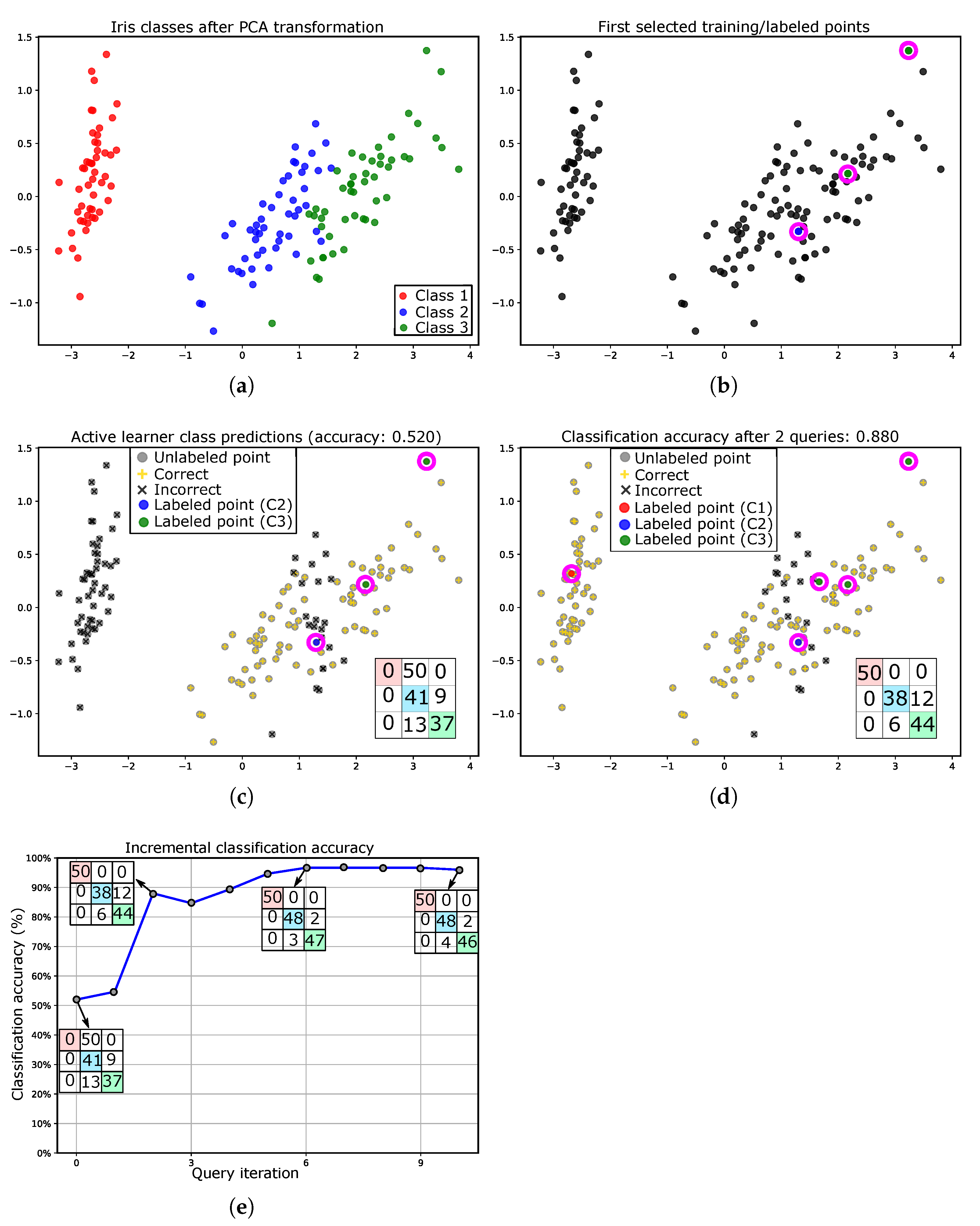
2.3. Illustrative Example

The aim of this example is to explain the idea of the active learning technique. In this example, we use the Iris dataset, which consists of three classes of 50 data points each, where each point is represented by four features. For the purpose of visualization, we used the principal component analysis (PCA) dimensionality reduction technique to reduce the dimensions to only two. Figure 1a shows the original data and Figure 1b shows the data points after hiding their labels; this is the unlabeled data.

First, only three data points were randomly selected and labeled (i.e., their labels made available; see Figure 1c). These initially labeled data represent the initial training data. As shown, the selected points are from only two classes; therefore, the trained model on this training data will classify the test points into two classes. In this example, we used the random forest (RF) learning algorithm, and the test data is the remaining unlabeled data. Figure 1c shows the performance of the trained model with this small training data (only three points), and as shown, the accuracy was only 52% because the small size of the training data causes the model to misclassify all the data points in the first (red) class along with some points in the second and third classes.

Iteratively, in our example, a simple active learner is used to query one of the most uncertain points; this active learner uses the entropy method [10]. As can be seen in Figure 1d, after annotating two points, the accuracy increased from 52% to 88%. This is because one of the newly annotated points belongs to the first class; hence, the current training data includes the three (i.e., all) classes and as shown from the confusion matrix, all points from the first class are correctly classified. Figure 1e shows the classification accuracy during the annotation process, where each point represents the accuracy after annotating a new point. Additionally, the confusion matrix is shown at some points to illustrate the number of correctly classified points from each class. As shown, the accuracy increased to 88% after annotating only two points, one of which belongs to the first class. Furthermore, the accuracy continues to increase as more points are annotated, and as shown, the accuracy is approximately stable after the sixth point. (The code of this example is available at https://github.com/Eng-Alaa/AL_SurveyPaper/blob/main/AL_Iris_SurveyPaper.py or https://github.com/Eng-Alaa/AL_SurveyPaper/blob/main/AL_IrisData_SurveyPaper.ipynb [access date on 28 December 2022]).

This example shows how active learners simply search for highly informative points to label them. This iteratively improves the quality of the labeled/trained data, and, consequently, enhances the accuracy of the learner, which improves the generalizability of the model on data it has never seen before.

2.4. AL Scenarios

There are three main scenarios for ALs:

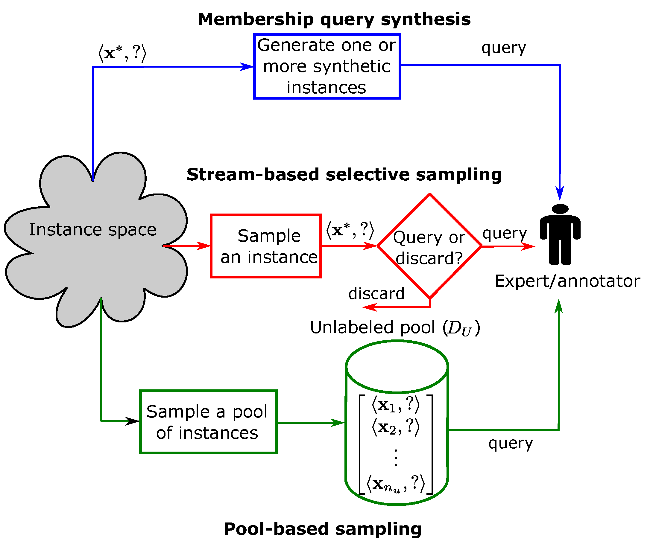
• In the membership query synthesis scenario, the active learner generates synthetic instances in the space and then requests labels for them (see Figure 2). This scenario is suitable for finite problem domains, and because no processing on unlabeled data is required in this scenario, the learner can quickly generate query instances [3]. The major limitation of this scenario is that it can artificially generate instances that are impossible to reasonably label [36]. For example, some of the artificially generated images for classifying handwritten characters contained no recognizable symbols [37].
• In the stream-based selective sampling scenario, the learning model decides whether to annotate the unlabeled point based on its information content [4]. This scenario is also referred to as sequential AL because the unlabeled data points are drawn iteratively, one at a time. In many studies such as [38,39], the selective sampling scenario was considered in a slightly different manner from the pool-based scenario (this scenario is explained below) because, in both scenarios, the queries are performed by selecting a set of instances sampled from a real data distribution, and the main difference between them is that the first scenario (selective sampling) scans the data sequentially, whereas the second scenario samples a large set of points (see Figure 2) [3]. This increases the applicability of the stream-based scenario when memory and/or processing power is limited, such as with mobile devices [3]. In practice, the data stream-based selective sampling scenario may not be suitable in nonstationary data environments due to the potential for data drift.
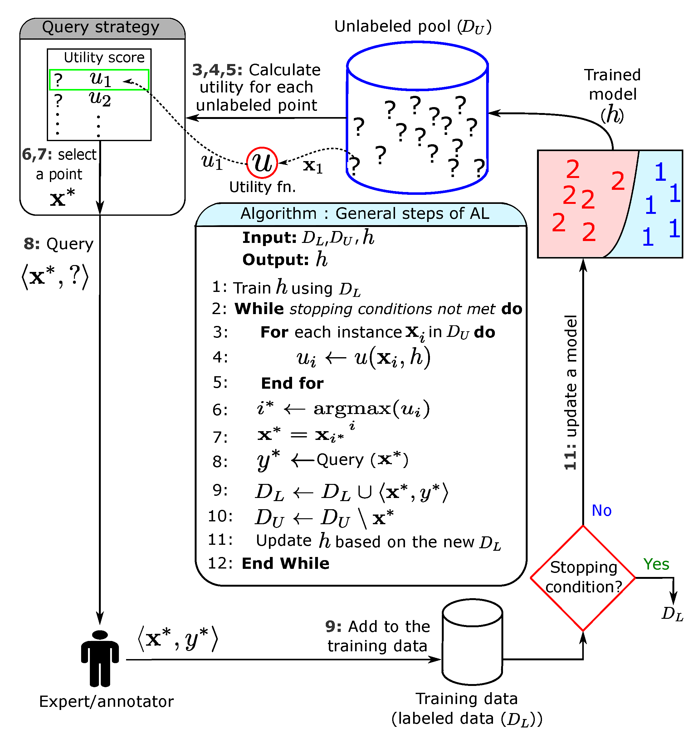
• The pool-based scenario is the most well-known scenario, in which a query strategy is used to measure the informativeness of some/all instances in the large set/pool of available unlabeled data to query some of them [40]. Figure 3 shows that there is labeled data ($D_L$) for training a model (h) and a large pool of unlabeled data ($D_U$). The trained model is used to evaluate the information content of some/all of the unlabeled points in $D_U$ and ask the expert to label/annotate the most informative points. The newly annotated points are added to the training data to further improve the model. These steps show that this scenario is very computationally intensive, as it iteratively evaluates many/all instances in the pool. This process continues until a termination condition is met, such as reaching a certain number of queries (this is called query budget) or when there are no clear improvements in the performance of the trained model.

In some studies, as in [41], the combination of the pool-based and the membership query synthetic scenarios solved the problem of generating arbitrary points by finding the nearest original neighbours to the ones that were generated synthetically.

2.5. AL Components

Any active learner (especially in the pool-based scenario) consists of four main components.

• Data: The first component is the data which consists of labeled and unlabeled data. The unlabeled data ($D_U$) represents the pool from which a new point is selected, and the labeled portion of the data ($D_L$) is used to train a model (h).
• Learning algorithm: The trained model (h) on $D_L$ is the second component and it is used to evaluate the current annotation process and find the most uncertain parts within the space for querying new points there.
• Query strategy: The third component is the query strategy (this is also called the acquisition function [14]) which uses a specific utility function (u) for evaluating the instances in $D_U$ for selecting and querying the most informative and representative point(s) in $D_U$. The active learners are classified in terms of the number of queries at a time into one query and batch active learners.

  –

  One query: Many studies assume that only one query is queried at a time, which means that the learning models should be retrained every time a new sample is added; hence, it is time-consuming [14]. Moreover, adding only one labeled point may not make a noticeable change in the learning model, especially for deep learning and large-scale models.

  –

  Batch query: In [4], the batch active learning technique was proposed. It is suitable for parallel environments (many experiments are running in parallel) to select many samples simultaneously. Simply put, if the batch size is k, a simple active learning strategy could be run repeatedly for k times to select the most informative k points. The problem here is that some similar points could be selected. Therefore, with batch active learning, the sample diversity and the amount of information that each point contains should be taken into consideration.

• Expert: The fourth component is the expert/labeler/annotator/oracle who annotates/labels the queried unlabeled points.

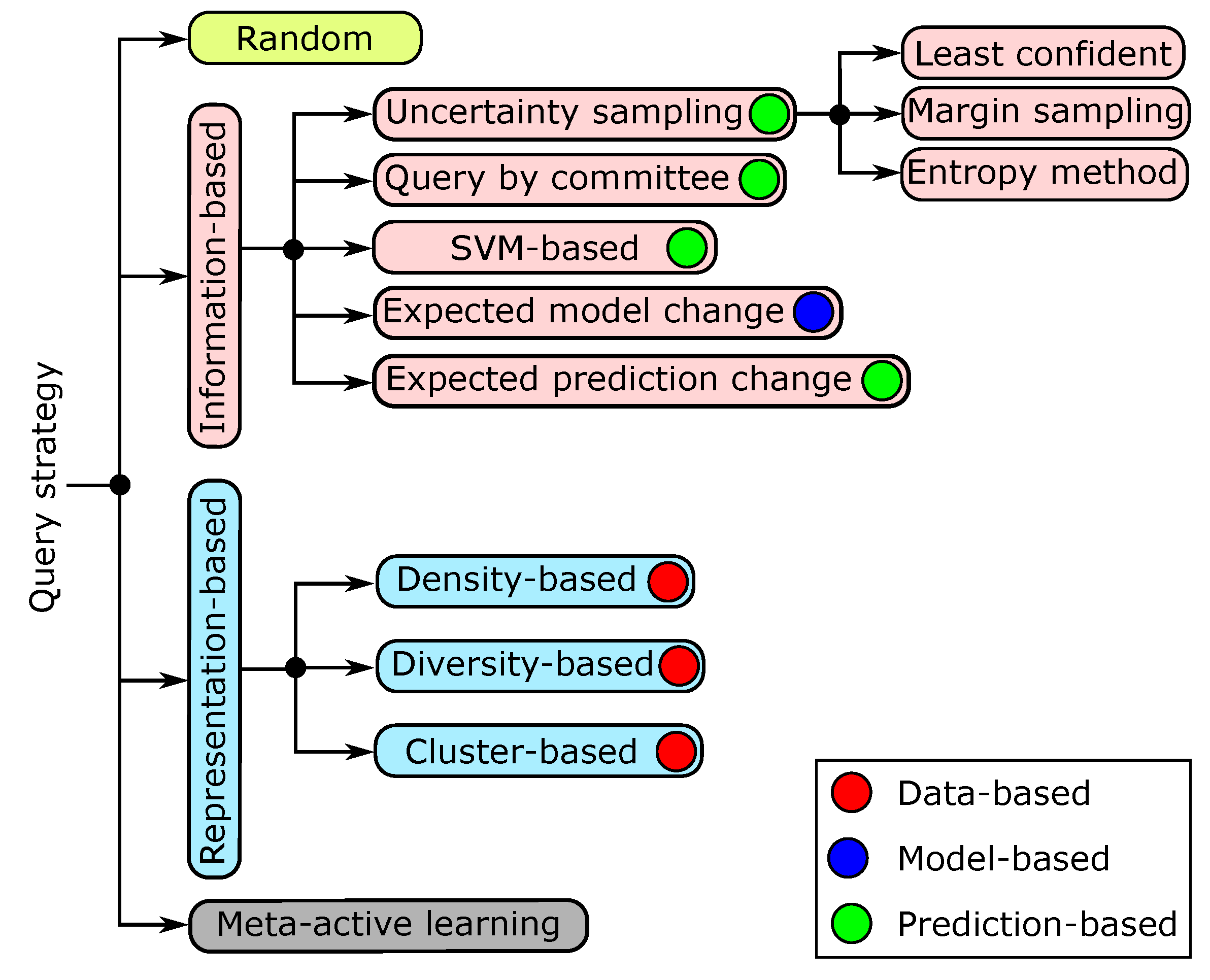
3. Query Strategy Frameworks

The main difference between active learning algorithms is the way a new point is queried, and this is called the query strategy. In each query strategy, a utility function (u) is used for evaluating the instances in $D_U$ and generating utility scores/values. Based on these values, one (or more) point will be selected to be queried. Some active learners search for the most informative points (the ones around the decision boundaries), and this category is called information-based methods (see Figure 4b). Mathematically, this category only takes the uncertainty of the unlabeled instances into consideration; in other words, the utility function is defined as follows, $u=f_u$, where $f_u$ is one of the uncertainty metrics. Another category includes representation-based methods that try to cover the whole input space or the whole unlabeled data without paying attention to critical regions (see Figure 4c). Mathematically, the utility function ($u=q_u$) evaluates the representativeness of the unlabeled points to select the most representative points, where $q_u$ is a utility metric that measures the representativeness of the unlabeled points (e.g., calculating the pairwise correlation between pairs of unlabeled points). As shown in both cases (Figure 4b,c), using only one type (i.e., information-based or representation-based) can cause the learning model to deviate from the true decision boundaries, which reduces classification performance. However, some studies have combined both types. More details are provided in the following sections.

3.1. Information-Based Query Strategies

Active learners in this category search for the most informative points by looking for the most uncertain points that are expected to be close to the decision boundaries. Therefore, as mentioned before, the utility function in this query strategy type calculates only the uncertainty. There are many examples of this category (see Figure 5), which are discussed in more detail in the following sections.

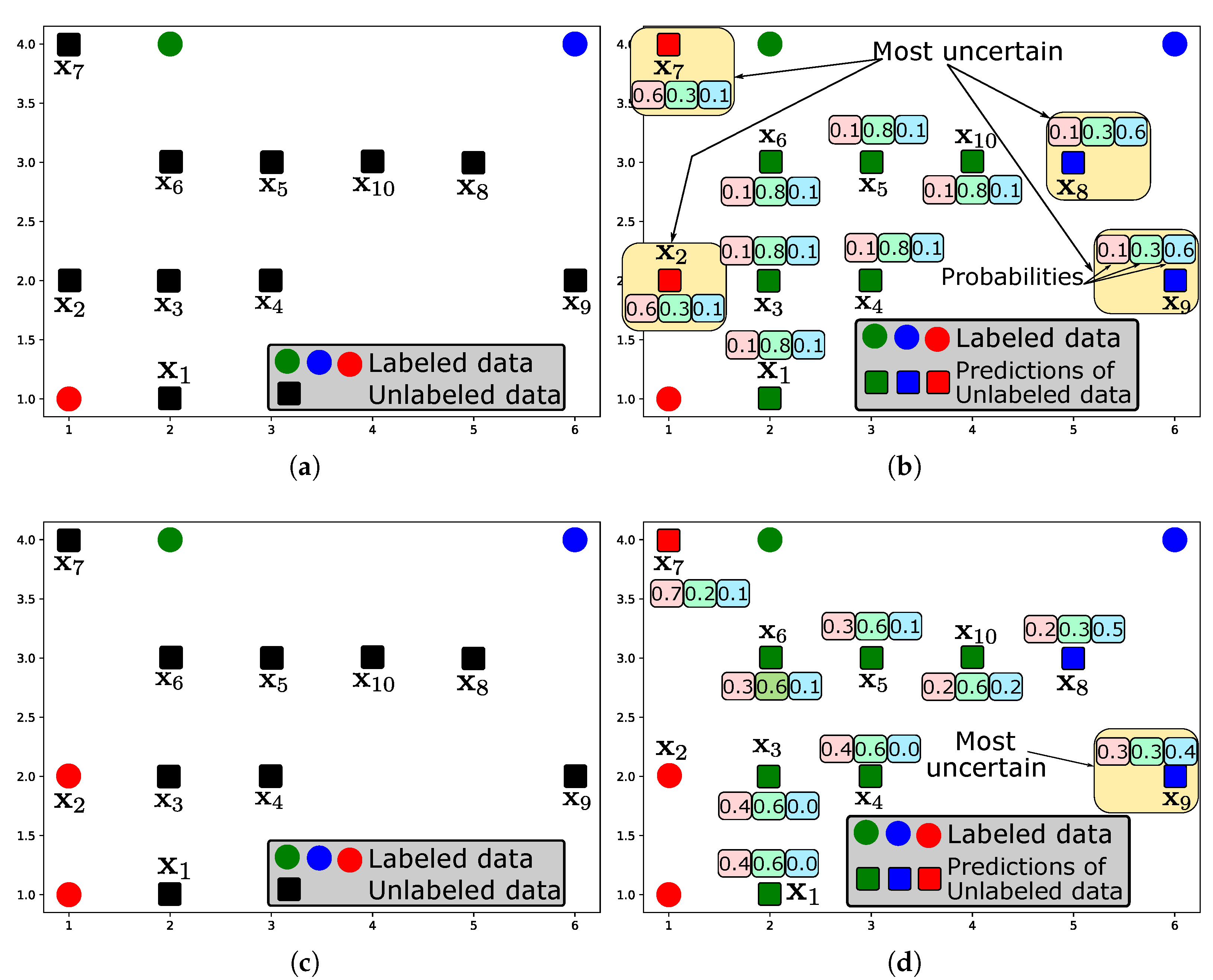
3.1.1. Uncertainty Sampling

Traditional uncertainty sampling methods do not clearly explain the reasons for the uncertainty of the model. In [42], the authors mentioned that there are two reasons for the uncertainty. The first is that the model is uncertain because of strong but conflicting evidence for each class; this is called conflicting-evidence uncertainty. The second type of uncertainty is due to insufficient evidence for either class; this is called insufficient-evidence uncertainty.

In the uncertainty sampling approach, the active learner queries the least certain (or the most uncertain) point; therefore, this strategy is also called the least confident (LC) approach. This strategy is straightforward for probabilistic learning algorithms when in a binary classification problem, the active learner queries the point with a posterior probability of being positive close to $0.5$ [3,40]. The general formula for multi-class problems is

$$\begin{array}{c}\hfill {\mathbf{x}}^{*}=\underset{\mathbf{x}\in D_U}{\mathrm{argmax}}(1-P_h\left(\widehat{y}\right|\mathbf{x})),\end{array}$$

(4)

where ${\mathbf{x}}^{*}$ is the least confident instance, $\widehat{y}=\underset{y}{\mathrm{argmax}}{P}_h\left(y\right|\mathbf{x})$ is the class label of $\mathbf{x}$ with the highest posterior probability using the model h, and $P_h\left(y\right|\mathbf{x})$ is the conditional class probability of the class y given the unlabeled point $\mathbf{x}$. Hence, this method only considers information about the most likely label(s) and neglects the information about the rest of the distribution [40]. Therefore, Schefer et al. introduced the margin sampling method, which calculates the margin between the first and the second most probable class labels as follows [43],

$$\begin{array}{c}\hfill {\mathbf{x}}^{*}=\underset{\mathbf{x}\in D_U}{\mathrm{argmin}}{P}_h\left({\widehat{y}}_1\right|\mathbf{x})-P_h\left({\widehat{y}}_2\right|\mathbf{x}),\end{array}$$

(5)

where ${\widehat{y}}_1$ and ${\widehat{y}}_2$ are the first and second most probable class labels, respectively, under the model h. Instances with small margins are ambiguous, and hence asking about their labels could enhance the model for discriminating between them. In other words, a small margin means that it is difficult for the trained model (h) to differentiate between the two most likely classes (e.g., overlapped classes). For large label sets, the margin sampling method ignores the output distribution of the remaining classes. Here, the entropy method, which takes all classes into account, could be used for measuring the uncertainty as follows,

$$\begin{array}{c}\hfill {\mathbf{x}}^{*}=\underset{\mathbf{x}\in D_U}{\mathrm{argmax}}-\sum _i{P}_h\left(y_i\right|\mathbf{x})\log P_h\left(y_i\right|\mathbf{x}),\end{array}$$

(6)

where $y_i$ ranges over all possible class labels and $P_h\left(y_i\right|\mathbf{x})$ is the conditional class probability of the class $y_i$ for the given unlabeled point $\mathbf{x}$ [44]. The instance with the largest entropy value is queried. This means that the learners query the instance for which the model has the highest output variance in its prediction.

For example, suppose we have two instances (${\mathbf{x}}_1$ and ${\mathbf{x}}_2$) and three classes ($A,B,$ and C) and want to measure the informativeness of each point to select which one should be queried. The posterior probability that ${\mathbf{x}}_1$ belongs to the class $A,B,$ and C is 0.9, 0.08, 0.02, respectively, and similarly, with ${\mathbf{x}}_2$ the probabilities are 0.3, 0.6, 0.1. With the LC approach, the learner is fairly certain that ${\mathbf{x}}_1$ belongs to the class A with probability 0.9, whereas ${\mathbf{x}}_2$ belongs to B with probability 0.6. Hence, the learner selects ${\mathbf{x}}_2$ to query its actual label because it is the least confident. With the margin sampling method, the margin between the two most probable class labels of ${\mathbf{x}}_1$ is $0.9-0.08=0.82$ and the margin of ${\mathbf{x}}_2$ is $0.6-0.3=0.3$. The small margin of ${\mathbf{x}}_2$ shows that it is more uncertain than ${\mathbf{x}}_1$; hence, the learner queries the instance ${\mathbf{x}}_2$. In the entropy sampling method, the entropy of ${\mathbf{x}}_1$ is calculated as $-(0.9{\log }_{2}0.9+0.08{\log }_{2}0.08+0.02{\log }_{2}0.02)=0.5412$, and similarly the entropy of ${\mathbf{x}}_2$ is $1.2955$. Therefore, the learner selects ${\mathbf{x}}_2$ which has the maximum entropy. Therefore, all three approaches query the same instance. However, in some cases, the approaches query different instances. For example, changing the posterior probability of ${\mathbf{x}}_1$ to 0.4, 0.4, 0.2, and of ${\mathbf{x}}_2$ to 0.26, 0.35, 0.39, the LC and entropy methods select ${\mathbf{x}}_2$ whereas the margin approach selects ${\mathbf{x}}_1$. A more detailed analysis of the differences between these approaches shows that the LC and margin methods are more appropriate when the objective is to reduce the classification error to achieve better discrimination between classes, whereas the entropy method is more useful when the objective function is to minimize the log-loss [3,44,45].

The uncertainty approach could also be employed with nonprobabilistic classifiers, such as (i) support vector machines (SVMs) [46] by querying instances near the decision boundary, (ii) NN with probabilistic backpropagation (PBP) [47], and (iii) nearest-neighbour classifier [48] by allowing each neighbour to vote on the class label of each unlabeled point, and having the proportion of these votes represent the posterior probability.

Illustrative Example

The aim of this example is to explain in a step-by-step approach how active learning works (The code of this example is available at https://github.com/Eng-Alaa/AL_SurveyPaper/blob/main/AL_NumericalExample.py and https://github.com/Eng-Alaa/AL_SurveyPaper/blob/main/AL_NumericalExample.ipynb [access date on 28 December 2022]). In this example, there are three training/labeled data points, each with a different color and belonging to a different class, as shown in Figure 6a. Moreover, there are 10 unlabeled data points in black color. The initial labeled points are used for training a learning model (in this example, we used the RF algorithm). Then, the trained model is used to predict the unlabeled points. As shown in Figure 6b, most of the unlabeled points were classified to the green class. In addition to the predictions, the learning algorithm also provides the class probabilities for each point. For example, the class probabilities of the point ${\mathbf{x}}_1$ are 0.1, 0.8, and 0.1, which means that the probability that ${\mathbf{x}}_1$ belongs to the red, green, and blue classes are 0.1, 0.8, and 0.1, respectively. Consequently, ${\mathbf{x}}_1$ belongs to the green class, which has the maximum class probability. Similarly, the class probabilities of all unlabeled points were calculated. From these class probabilities, the four highlighted points were identified as the most uncertain points by using the entropy method, and the active learner was asked to query one of these points. As shown, all the uncertain points lie between two classes (i.e., within the uncertain regions). In our example, we queried the point ${\mathbf{x}}_2$ as shown in Figure 6c. After adding this new annotated point to the labeled data and retraining the model, the predictions of the unlabeled points did not change (this is not always the case), but the class probabilities did change as shown in Figure 6d. As shown, after annotating a point from the red class, some of the nearby unlabeled points are affected, which is evident from the class probabilities of the points ${\mathbf{x}}_1$, ${\mathbf{x}}_3$, and ${\mathbf{x}}_6$, whose class probabilities have changed (compare between Figure 6b and Figure 6d). Finally, according to the class probabilities in Figure 6d, our active learner will annotate the point ${\mathbf{x}}_9$. This process continues until a stopping condition is satisfied.

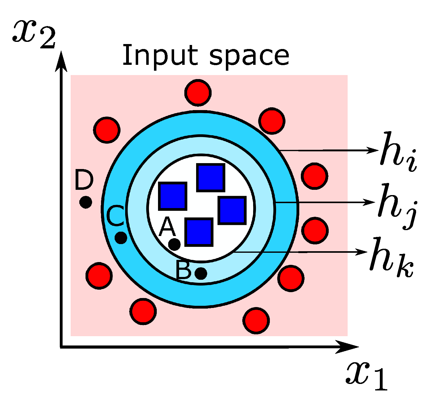
3.1.2. Query by Committee

In the query-by-committee (QBC) approach, a set of models (or committee members) $\mathcal{H}=\{h_1,h_2,\cdots ,\}$ is trained on different subsets of samples drawn from $D_L$ [49]. After that, the disagreement between these committee members is estimated, and then the most informative points are queried where the disagreement between the committee members is the largest. The idea behind this approach is to minimize the so-called version space, i.e., a set of hypotheses that are consistent with the current labeled data ($D_L$). For example, if two hypotheses have been trained and agree on $D_L$ (i.e., both classify the labeled points perfectly, these are called consistent hypotheses), but disagree on some unlabeled points, these points are within the uncertainty region; hence, finding this region is expensive, especially, if it should be maintained after each new query. One famous example of this approach is the committee-by-boosting and the committee-by-bagging techniques, which employ well-known boosting and bagging learning methods for constructing committees [50].

The goal of active learners is to constrain the size of the version space given a few labeled points. This could be done by using the QBC approach by querying controversial regions within the input space. However, there is not yet agreement on the appropriate committee size, but a small committee size has produced acceptable results [49]. For example, in [4], the committee consists of only two neural networks, and it obtained promising results.

Figure 7 shows an example explaining the version space. As shown, with two classes, there are three hypotheses ($h_i$, $h_j$, and $h_k$), where $h_i\in \mathcal{H}$ is the most general hypothesis and $h_k\in \mathcal{H}$ is the most specific one. Both hypotheses ($h_i$ and $h_k$) and all the hypotheses between them including $h_j$ are consistent with the labeled data (i.e., the version space consists of the two hypotheses ($h_i$ and $h_k$) and all the hypotheses between them). Mathematically, given a set of hypotheses $h_i\in \mathcal{H},i=1,2\cdots$, the version space is defined as $V{S}_{\mathcal{H},D_L}=\{h\in \mathcal{H}\mathrm{and}h\left({\mathbf{x}}_i\right)=y_i,\forall {\mathbf{x}}_i\in D_L\}$. Furthermore, as shown, the four points A, B, C, and D do not have the same degree of uncertainty, where A and D are certain (because all hypotheses agree on them, i.e., $h_i$, $h_j$, and $h_k$ classify them identically), whereas B and C are uncertain with different levels of uncertainty. As shown, $h_j$ and $h_k$ classify C to the red class, whereas $h_i$ classifies the same point to the blue class. Therefore, there is a disagreement on classifying the point C. The question here is, how do we measure the disagreement among the committee members?

The level of disagreement among committee members can be measured by many different methods, one of which is the vote entropy method as follows,

$$\begin{array}{c}\hfill {\mathbf{x}}^{*}=\underset{\mathbf{x}}{\mathrm{argmax}}-\sum _i\frac{V\left(y_i\right)}{m}\log \frac{V\left(y_i\right)}{m},\end{array}$$

(7)

where $y_i$ is all possible labels, m indicates the number of classifiers (i.e., number of committee members), and $V\left(y_i\right)$ represents the number of votes that a label receives from the prediction of all classifiers. For example, given three classes (${\omega }_1,{\omega }_2,{\omega }_3$) (i.e., $m=15$), and two instances ${\mathbf{x}}_1$ and ${\mathbf{x}}_2$. For ${\mathbf{x}}_1$, let the votes be as follows: $V(y_1={\omega }_1)=12$, $V(y_1={\omega }_2)=1$, and $V(y_1={\omega }_3)=2$. Hence, the vote entropy of ${\mathbf{x}}_1$ is $-(\frac{12}{15}\log \frac{12}{15}+\frac{1}{15}\log \frac{1}{15}+\frac{2}{15}\log \frac{2}{15})=0.5714$. For ${\mathbf{x}}_2$, let $V(y_2={\omega }_1)=V(y_2={\omega }_2)=V(y_2={\omega }_3)=5$; thus, it is difficult to determine the class label of ${\mathbf{x}}_2$. The, vote entropy of ${\mathbf{x}}_2$ will be $-(\frac{5}{15}\log \frac{5}{15}+\frac{5}{15}\log \frac{5}{15}+\frac{5}{15}\log \frac{5}{15})=1$. Thus, the level of disagreement of ${\mathbf{x}}_2$ is higher than ${\mathbf{x}}_1$, and hence ${\mathbf{x}}_2$ will be selected to be queried (i.e., ${\mathbf{x}}^{*}={\mathbf{x}}_2$).

There are several methods for measuring the disagreement between committee members such as Kullback–Leibler (KL) divergence. This method is always used for measuring the difference between two probability distributions [51]. Here, with AL, the most informative point is the one with the largest average difference (i.e., disagreement) between the label distributions of all committee members [3]. Furthermore, Melville et al. used the Jensen–Shannon divergence and Körner employed the Korner–Wrobel disagreement measure for measuring the disagreement [52,53].

3.1.3. SVMs-Based Approach

SVMs learn a linear decision boundary that has the maximum distance between the nearest training points from different classes [54]. The idea of SVM could be used for reducing the version space by trying to query points near the separating hyperplane. For example, the simple margin method queries the nearest unlabeled point that simply maximally divides the version space [13]. In some studies, SVM has been used to build active learners. For example, in the MaxMin margin method, for binary classification problems, SVM is run twice for each unlabeled point, the first run assuming that the unlabeled point belongs to the positive class and the second run assuming that the point belongs to the negative class [46,55]. The learner checks the margins in both cases ($m_i^{+},m_i^{-}$), and the AL queries the point that maximizes the value of $\min (m_i^{+},m_i^{-})$. The ratio margin method is also very similar, and it maximizes the value of $(\frac{m_i^{-}}{m_i^{+}},\frac{m_i^{+}}{m_i^{-}})$ [13,55,56].

3.1.4. Expected Model Change

This strategy queries the points that produce the largest change in the current model. In other words, the active learner queries the points that are expected to have the greatest impact on the model (i.e., the greatest influence of its parameters), regardless of the resulting query label. One example is the expected gradient length (EGL) method [57], because it can be applied to many learning problems, and the gradient-based optimization algorithms are already used for training learning models [44]. Another example is the expected weight change [58]. However, as reported in [3], this strategy is very computationally intensive, especially for problems with high dimensionality and/or large labeled data. Additionally, the performance of this strategy is severely degraded when the features are not scaled.

3.1.5. Expected Error/Prediction Change

With this strategy, the active learners estimate the expected future error of the trained model by using $D_L\cup 〈{\mathbf{x}}^{*},y^{*}〉$ on the remaining unlabeled data ($D_U$) and then query the points that reduce the expected future error [59], for example, minimizing the expected $0/1$-loss as follows,

$$\begin{array}{c}\hfill {\mathbf{x}}_{0/1}^{*}=\underset{\mathbf{x}}{\mathrm{argmax}}\sum _i{P}_h\left(y_i\right|\mathbf{x})\left(\sum _{j=1}^{n_u}1-P_{h^{+〈{\mathbf{x}}^{*},y^{*}〉}}\left(\widehat{y}\right|{\mathbf{x}}^{\left(j\right)})\right),\end{array}$$

where $P_{h^{+〈{\mathbf{x}}^{*},y^{*}〉}}$ is the new model after retraining it with $D_L\cup 〈{\mathbf{x}}^{*},y^{*}〉$. Therefore, a validation set is required in this category for evaluating the performance of the learned hypotheses. Initially, an initial hypothesis is trained on the available labeled data. Next, the trained model selects a point from the unlabeled pool, labels it, and then adds it to the labeled data. After that, the hypothesis is retrained by using the updated set of labeled data. This process is repeated by assigning the selected point to all possible classes to calculate the average expected loss. This active learning strategy was employed in [59] for text classification. However, because this strategy iteratively retrains the model after labeling each new point, it requires a high computational cost. Moreover, calculating the future error over $D_U$ for each query dramatically increases the computational costs.

Another variant of this strategy is the variance reduction method [3]. In this method, active learners query points that minimize the model’s variance, which consequently minimizes the future generalization error of the model. This method is considered a variant from the expected error reduction because minimizing the expected error can be interpreted as a reduction of the output variance.

3.1.6. Challenges of Information-Based Query Strategies

As we mentioned before, this category of query strategies searches only for the points around the decision boundaries, without considering the whole input space and the spread of the data [12]. Because the points are selected independently, many similar instances could be selected from a small range of the input space, leading to redundancy in the generated labeled set (see Figure 4b). Furthermore, focusing on selecting highly informative points could result in selecting some outliers that are close to the decision boundary, therefore wasting the query budget without providing any real improvement to the learning model. Furthermore, most active learners in this category rely on machine learning models for finding critical regions or quantifying the uncertainty of unlabeled points; these machine learning models are strongly affected by (i) initial training data or general initial knowledge (e.g., the number of classes or the majority and minority classes), and (ii) their parameters that should be tuned. Hence, small initial training data that do not contain enough information may cause the machine learning model to extrapolate (make predictions for data that are outside the range of the training data), resulting in incorrect calculation of disagreement or uncertainty scores.

3.2. Representation-Based Query Strategies

In this category, the active learners try to use the structure of the unlabeled data to find some points that represent the structure of the whole input space. Therefore, the utility function in this category measures the representativeness of the points in $D_U$ to query the most representative ones. The representation-based approach has the advantage over the information-based approach in that it queries points in dense regions, which increases the exploration performance of this approach. This is especially true at the beginning of the learning process when only a few labeled points are available; here, the induced models tend to be less reliable; consequently, their contribution to the AL process is unstable. On the other hand, the information-based approach has the advantage of finding uncertain and critical regions in the search space and exploring them by annotating new points. The next sections explain several approaches of the representation-based query strategy.

3.2.1. Density-Based Approach

In this strategy, representative points are retrieved by querying instances from regions with high density within the input space. Several methods are used for measuring the representativeness of the points. The most widely used are the similarity-based methods such as the distance between feature vectors. For example, Wu et al. selected the unlabeled point that has the minimum distance to all other remaining unlabeled points [60]. Some similarity-based techniques use the correlation between feature vectors, which can also be used to measure the representativeness of the selected points. For example, in [12], cosine similarity, KL divergence, and Gaussian similarity have been discussed for selecting representative points.

3.2.2. Cluster-Based Approach

Clustering methods can be used to select representative points [61]. Here, after clustering the whole input space, the nearest neighbours to the clusters’ centres are selected; hence, the performance of this method mainly depends on the chosen clustering technique and its parameters. This method was applied in text classification in [62].

3.2.3. Diversity-Based Approach

This approach was introduced in [63] for solving a problem that appears when working in parallel environments to speed up the labeling process. The problem is that the same instances are queried, leading to redundancy in the selected points. This approach tries to solve this problem by querying the unlabeled point that has more diversity than the other labeled points. This diversity could be estimated simply by calculating the angles between the feature vector of the selected unlabeled point and the feature vectors of all points in $D_L$. The unlabeled point is selected and queried if it is sufficiently different/diverse from the other points in $D_L$. However, trying to maximize the diversity among labeled points may result in querying some outliers; therefore, it was recommended in [13,64] to combine this method with some other methods to achieve better performance.

3.2.4. Challenges of the Representation-Based Strategies

The selection of instances representing the structure of the input space increases the quality of the selected points and ensures that the selected points are not concentrated only in a small region, as in the information-based strategy. Significantly, this strategy tackles the problem of querying outliers much better than the information-based query strategy. Furthermore, this query strategy removes the problems of sampling bias and selecting redundant points by covering different regions within the input space. However, selecting representative points may require more queries to cover all uncertain regions in the space that should be covered. This makes the convergence to high classification accuracy slower than the information-based query strategy.

3.3. Informative and Representative-Based Query Strategies

Several studies have combined the two aforementioned strategies (i.e., the informative-based and the representative-based) to obtain high-quality labeled data (i.e., the utility function will be $u=f_u\times q_u$) [65,66]. For example, in [44], the QBC method was employed for querying the most informative points and the similarity-based method was used for finding the most representative points. In another example, the cluster information of the unlabeled data was combined with the classification margins of a statistical model [67]. In [68], for object classification, the exploration and classical exploitation methods were combined. In the exploration phase, with no initial labeled data and no need to compute similarity to all points, the active learner searches for the most representative points by computing the potential of each unlabeled data point and selecting the point with the highest potential. In [69,70], with the aim of exploring the subspaces of minority classes in imbalanced data problems, a novel model was introduced that attempts to balance the exploration and exploitation phases. However, most techniques that combine informative and representative points sometimes result in suboptimal performance [71]. This is because, to our knowledge, it is still a challenge to effectively combine both strategies.

3.4. Meta-Active Learning

The performance of active learning depends mainly on the prediction model, data distribution, and the compatibility of the acquisition function to them. Therefore, changing any of these factors changes the overall performance of the active learner. Here, another recent technique makes the acquisition function flexible by updating itself and learning from data by formulating the active learning problem in the reinforcement learning framework, where the acquisition function is expressed as a policy to be learned by reinforcement learning [14,72,73].

For example, in [74], the stream-based active learning scenario was considered as a Markov decision process and proposed to learn the optimal policy by setting the parameters of the prediction model and considering a state as an unlabeled data point and the action as whether a label is required. Moreover, deep reinforcement learning with long short-term memory (LSTM) was used in [75] to design a function that determines if a label of a data point needs to be queried for stream-based active learning. Here, the Q-function is used to determine the value of an action in a certain state, and to take a decision on whether to label this unlabeled point. In another example in [76], the deep reinforcement learning technique was employed for designing the acquisition function that is updated dynamically with the input distribution. Recently, the problem of finding the optimal query is closely related to the bandit problem, and in [77,78,79], the acquisition function was designed as a multi-armed bandit problem.

3.5. Other Classifications of AL

In [26], query strategies are classified by the amount of information available into the following categories:

• Random: This is the most well-known and traditional method in which unlabeled points are queried randomly (i.e., this category does not use any knowledge about data or models).
• Data-based: This category has the lowest level of knowledge and works only with the raw data and the labels of the current labeled data. This category could be further divided into (i) strategies that rely only on measuring the representativeness of the points (i.e., representation-based) and (ii) strategies that rely on the data uncertainty by using information about data distribution and the distribution of the labels.
• Model-based: This category has knowledge about both the data and the model (without predictions). One clear example is the expected model change, where after training a model using some labeled points, the model queries a new unlabeled point that obtains the greatest impact on the model (e.g., model’s parameters such as expected weight change [58] and expected gradient length [57]), regardless of the resulting query label.
• Prediction-based: All types of knowledge are available in this category (from data, models, and predictions). A well-known example is the uncertainty sampling method, in which a new point is selected based on the predictions of the trained model. The most uncertain unlabeled point will be queried. However, there is a thin line between the model-based and prediction-based categories. In [26], it was mentioned that the prediction-based category searches for interclass uncertainty (i.e., the uncertainty between different classes), whereas the model-based category searches for intraclass uncertainty (i.e., the uncertainty within a class).

In [17], query strategies were classified into the following categories:

• Agnostic strategies: This approach makes no assumption about the correctness (or how accurate) of the decision boundaries of the trained model. In other words, this approach ignores all the information generated by the learning algorithm and uses only the information from the pool of unlabeled data. Therefore, this approach could be approximately the same as the representation-based approach in our classification.
• Nonagnostic strategies: This approach mainly depends on the trained model to select and query new unlabeled points. Therefore, this approach is very similar to the information-based approach we presented earlier.

4. Practical Challenges of AL in Real Environments

Despite the fact that AL reduces the number of labeled points required for obtaining promising results, it still has some challenges.

4.1. Noisy Labeled Data

A noisy data point is a point that is mislabeled (i.e., it has an incorrect ground truth). Therefore, noisy labeled data contaminates the training data and has a negative impact that can be more harmful than just having small training data. There are many reasons for these noisy points, such as some experts’ carelessness or accidental mistakes in labeling. Another reason is that some experts have insufficient knowledge for labeling new data points, due to the lack of data from a certain class or when the unlabeled instances contain limited information (e.g., unclear images) [80]. Furthermore, the drift in data may change the posterior probability of some classes, which changes the class labels of some historical labeled data points; hence, these points become noisy-labeled.

One of the trivial solutions for handling the noisy data problem is to relabel these noisy points again by asking many weak labelers (nonexperts or noisy experts) who might return noisy labels as in [81,82,83]. This relies on the redundancy of queried labels of noisy labeled points from multiple annotators, which certainly increases the labeling cost. For example, for an expert, if the probability to annotate some points incorrectly is 10%, with two annotators, this drops to $0.1\times 0.1=0.01=1\%$, which is better and may be sufficient in some applications. However, repeatedly asking experts for labeling some instances over multiple rounds could be an expensive and impractical solution, especially if the labelers should be experts, such as in medical image labeling, or if the labeling process is complicated [84]. The noisy labeled data problem could also be solved by modelling the expert’s knowledge and asking the expert to label an instance if it belongs to his knowledge domain [85]. If the expert is uncertain about the annotations of some instances, the active learner can accept or reject the labels [86]. However, for real challenges such as concept drift, imbalanced data, and streaming data, it may be difficult to characterize the uncertain knowledge of each expert. There are many reasons for this, e.g., each expert’s uncertain domain may change due to drift. In [87], with the aim of cleaning the data, the QActor model uses a novel measure CENT, which considers both the cross-entropy and the entropy measures to query informative and noisy labeled points.

There are still many open research questions related to noisy labeled data [82]. For example

RQ1: What happens if there are no experts who know the ground truth? and

RQ2: How might the active learner deal with the other experts whose quality fluctuates over time (e.g., at the end of a long annotation task)?

4.2. The Imbalanced Data Problem

The problem of imbalanced data is one of the well-known challenges in many applications. For example, faulty instances are rare compared to normal instances in industrial applications, and furthermore, some faulty classes are very small compared to other faults (i.e., they rarely occur) [88]. The impact of this problem increases with the drift and continuity of the data, which reduces the chances of obtaining instances from the minority classes. Consequently, active learners should improve their exploration ability to cover the whole space and find part of the minority class, especially when the imbalance ratio (the ratio between the number of majority class instances and the number of minority class instances) is high. This is one of the trivial research questions here:

RQ3: How AL can deal with imbalanced data with severe imbalance ratios?

Many studies, such as [77,88], did not take the imbalanced data problem into consideration. On the other hand, many active learners try to handle the imbalanced data by employing the commonly used sampling algorithms for obtaining balanced data. For example, the Learn++.CDS algorithm used the synthetic minority oversampling technique (SMOTE) algorithm for balancing the data [89]. Oversampling and undersampling bagging were also presented in [90,91]. With nonstationary environments, in [92], the minority instances from previous batches were propagated whereas the majority points of the current batch were undersampled. This was enhanced in [93] by selecting only the minority points that were similar to the current batch.

While many studies have presented solutions to the problem of imbalanced data, to our knowledge they have not attempted to detect the presence of imbalanced data. Instead, they initially assumed that the data is imbalanced and also that the minority class(es) is known. Therefore, in practice, active learners should be designed more flexibly to solve the problem of imbalanced data adaptively and without using prior knowledge. Hence, one of the research questions here is

RQ4: How could the active learner be more flexible to adapt to new data with new classes that might be small compared to other classes?

As far as we know, the authors in [69,70] have introduced active learners that adapt themselves to imbalanced and balanced data without predefined knowledge, and they have achieved promising results.

4.3. Low Query Budget

One of the biggest challenges with many active learners is that they need to query a large portion of unlabeled data to achieve acceptable results. In practice, the query budget in many applications should be small due to the cost and time involved in labeling, especially when data is arriving continuously and rapidly in streams. Therefore, labeling a large number of points might be impractical [94]. For example, the budget was 20% in [95], was ranging from 15% to 40% in [96], and reached 80% in [67] of the total number of unlabeled points. Furthermore, with high-dimensional data, most of the deep learning active learners need large initial labeled data and a high query budget for optimizing their massive number of parameters [97]. However, with a small query budget, it is difficult to extract enough information to learn a predictive model with low error rates, especially, with high-dimensional data problems; this is one of the main research questions:

RQ5: How can active learners achieve promising results with a small query budget?

4.4. Variable Labeling Costs

In many applications, not only the quality of labeling varies from one point to another, but also the labeling costs, which are not always the same for all data points. Some studies assume that the cost of labeling normal and defective products in industrial environments is the same. However, as reported in [13], because the misclassification error changes from one class to another, labeling costs should also be different. Therefore, a reduction in the query budget does not necessarily guarantee a reduction in the overall cost of labeling. For example, Tomanek et al. considered that the labeling cost is estimated based only on annotation time [98]. Settles, in [99], mentioned that labeling time mainly depends on the expert’s skill, which changes from one to another, so we cannot consider only the labeling time. In [100,101], the cost of mislabeling in intrusion-detection systems was combined with the cost of instance selection, resulting in different labeling costs. In summary, one of the key research questions here is

RQ6: How do we calculate the labeling costs in some applications? In addition,

RQ7: Are the labeling costs of instances from different (or similar) classes similar/identical?

4.5. Using Initial Knowledge for Training Learning Models

Many (or the majority) of active learners assume that there is some initial knowledge, which helps to initialize and build the active learner (e.g., initial labeled data), and pass some guided notes to the active learner such as the number of classes, presence of imbalanced data, and the majority and the minority classes. This initial knowledge adds many limitations in addition to increasing the required cost and time for the labeling process. One of these limitations is that the initial training data are selected and queried randomly from the unlabeled data. Thus, the size of this training set and the selected points have an impact on the behavior and the overall performance of the active learners. Furthermore, annotating points from all classes is difficult with imbalanced data, especially, with severe imbalance ratios. Additionally, assuming that the number of classes is fixed reduces the flexibility of the models, because these models cannot cope with the applications that have a variable number of classes. Without a detection step, the assumption that (i) the data are imbalanced and (ii) the majority and minority classes are known is helpful in fitting a model, but this assumption, which is not always available, makes the model inflexible in many situations (e.g., when this knowledge about the data is not available or when new classes may appear over time). Therefore, an important research question here is

RQ8: How could AL be implemented with no (or little) initial knowledge?

However, most of the current active learners consider that initial knowledge is available. For example, active learners in [41,95,96,102] require initial labeling points, and the models in [41,96,102,103,104] were initialized with the number of classes, and some of them only handle binary classification data. In addition, some active learners only work under the condition that they have initial labeled points from all classes. For example, the initial training data in [105] should contain 15 instances from each class, and even if the data is expected to be imbalanced, the initial training data should also contain points from the minority classes [41,102]. However, some recent studies have taken this problem into account and introduced novel active learners that do not require prior knowledge [69,70].

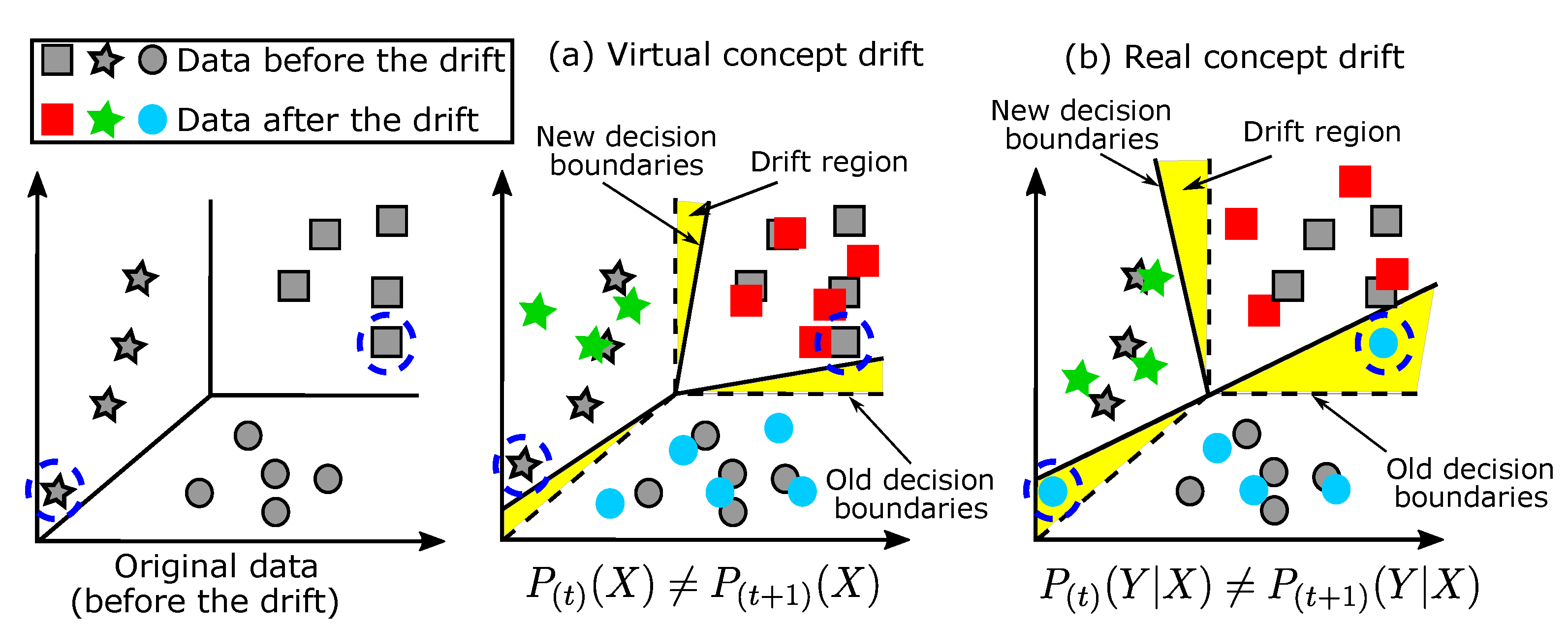
4.6. The Concept Drift Phenomenon in Data Streams

In real-world environments, the streams of data are collected continuously, here, the labeling process is more challenging due to the large amount of data and the pool is not static. Furthermore, the data distribution could be changed over time, which is referred to as concept drift. For example, in a production line, one or more sensors may be repaired, replaced, or manually adjusted over time, changing the attributes of faulty and normal data points [95]. This drift in the newly received data may change the conditional class probabilities without affecting the posterior probabilities; this is referred to as virtual drift, wherein the decision boundaries are shifted slightly but without changing the class labels of the historical data. In contrast, real drift changes the posterior probabilities of some classes; consequently, this updates the decision boundaries and class labels of some patterns (see Figure 8). Therefore, some instances of the historical data become irrelevant or even harmful to the current trained models that were trained with the old/historical data [106]. This means that two identical points labeled before and after data drift may belong to two different classes; this negatively affects both passive and active learners. Therefore, this drift should be recognized and addressed.

There are many methods to detect the drift. The simplest method is to periodically train a new model by using the most recently obtained data and replace the old model; these methods are called blind methods. However, it is better to adjust the current model than to discard it completely. Therefore, in some studies, the drift detection step has been incorporated into active learners to monitor the received data and check if the data distributions change with the data stream [107]. In [108], the adaptive window (ADWIN) method compares the mean values of two subwindows; drift is detected when these subwindows differ significantly enough. The drift can also be detected from the results of the learning models [109], such as the online error rate, or even from the parameters of the learning models [110]. After detecting the drift, some of the historical data should be removed, whereas the others are kept for revising the current learning model if a remarkable change is detected, and the current learning model should be adapted to the current data, for example, by retraining it by using the new data. In some studies, many adaptive ensemble ML algorithms are used to deal with the concept deviation by adding/removing some weak classifiers. For example, in [111], the dynamically weighted majority (DWM) model reduces the weight of a weak learner that misclassifies an instance and removes the weak learners whose weights are below a predefined threshold. In another example, in [89], the weak learners are weighted according to the prediction error rates of the latest streaming data, and the weak learners with low error rates are replaced with new ones. However, detecting drift in real environments and adjusting the model during drift is still an open question (RQ9), especially in real environments that present other practical problems.

4.7. AL with Multilabel Applications

It is usually assumed that each instance has only one class label, whereas in practice, in some cases, the instance could have many labels at a time [112,113]. For example, an image could be labeled with several labels [113]. However, acquiring all labels of even a small set of points increases the labeling cost dramatically. Moreover, in most cases, the relationships between labels (i.e., label correlation) are ignored. Another challenge also is the measuring of informativeness of the unlabeled data points across all labels. One of the solutions was to decompose the multilabel classification problem into a set of binary classification problems, and this is called problem transformation [114]. In another study, Reyes et al. introduced two uncertainty measures based on the base classifier predictions and the inconsistency of a predicted label set, respectively, to query the most informative points, and the rank aggregation technique was used for finding the scores across all labels [115].

4.8. Stopping Criteria

In the active learning technique, the query process continues until a stopping condition is met. As reported in [116], setting an appropriate termination condition for active learners is a tradeoff between the labeling cost and the efficiency of the learning algorithm. In ALs, there are several stopping/termination conditions. One of the most well-known is the query budget or label complexity [14] (i.e., the percentage of the total number of unlabeled points), where the learner iteratively queries unlabeled points until it reaches this budget. This means that the learner will continue to query points even if the learner’s accuracy is sufficient or constant. In contrast, the self-stopping methods might stop querying points when the learner’s accuracy reaches a plateau (this is called sample complexity [14]); therefore, querying more points is likely to be a waste of resources. The active learner could also be stopped when no more informative data points are available [117]. In practice, because it is difficult to specify a priori the size of the training data or the desired level of performance, it is more appropriate to use a predefined uncertainty threshold, where the active learner stops when the level of uncertainty is below a predefined threshold; this was introduced in [118], by introducing a novel uncertainty-based stopping condition; analyzing the proportion of the epistemic uncertainty that reflects the learner’s knowledge. The active learner could thus be stopped if the epistemic uncertainty observed during the annotation process did not change. In another study, based on the confidence estimation over the unlabeled data, four different stopping conditions were introduced in [116], namely maximum uncertainty, overall uncertainty, selected accuracy, and minimum expected error methods. These methods with a threshold value at each method were used as the termination condition, this threshold value was updated elastically during the annotation process, which makes the termination condition flexible and can also be updated dynamically. Because there are many methods to quantify uncertainty and some of them are mainly based on ML models, the following question arises:

RQ10: In which way we can quantify uncertainty to obtain an indicator of the termination condition of AL?

4.9. AL with Outliers

Outliers are data points (or instances) that have significant deviations from the average value of the entire data. Data with outliers can affect active learners if some of these outliers are selected and queried. Querying these outliers wastes labeling costs by exploring regions that are far from normal data, which negatively affects the overall performance of the active learner. One solution to this problem is to detect outliers and remove them from the pool of unlabeled data, or at least avoid querying them [119]. This could be done by detecting the outliers geometrically [120]. However, as reported in [121], if the data is imbalanced with a strong imbalance, the minority class (or part of it) can be considered as an outlier; therefore, filtering out or removing the outliers is not always the best option. Another solution to the outlier problem is to combine information-based and representation-based methods as in [70]. This is because, as mentioned earlier, information-based active learners can select some outliers that are close to the decision boundary. On the other hand, in representation-based active learners, the presence of outliers is less problematic. Therefore, the combination of both methods could be a solution to the problem of outliers. In summary, this problem is still an open research question, namely

RQ11: How could the active learning technique handle the presence of outliers?

4.10. AL in High-Dimensional Environments

Most classical active learners work only in low-dimensional environments as in [46,122]. This is because, with a low query budget, it is not sufficient to train a model with data that has high dimensionality. Practically, this is always one of the main research questions, namely.

RQ12: How does AL with a low-query budget behave in high-dimensional spaces?

Recently, because the format of collected data such as images, videos, and text are high-dimensional, deep learning technology has been combined with active learning. This is called deep active learning (DAL) [97]. Here, as mentioned in [46], a huge amount of data is required to train DL models with thousands of parameters. However, many methods are used to add some extra supervised knowledge such as adding some pseudolabels [123] and generating high-quality synthetic data [124].

4.11. ML-Based Active Learners

One of the main challenges is that the labeled data (i.e., the training set) has already been created in collaboration with an active learner who is heavily influenced by the ML model used for query selection. Therefore, a change in the model leads to a change in the selected queries and consequently in the labeling set [3]. In other words, the selected training data points are a biased distribution [3]. This might be the reason why some studies report that active learners perform better when using random sampling; in other words, active learners need more labeled data than passive learners to achieve the same performance [45,125]. On the other hand, fortunately, some studies have demonstrated that labeled data selected by an algorithm (e.g., naive Bayes in [126]) produces promising results with other learners (e.g., decision tree classifiers in [126]). Another important point is that the learning model tends to extrapolate when the number of initial training data is small, leading to the incorrect calculation of disagreement or uncertainty scores. Furthermore, the performance and behavior of ML mainly depend on the initial training data, which increases the labeling cost. Moreover, changing the initial training data changes the performance of ML models, which is a sign of the instability of ML-based active learners. Furthermore, ML models are also strongly influenced by their parameters, which should be tuned. All these problems related to ML-based active learners motivate us to ask the following research question:

RQ13: Can AL find uncertain regions without using ML models?

4.12. AL with Crowdsourcing Labelers

Due to the high cost of the labeling process, crowd labeling (or noisy labelers) is one of the solutions, wherein instances are labeled by workers (not experts) whose suggestions are not always correct. Recently, it has become common to annotate visual datasets on a large-scale by using crowd-sourcing tools such as Amazon Mechanical Turk [127]. As a result, the annotations collected can be very noisy. To improve the annotation process for visual recognition tasks, in [128], the expertise of noisy annotators is modelled to select high-quality annotators for the selected data. Another solution is to discard the labels of the labeler who always disagrees with the majority of the other labelers [129]. In [130], a novel positive label threshold (PLAT) algorithm was introduced to determine the class membership of many noisy labelers for each data point in a training set. This yielded promising results even for unbalanced data.

5. AL with Different Technologies (Research Areas)

5.1. AL with Deep Learning

Simply put, deep learning (DL) technology is a class of ML technology that uses artificial neural networks (ANN) in which multiple consecutive layers are used for extracting higher-level features from the input data. For optimizing the massive number of parameters of DL algorithms, a large amount of training data is required for extracting high-quality features [97]. Despite this, DL has made a breakthrough in many fields in which large public datasets are available. However, due to the labeling cost, collecting enough data for training DL algorithms is still challenging. Here, AL offers a solution by labeling small and high-quality training data; this combination (i.e., DL and AL) is called deep AL (DAL). This combination has many challenges. The main challenge is the initially labeled data, which in many cases is not sufficient for learning and updating DL models. Many solutions are used to solve this problem such as (i) using generative networks for data augmentation [124], (ii) assigning pseudolabels to high-confidence instances to increase the amount of labeled data [123], and (iii) combining both labeled and unlabeled data by combining supervised and unsupervised training during AL cycles [131,132]. Moreover, the one-by-one annotation approach of some active learners is not applicable in the DL context; therefore, approximately all DAL studies use batch query strategies instead of one query [133]. This increases the chance of selecting representative points [134]. Another challenge is that because DL could use the softmax layer for obtaining the probability distribution of the labels, as reported in [97], the softmax response of the final output is unreliable [135]; then, it could not be used for finding uncertain patterns, and as reported in [123], the performance might be worse than using random sampling. This problem was solved by applying Bayesian deep learning [136] in order to deal with the high-dimensional mini-batch samples with AL that use fewer queries [137,138]. One of the practical challenges in combining DL and AL is that the processing pipelines of AL and DL are inconsistent. This is because AL used fixed feature representations with a focus on the training of classifiers. However, in DL the steps of feature learning and classifier training are jointly optimized. Therefore, different studies treated them as two separate problems or only fine-tuning the DL models within the AL framework [123].

5.2. Few-Shot Learning with AL

The strategy of “few-shot learning” (FSL) (or “low-shot learning” (LSL)) is a subset of machine learning in which experience is gained not only from the hard-to-gather training data but from a very small training/labeling set (called the “support set”) and some prior knowledge. This prior knowledge could be similar datasets or a pretrained model on similar datasets [2]. The active learning strategy could be used here for providing feedback from experts which improves the accuracy of FSL. In [139], a semisupervised few-shot model was introduced, in which the prototypical networks (PN) are used for producing clustered data in the embedding space, but the initial prototypes are estimated by using the labeled data. Next, one of the clustering algorithms such as K-means is then performed on the embeddings of both labeled and unlabeled data. AL was employed for reducing the errors due to the incorrect labeling of the clusters [139,140]. In [75], reinforcement learning and one-shot learning techniques are combined to allow the model to decide which data points are worth labeling during classification. AL was combined with zero-shot learning, where without using the target annotated data, the zero-shot learning uses the relation between the source task and target one for predicting the label distribution of the unlabeled target data [141]. The obtained results act as prior knowledge for AL.

5.3. Active Data Acquisition

For some applications, collecting all (or sufficient) features is expensive, time-consuming, and may not be possible. For example, medical diagnostic systems should have access to some patient data, such as some symptoms, but not all symptoms, especially those requiring complex procedures [3]. Therefore, adding additional features may require performing additional diagnostic procedures. In this case, the learning model learns from an incomplete feature set. In such domains, the active learning feature acquisition technique is asking/requesting more feature information. Thus, instead of searching for informative points as in classical AL, the AL feature acquisition technique searches for the most informative features [142]. For example, in [143], features can be obtained/collected during classification and not during training.

In industry, there are two main types of inspection: low-cost basic inspection and expensive and time-consuming advanced inspection. All products are inspected by using baseline inspections to train a model that predicts defects in final products. Here, AL could be used to build active inspection models that select some points (products) in uncertain regions to further investigate them with advanced inspections [144].

5.4. AL with Optimization

In evolutionary optimization algorithms, with high-dimensional search space, the number of fitness evaluations increases dramatically, which increases the overall fitness evaluations until finding the optimal solution. Additionally, with expensive problems (i.e., each fitness evaluation is expensive and/or requires more time), finding the optimal solution is also expensive [145]. ML offers a solution by building a surrogate model that will be used for evaluating some solutions instead of relying on using the original fitness function. Active learning could be used here for saving the number of fitness evaluations. This could be shown in Figure 9 by first evaluating some initial points by using the original fitness function. Next, these initial points paired with their fitness values are used as training data for training a surrogate model, which tries iteratively to approximate the original fitness function. As shown in Figure 9a, four initial points are evaluated by using the original fitness function (f); after that, a surrogate model ($\widehat{f}$) is built. As shown, the deviation between f and $\widehat{f}$ is big in new regions (i.e., the regions that are never explored). After some iterations, when the deviation between the original fitness function and the surrogate model is small, this surrogate model will be used for evaluating new points and use only the original fitness function for evaluating points in uncertain or new regions not only for finding the optimal solution, but also to reduce the deviation between the original fitness function and the surrogate model. Moreover, the surrogate model could also be used for detecting uncertain regions or regions that are expected to have better solutions.

Many studies employed the active learning technique for building a surrogate model to save thousands of fitness evaluations. For example, in [7], the committee-based active learning (CAL) algorithm was used for implementing a surrogate-assisted particle swarm optimization (PSO), which, with the help of AL, searches for the best and most uncertain solutions. In another research, AL was used for building a surrogate model for PDE-constrained optimization [146]. In another research, AL was used to reduce the number of fitness evaluations in dynamic job shop scheduling by using the genetic algorithm (GA) [147].

From a different perspective, some optimization algorithms are used for finding the most informative points in AL. For example, in [148], PSO was used to select from massive amounts of unlabeled medical instances those considered informative. Similarly, in [149], the uncertainty-based strategy was formulated as an objective function and PSO was used for finding the optimal solutions, which represent the most informative points within the instance space.

5.5. AL with Simulation

In simulation models, there are many parameters that need to be configured to produce simulated data that match the collected real data; this configuration process is called calibration. In this process, many (or even all) parameter combinations should be evaluated by using the simulation model to find the optimal set of parameters that produces data that matches the real data. Here, AL is used in simulation to reduce the number of simulations required, especially when the number of parameters is large [150]. For example, AL has been used in atomistic simulations to check whether the simulator needs to be used to evaluate new structures, which saves a lot of computations [151]. In industry, AL has been used to reduce the computational effort required when using digital twin technology to replace the computational cost of the simulations with a less expensive model by approximating the simulations [152]. In another study, AL was used in plasma flows in high-energy density experiments to reduce the large number of simulations required [153]. In [9], in medical applications that use cancer simulation models to determine disease onset and tumour growth, the number of parameters is large; here, AL is used to accelerate the calibration process by reducing the number of parameter combinations that actually need to be evaluated. Furthermore, when the number of atoms is large, the selection of atom configurations for building an ML model that could replace large-scale simulators is not easy due to the large space and the presence of some local subregions [154]. Here, AL is used to identify local subregions of the simulation region where the potential extrapolates. These atomic configurations selected by AL are added to the training set to build an accurate ML model. In [155], with a small training set size, the AL algorithm was employed to automatically sample regions from the chemical space where the ML potential cannot accurately predict the potential energy.

5.6. AL with Design of Experiments

In many applications, there are often very complex relationships between input design parameters and process or product outputs. Some experiments should be conducted to test and explore this relationship. For example, packing a cake may have some inputs such as packing time, amount of flour, temperature, amount of water/liquids, amount of sugar, and many others, and the output for example, is the taste or softness of the cake. Changing these inputs surely affects the outputs, and to find the relationship between inputs and outputs we should approximately try to perform all combinatorially possible experiments, where each experiment means packing a new cake. This is time-consuming; therefore, statistical design of experiments (DoE) is a technique that can be employed for exploring the relationship between inputs and outputs efficiently. Consequently, DoE is becoming increasingly central in many fields, such as drug design and material science [156].

AL could be combined with DoE, where AL is used to reduce the number of conducted experiments by finding and conducting only the most informative experiments. Moreover, AL could also be employed to find informative experiments to build a surrogate model that simulates the process [157]. Quickly and cheaply, this surrogate model is used for finding the results of many experiments. For example, in [158], with many molecular descriptors, the search space was large; here, AL was used to reduce the number of experiments and build a surrogate model. The final surrogate model obtained 93% accuracy. In another study, AL was employed to select several high-entropy alloys with the largest classification uncertainties; these combinations of materials descriptors were experimentally synthesized and augmented to the initial dataset to iteratively improve the ML model that is used to map the relationship between a targeted property and various materials descriptors [159].

5.7. Semisupervised Learning

There is a conceptual overlap between the AL and semisupervised learning techniques. The basic idea of semisupervised learning is that the learner is first trained on initially labeled data and then used to predict the labels of unlabeled points. In general, the most confident unlabeled points along with their labels are added to the initial training set to retrain the model, and the process is repeated [160]. In contrast, the active learner selects the least confident point for querying it. Therefore, it could be considered that both semisupervised learning and active learning techniques attack/handle the same problem from opposite directions. This is because the semisupervised learning technique uses what the learner believes it knows about the unlabeled data, whereas active learners try to explore unknown aspects. Some studies combined both techniques to form the semisupervised active learning technique such as [161,162].

5.8. AL with Distributed Environments

Different studies consider that AL works only in a centralized environment, where all data and the processing are located in one node, and the data are queried in serial (one at a time). In some scenarios, the data is spread over different nodes, which allows the learner to query a group of instances. This is more suitable for parallel and distributed environments. In [163], a novel solution from two steps was introduced. In the first step, a distribution sample selection strategy helps the nodes to cooperatively select new points. In the second step, a distributed classification algorithm will be used to help each node to train its local classifier. In [164], a new distributed AL algorithm was introduced, in which, in the classification stage, the unlabeled data was partitioned to many nodes and the labeled data are replicated, and the data are then aggregated in the query stage. In another study, first, two shared pools of candidate queries and labeled data points are maintained and the workers, servers, and experts incorporate efficiently without synchronization, and finally, different sampling strategies from distributed nodes are incorporated to query the most informative points [165].

5.9. AL with Multitask

Instead of learning only a single task at a time, the multitask learning (MTL) strategy is a subfield of ML in which multiple tasks are learned at the same time. This could be, for example, by sharing the parameters in DL [166,167]. Here, a single data point will be labeled simultaneously for all the tasks. For example, in [168], for each unlabeled instance, the scores of all tasks are estimated, and the point will be queried based on the combination of these scores. In another study, based on the adaptive fixed interaction matrix of tasks used to derive update rules for all tasks, the informativeness of newly arrived instances across all tasks could be estimated to query the labels of the most informative instances [169].

5.10. Explainable Active Learning (XAL)

Recently, a new paradigm of explainable active learning (XAL) has been introduced, which is a hybrid of explainable AI (XAI) and active learning [170]. In this line of research, new points are not only queried opaquely, but the model provides explanations as to “why this data point has this prediction”. One of the forms of XAL is to combine AL and local explanations. For example, in [171], using the framework of locally interpretable model-agnostic explanations (LIME), some local explanations (e.g., local feature importance) could be generated to help AL decide which point to select. However, this line of research is still new, and the authors in [170] suggested some research questions that require further investigations.

6. Applications of AL

The active learning technique is widely used in many applications. Table 2 illustrates the applications of some recent references including some details about (i) the dataset (e.g., number of classes, number of dimensions, data size, whether the data are balanced or unbalanced) and (ii) the active learner (e.g., initial labeled data, query budget, and stopping condition).

• In the field of natural language processing (NLP), AL has been used in the categorization of texts to find out which class each text belongs to as in [36,40,46]. Moreover, AL has been employed in named-entity relationships (NERs), given an unstructured text (the entity). NER is the process of identifying a word or phrase in that entity and classifying it as belonging to a particular class (the entity type)) [172,173]. AL is thus used here to reduce the required annotation cost while maximizing the performance of ML-based models [174]. In sentiment analysis, AL was employed for classifying the given text as positive or negative [175,176]. AL was also utilized in information extraction to extract some valuable information [177].
• AL has been employed in the image and video-related applications, for example, image classification [123,178]. In image segmentation, AL is used, for example, to find highly informative images and reduce the diversity in the training set [179,180]. For example, in [181], AL improved the results with only 22.69% of the available data. AL has been used for object detection and localization to detect objects [182,183]. This was clear in a recent study that introduced two metrics for quantifying the informativeness of an object hypothesis, allowing AL to be used to reduce the amount of annotated data to 25% of the available data and produce promising results [184]. One of the major challenges in remote sensing image classification is the complexity of the problem, limited funding in some cases, and high intraclass variance. These challenges can cause a learning model to fail if it is trained with a suboptimal dataset [23,185]. In this context, AL is used to rank the unlabeled pixels according to their uncertainty of their class membership and query the most uncertain pixels. In video annotation, AL could be employed to select which frames a user should annotate to obtain highly accurate tracks with minimal user effort [18,186]. In human activity recognition, the real environment depends on humans, so collecting and labeling data in a nonstationary environment is likely to be very expensive and unreliable. Therefore, AL could help here to reduce the required amount of labeled data by annotating novel activities and ignoring obsolete ones [187,188].
• In medical applications, AL plays a role in finding optimal solutions of many problems. For example, AL has been used for compound selection to help in the formation of target compounds in drug discovery [189]. Moreover, AL has been used for the selection of protein pairs that could interact (i.e., protein–protein interaction prediction) [190], for predicting the protein structure [191,192], and clinical annotation [193].
• In agriculture, AL has been used to select high-quality samples to develop efficient and intelligent ML systems as in [194,195]. AL has also been used for semantic segmentation of crops and weeds for agricultural robots as in [196]. Furthermore, AL was applied for detecting objects in various agricultural studies [197].
• In industry, AL has been employed to handle many problems. Trivially, it is used to reduce the labeling cost in ML-based problems by querying only informative unlabeled data. For example, in [198], a cost-sensitive active learner has been used to detect faults. In another direction, AL is used for quantifying the uncertainties to build cheap, fast, and accurate surrogate models [199,200]. In data acquisition, AL is used to build active inspection models that select some products in uncertain regions for further investigating these selected products with advanced inspections [144].

Table 2. Comparative summary of various recent AL algorithms in terms of dataset-related information (e.g., C, number of classes; d, number of dimensions; N, data size, balanced or imbalanced data), AL-related information (e.g., initial labeled data, query budget, and termination condition), and applications.

Ref	C	d	N	Initial Data	Balanced Data	Query Budget	Stopping Cond.	Application
[118]	2	4–500	>5000	√	I	≈50%	Q + U	General
[201]	2	13	487	√ (5%)	B	120	Q	Medical
[202]	M	>10,000	>10,000	√	I	−	−	Material Science
[203]	M	≈30	<1000	√($2/c$)	I	−	−	General
[204]	M	48 × 48	35,886	√	I	−	−	Multimedia
[205]	2	20	3168	√ (≈2%)	B	−	−	Acoustical signals
[206]	M	176	>50,000	√ (≈40)	I	234–288	Q	Remote sensing
[207]	M	352 × 320	617,775	√	B	≈40%	$C.P$	Medical
[208]	M		7310	−	B	17.8%	$C.P$	Text Classification
[209]	M	41	9159	−	I	−	$C.P$	Network Traffic Classification
[210]	M	H	>10,000	√ (2%)	I	50%	Q	Text Classification
[211]	M	−	44,030	−	I	2000	Q	Text Classification
[70]	M	<13	<625	x	I	5%	Q	General
[69]	2	<9	<600	x	I	30	Q	General
[212]	M	H	610 × 610	√ (250)	I	$100/B$	Q	Remote sensing
[213]	M	−	2008	√ ($3/c$)	I	1750	Q	Medical
[96]	M	5–54	57k–830k	√ (500)	I	20%	Q	General
[214]	M	H	1.2M	√ (20%)	I	40%	Q	Image classification and segmentation

C: number of classes; M, multiple classes; 2, two classes. d: number of dimensions, H, high dimensional-data. N: data size (i.e., number of data points). Initial Data, n/c, n initial labeled points for each class; √, there is initial data; x, no initial data. Balanced Data: B, balanced data; I, imbalanced data. Query Budget: n/B, maximum number of labeled points is n for each batch. Stopping Condition: Q, query budget; U, uncertainty; C.P, classification performance; –, unavailable information.

Table 2. Comparative summary of various recent AL algorithms in terms of dataset-related information (e.g., C, number of classes; d, number of dimensions; N, data size, balanced or imbalanced data), AL-related information (e.g., initial labeled data, query budget, and termination condition), and applications.

Ref	C	d	N	Initial Data	Balanced Data	Query Budget	Stopping Cond.	Application
[118]	2	4–500	>5000	√	I	≈50%	Q + U	General
[201]	2	13	487	√ (5%)	B	120	Q	Medical
[202]	M	>10,000	>10,000	√	I	−	−	Material Science
[203]	M	≈30	<1000	√($2/c$)	I	−	−	General
[204]	M	48 × 48	35,886	√	I	−	−	Multimedia
[205]	2	20	3168	√ (≈2%)	B	−	−	Acoustical signals
[206]	M	176	>50,000	√ (≈40)	I	234–288	Q	Remote sensing
[207]	M	352 × 320	617,775	√	B	≈40%	$C.P$	Medical
[208]	M		7310	−	B	17.8%	$C.P$	Text Classification
[209]	M	41	9159	−	I	−	$C.P$	Network Traffic Classification
[210]	M	H	>10,000	√ (2%)	I	50%	Q	Text Classification
[211]	M	−	44,030	−	I	2000	Q	Text Classification
[70]	M	<13	<625	x	I	5%	Q	General
[69]	2	<9	<600	x	I	30	Q	General
[212]	M	H	610 × 610	√ (250)	I	$100/B$	Q	Remote sensing
[213]	M	−	2008	√ ($3/c$)	I	1750	Q	Medical
[96]	M	5–54	57k–830k	√ (500)	I	20%	Q	General
[214]	M	H	1.2M	√ (20%)	I	40%	Q	Image classification and segmentation

C: number of classes; M, multiple classes; 2, two classes. d: number of dimensions, H, high dimensional-data. N: data size (i.e., number of data points). Initial Data, n/c, n initial labeled points for each class; √, there is initial data; x, no initial data. Balanced Data: B, balanced data; I, imbalanced data. Query Budget: n/B, maximum number of labeled points is n for each batch. Stopping Condition: Q, query budget; U, uncertainty; C.P, classification performance; –, unavailable information.

7. AL Packages/Software

There are many implementations for the active learning technique and most of them use Python, but the most well-known packages are the following.

• A modular active learning framework for Python (modAL) (https://modal-python.readthedocs.io/en/latest/, https://github.com/modAL-python/modAL [access date on 28 December 2022]) is a small package that implements the most common sampling methods, such as the least confident method, the margin sampling method, and the entropy-based method. This package is easy to use and employs simple Python functions, including Scikit-learn. It is also suitable for regression and classification problems [215]. Furthermore, it fits with stream-based sampling and multi-label strategies.
• Active learning in Python (ALiPy) (https://github.com/NUAA-AL/ALiPy [access date on 28 December 2022]) implements many sampling methods and is probably even the package with the largest selection of sampling methods [216]. Moreover, this package can be used for multilabel learning and active feature acquisition (when collecting all feature values for the whole dataset is expensive or time-consuming). Furthermore, the package gives the ability to use many noisy oracles/labelers.
• Pool-based active learning in Python (libact) (https://libact.readthedocs.io/en/latest/, https://github.com/ntucllab/libact [access date on 28 December 2022]) is a package that provides not only well-known sampling methods but also the ability to combine multiple available sampling strategies in a multiarmed bandit to dynamically find the best approach in each case. The libact package was designed for high performance and therefore uses C as its programming language; therefore, it is relatively more complicated than the other software packages [217].
  One of the differences between the previous packages is the definition of high-density regions within the space. The modAL package defines the density as the sum of the distances (e.g., cosine or Euclidean similarity distance) to all other unlabeled samples, where a smaller distance is interpreted as a higher density (as reported in [99]). In contrast, ALiPy defines the density as the average distance to the 10 nearest neighbours as reported in [72]. Libact proposes an initial approach based on the K-means technique and the cosine similarity, which is similar to that of modAL. The libact documentation reports that the approach is based on [99], but the formula used differs slightly from the one in [72]. Furthermore, in some experiments (https://www.bi-scout.com/active-learning-pakete-im-vergleich [access date on 28 December 2022]), the libact and ALiPy packages obtained better results than modAL, which is due to the fact that the approaches of libact and ALiPy are cluster-based and therefore tend to examine the entire sample area, whereas the method of modAL focuses on the areas with the highest density.
• AlpacaTag is an active learning-based crowd annotation framework for sequence tagging, such as named-entity recognition (NER) (https://github.com/INK-USC/AlpacaTag [access date on 28 December 2022]) [218]. This software does not only select the most informative points, but also dynamically suggests annotations. Moreover, this package gives the ability to merge inconsistent labels from multiple annotators. Furthermore, the annotations can be done in real time.
• SimAL (https://github.com/Eng-Alaa/AL_SurveyPaper [access date on 28 December 2022]) is a new simple active learning package associated with this paper. Within the code of this package, the steps are very easy with the aim of making it clear for researchers with different programming levels. This package uses simple uncertainty sampling methods to find the most informative points. Furthermore, because the pipeline of deep learning is not highly consistent with AL as we mentioned before, this package introduces a simple framework to understand the steps of DAL clearly. Due to the simplicity of the code, it could be used as a starting point to build any AL or understand how it works. Also, this package does not depend on other complicated toolboxes, which is an advantage over other software packages. Furthermore, this package contains all the illustrative examples we have presented in this paper.

8. AL: Experimental Evaluation Metrics

Many metrics are used to evaluate the performance of active learners, such as the following.

• Accuracy: This is the most commonly used metric, and it is always used with balanced data [69,139]. Multiclass accuracy is another variant of the accuracy used with multiclass datasets, and it represents the mean of the diagonal of the confusion matrix [141].
• For imbalanced data, sensitivity (or true positive rate (TPR), hit rate, or recall), specificity (true negative rate (TNR), or inverse recall), and geometrical mean (GM) metrics are used. For example, the sensitivity and specificity metrics were used in [69,96] and GM was also used in [96]. Moreover, the false positive rate (FPR) was used in [96] when the data was imbalanced. In [70,219], with multiclass imbalanced datasets, the authors counted the number of annotated points from each minority class. This is referred to as the number of annotated points from the minority class ($N^{min}$). This metric is useful and representative in showing how the active learner scans the minority class. As an extension of this metric, the authors in [70] counted the number of annotated points from each class to show how the active learner scans all classes, including the minority classes.
• Receiver operating characteristic (ROC) curve: This metric visually compares the performance of different active learners, where the active learner that obtains the largest area under the curve (AUC) is the best one [141]. This is suitable for binary classification problems. For multiclass datasets with imbalanced data, the multiclass area under the ROC curve (MAUC) is used [96,220]. This metric is an extension of the ROC curve that is only applicable in the case of two classes. This is done by averaging pairwise comparisons.
• In [70], the authors counted the number of runs in which the active learner failed to query points from all classes, and they called this metric the number of failures (NoF). This metric is more appropriate for multiclass data and imbalanced data to ensure that the active learner scans the space and finds representative points from all classes.
• Computation time: This metric is very effective because some active learners require high computational costs and therefore cannot query enough points in real time. For example, the active learner in [69] requires high computational time even in low-dimensional spaces.

9. Conclusions

The active learning technique provides a solution for achieving high prediction accuracy with low labeling cost, effort, and time by searching and querying the most informative and/or representative points from the available unlabeled points. Therefore, this is an ever-growing area in machine learning research. In this review, the theoretical background of AL is discussed, including the components of AL and illustrative examples to explain the benefits of using AL. In addition, from different perspectives, an overview of the query strategies for the classification scenarios is provided. A clear overview of various practical challenges with AL in real-world environments and the combination between AL and various research domains is also provided. In addition to discussing key practical challenges, numerous research questions are also presented. As we introduced in Section 5, because AL searches for the most informative and representative points, it was employed in many research directions to find the optimal/best solution(s) in a short time.

Table 3. Comparison between different research directions and how AL could be used to assist each of them.

	ML	Optimization	Simulation	DoE
Simulate (search for)	Target fn.	Objective/fitness fn.	Real-world process	Experiment/process
Goal	Find the optimal learning model that trained on training data and generalizes well to unseen data	Find optimal solution	Calibration: find optimal parameter’s combinations	Find relationship between input and output parameters in a process
AL is used to	Reduce no. labeled points	Reduce no. of fitness evaluations	Reduce no. of evaluated parameters	Reduce no. of experiments

shows how AL is used in many research directions. Furthermore, an overview of AL software packages and the most well-known evaluation metrics used in AL experiments is provided. A simple software package for applying AL in classical ML and DL frameworks is also presented. This package also contains illustrative examples that have been illustrated in this paper. These examples and many more in the package are very simple and explained step by step, so they can be considered as a cornerstone for implementing other active learners and applying active learners in many applications.

References

1. Mitchell, T. Machine Learning; McGraw-Hill: New York, NY, USA, 1997. [Google Scholar]
2. Wang, Y.; Yao, Q.; Kwok, J.T.; Ni, L.M. Generalizing from a few examples: A survey on few-shot learning. ACM Comput. Surv. (CSUR) 2020, 53, 1–34. [Google Scholar]
3. Settles, B. Active Learning Literature Survey; Computer Sciences Technical Report; Department of Computer Sciences, University of Wisconsin-Madison: Madison, WI, USA, 2009; p. 1648. [Google Scholar]
4. Cohn, D.; Atlas, L.; Ladner, R. Improving generalization with active learning. Mach. Learn. 1994, 15, 201–221. [Google Scholar] [CrossRef]
5. Wang, M.; Fu, K.; Min, F.; Jia, X. Active learning through label error statistical methods. Knowl.-Based Syst. 2020, 189, 105140. [Google Scholar] [CrossRef]
6. Krawczyk, B. Active and adaptive ensemble learning for online activity recognition from data streams. Knowl.-Based Syst. 2017, 138, 69–78. [Google Scholar] [CrossRef]
7. Wang, H.; Jin, Y.; Doherty, J. Committee-based active learning for surrogate-assisted particle swarm optimization of expensive problems. IEEE Trans. Cybern. 2017, 47, 2664–2677. [Google Scholar] [CrossRef]
8. Sverchkov, Y.; Craven, M. A review of active learning approaches to experimental design for uncovering biological networks. PLoS Comput. Biol. 2017, 13, e1005466. [Google Scholar] [CrossRef]
9. Cevik, M.; Ergun, M.A.; Stout, N.K.; Trentham-Dietz, A.; Craven, M.; Alagoz, O. Using active learning for speeding up calibration in simulation models. Med. Decis. Mak. 2016, 36, 581–593. [Google Scholar] [CrossRef]
10. Settles, B. Curious Machines: Active Learning with Structured Instances. Ph.D. Thesis, University of Wisconsin-Madison, Madison, WI, USA, 2008. [Google Scholar]
11. Settles, B. From theories to queries: Active learning in practice. In Proceedings of the Active Learning and Experimental Design Workshop in Conjunction with AISTATS 2010. JMLR Workshop and Conference Proceedings, Sardinia, Italy, 16 May 2011; pp. 1–18. [Google Scholar]
12. Fu, Y.; Zhu, X.; Li, B. A survey on instance selection for active learning. Knowl. Inf. Syst. 2013, 35, 249–283. [Google Scholar] [CrossRef]
13. Kumar, P.; Gupta, A. Active learning query strategies for classification, regression, and clustering: A survey. J. Comput. Sci. Technol. 2020, 35, 913–945. [Google Scholar]
14. Hino, H. Active learning: Problem settings and recent developments. arXiv 2020, arXiv:2012.04225. [Google Scholar]
15. Hanneke, S. A bound on the label complexity of agnostic active learning. In Proceedings of the 24th International Conference on Machine Learning, Corvalis, OR, USA, 20–24 June 2007; pp. 353–360. [Google Scholar]
16. Ramirez-Loaiza, M.E.; Sharma, M.; Kumar, G.; Bilgic, M. Active learning: An empirical study of common baselines. Data Min. Knowl. Discov. 2017, 31, 287–313. [Google Scholar] [CrossRef]
17. Pereira-Santos, D.; Prudêncio, R.B.C.; de Carvalho, A.C. Empirical investigation of active learning strategies. Neurocomputing 2019, 326, 15–27. [Google Scholar] [CrossRef]
18. Wang, M.; Hua, X.S. Active learning in multimedia annotation and retrieval: A survey. Acm Trans. Intell. Syst. Technol. (TIST) 2011, 2, 1–21. [Google Scholar] [CrossRef]
19. Xu, Y.; Sun, F.; Zhang, X. Literature survey of active learning in multimedia annotation and retrieval. In Proceedings of the Fifth International Conference on Internet Multimedia Computing and Service, Huangshan, China, 17–18 August 2013; pp. 237–242. [Google Scholar]
20. Olsson, F. A Literature Survey of Active Machine Learning in the Context of Natural Language Processing, SICS Technical Report T2009:06 -ISSN: 1100-3154. 2009. Available online: https://www.researchgate.net/publication/228682097_A_literature_survey_of_active_machine_learning_in_the_context_of_natural_language_processing (accessed on 15 December 2022).
21. Lowell, D.; Lipton, Z.C.; Wallace, B.C. Practical obstacles to deploying active learning. arXiv 2018, arXiv:1807.04801. [Google Scholar]
22. Elahi, M.; Ricci, F.; Rubens, N. A survey of active learning in collaborative filtering recommender systems. Comput. Sci. Rev. 2016, 20, 29–50. [Google Scholar] [CrossRef]
23. Tuia, D.; Volpi, M.; Copa, L.; Kanevski, M.; Munoz-Mari, J. A survey of active learning algorithms for supervised remote sensing image classification. IEEE J. Sel. Top. Signal Process. 2011, 5, 606–617. [Google Scholar] [CrossRef]
24. Berger, K.; Rivera Caicedo, J.P.; Martino, L.; Wocher, M.; Hank, T.; Verrelst, J. A survey of active learning for quantifying vegetation traits from terrestrial earth observation data. Remote Sens. 2021, 13, 287. [Google Scholar] [CrossRef]
25. Ren, P.; Xiao, Y.; Chang, X.; Huang, P.Y.; Li, Z.; Gupta, B.B.; Chen, X.; Wang, X. A survey of deep active learning. ACM Comput. Surv. (CSUR) 2021, 54, 1–40. [Google Scholar] [CrossRef]
26. Schröder, C.; Niekler, A. A survey of active learning for text classification using deep neural networks. arXiv 2020, arXiv:2008.07267. [Google Scholar]
27. Hu, Q.; Guo, Y.; Cordy, M.; Xie, X.; Ma, W.; Papadakis, M.; Le Traon, Y. Towards Exploring the Limitations of Active Learning: An Empirical Study. In Proceedings of the 2021 36th IEEE/ACM International Conference on Automated Software Engineering (ASE), Melbourne, Australia, 15–19 November 2021; pp. 917–929. [Google Scholar]
28. Sun, L.L.; Wang, X.Z. A survey on active learning strategy. In Proceedings of the 2010 International Conference on Machine Learning and Cybernetics, Qingdao, China, 11–14 July 2010; Volume 1, pp. 161–166. [Google Scholar]
29. Bull, L.; Manson, G.; Worden, K.; Dervilis, N. Active Learning Approaches to Structural Health Monitoring. In Special Topics in Structural Dynamics; Springer: Berlin/Heidelberg, Germany, 2019; Volume 5, pp. 157–159. [Google Scholar]
30. Pratama, M.; Lu, J.; Lughofer, E.; Zhang, G.; Er, M.J. An incremental learning of concept drifts using evolving type-2 recurrent fuzzy neural networks. IEEE Trans. Fuzzy Syst. 2016, 25, 1175–1192. [Google Scholar] [CrossRef]
31. Abu-Mostafa, Y.S.; Magdon-Ismail, M.; Lin, H.T. Learning from Data; AMLBook: New York, NY, USA, 2012; Volume 4. [Google Scholar]
32. Tharwat, A.; Schenck, W. Population initialization techniques for evolutionary algorithms for single-objective constrained optimization problems: Deterministic vs. stochastic techniques. Swarm Evol. Comput. 2021, 67, 100952. [Google Scholar] [CrossRef]
33. Freund, Y.; Seung, H.S.; Shamir, E.; Tishby, N. Selective sampling using the query by committee algorithm. Mach. Learn. 1997, 28, 133–168. [Google Scholar] [CrossRef]
34. Vapnik, V.N.; Chervonenkis, A.Y. On the uniform convergence of relative frequencies of events to their probabilities. In Measures of Complexity; Springer: Cham, Switzerland, 2015; pp. 11–30. [Google Scholar]
35. Dasgupta, S.; Kalai, A.T.; Monteleoni, C. Analysis of perceptron-based active learning. In Proceedings of the 18th Annual Conference on Learning Theory, COLT 2005, Bertinoro, Italy, 27–30 June 2005; Springer: Berlin/Heidelberg, Germany; pp. 249–263. [Google Scholar]
36. Angluin, D. Queries and concept learning. Mach. Learn. 1988, 2, 319–342. [Google Scholar] [CrossRef]
37. Baum, E.B.; Lang, K. Query learning can work poorly when a human oracle is used. In Proceedings of the International Joint Conference on Neural Networks, Baltimore, MD, USA, 7–11 June 1992; Volume 8, p. 8. [Google Scholar]
38. Moskovitch, R.; Nissim, N.; Stopel, D.; Feher, C.; Englert, R.; Elovici, Y. Improving the detection of unknown computer worms activity using active learning. In Proceedings of the Annual Conference on Artificial Intelligence; Springer: Berlin/Heidelberg, Germany, 2007; pp. 489–493. [Google Scholar]
39. Thompson, C.A.; Califf, M.E.; Mooney, R.J. Active learning for natural language parsing and information extraction. In Proceedings of the ICML, Bled, Slovenia, 27–30 June 1999; pp. 406–414. [Google Scholar]
40. Lewis, D.D.; Gale, W.A. A sequential algorithm for training text classifiers: Corrigendum and additional data In Acm Sigir Forum; ACM: New York, NY, USA, 1995; Volume 29, pp. 13–19. [Google Scholar]
41. Wang, L.; Hu, X.; Yuan, B.; Lu, J. Active learning via query synthesis and nearest neighbour search. Neurocomputing 2015, 147, 426–434. [Google Scholar] [CrossRef]
42. Sharma, M.; Bilgic, M. Evidence-based uncertainty sampling for active learning. Data Min. Knowl. Discov. 2017, 31, 164–202. [Google Scholar] [CrossRef]
43. Scheffer, T.; Decomain, C.; Wrobel, S. Active hidden markov models for information extraction. In Proceedings of the International Symposium on Intelligent Data Analysis (IDA); Springer: Berlin/Heidelberg, Germany, 2001; pp. 309–318. [Google Scholar]
44. Settles, B.; Craven, M. An analysis of active learning strategies for sequence labeling tasks. In Proceedings of the 2008 Conference on Empirical Methods in Natural Language Processing, Honolulu, HI, USA, 25–27 October 2008; pp. 1070–1079. [Google Scholar]
45. Schein, A.I.; Ungar, L.H. Active learning for logistic regression: An evaluation. Mach. Learn. 2007, 68, 235–265. [Google Scholar] [CrossRef]
46. Tong, S.; Koller, D. Support vector machine active learning with applications to text classification. J. Mach. Learn. Res. 2001, 2, 45–66. [Google Scholar]
47. Hernández-Lobato, J.M.; Adams, R. Probabilistic backpropagation for scalable learning of bayesian neural networks. In Proceedings of the International Conference on Machine Learning, Lille, France, 7–9 July 2015; pp. 1861–1869. [Google Scholar]
48. Fujii, A.; Inui, K.; Tokunaga, T.; Tanaka, H. Selective sampling for example-based word sense disambiguation. arXiv 1999, arXiv:cs/9910020. [Google Scholar]
49. Seung, H.S.; Opper, M.; Sompolinsky, H. Query by committee. In Proceedings of the Fifth Annual Workshop on Computational Learning Theory, Pittsburgh, PA, USA, 27–29 July 1992; pp. 287–294. [Google Scholar]
50. Abe, N. Query learning strategies using boosting and bagging. In Proceedings of the 15th International Conference on Machine Learning (ICML98), Madison, WI, USA, 24–27 July 1998; pp. 1–9. [Google Scholar]
51. Kullback, S.; Leibler, R.A. On information and sufficiency. Ann. Math. Stat. 1951, 22, 79–86. [Google Scholar] [CrossRef]
52. Melville, P.; Yang, S.M.; Saar-Tsechansky, M.; Mooney, R. Active learning for probability estimation using Jensen-Shannon divergence. In Proceedings of the European Conference on Machine Learning; Springer: Berlin/Heidelberg, Germany, 2005; pp. 268–279. [Google Scholar]
53. Körner, C.; Wrobel, S. Multi-class ensemble-based active learning. In Proceedings of the European Conference on Machine Learning; Springer: Berlin/Heidelberg, Germany, 2006; pp. 687–694. [Google Scholar]
54. Cortes, C.; Vapnik, V. Support-vector networks. Mach. Learn. 1995, 20, 273–297. [Google Scholar] [CrossRef]
55. Kremer, J.; Steenstrup Pedersen, K.; Igel, C. Active learning with support vector machines. Wiley Interdiscip. Rev. Data Min. Knowl. Discov. 2014, 4, 313–326. [Google Scholar] [CrossRef]
56. Schohn, G.; Cohn, D. Less is more: Active learning with support vector machines. In Proceedings of the ICML, Stanford, CA, USA, 29 June–2 July 2000; Volume 2, p. 6. [Google Scholar]
57. Zhang, Y.; Lease, M.; Wallace, B. Active discriminative text representation learning. In Proceedings of the AAAI Conference on Artificial Intelligence, San Francisco, CA, USA, 4–9 February 2017; Volume 31. [Google Scholar]
58. Vezhnevets, A.; Buhmann, J.M.; Ferrari, V. Active learning for semantic segmentation with expected change. In Proceedings of the 2012 IEEE Conference on Computer Vision and Pattern Recognition, Providence, RI, USA, 6–21 June 2012; pp. 3162–3169. [Google Scholar]
59. Roy, N.; McCallum, A. Toward optimal active learning through sampling estimation of error reduction. In Proceedings of the International Conference on Machine Learning, Williamstown, MA, USA, 28 June–1 July 2001. [Google Scholar]
60. Wu, Y.; Kozintsev, I.; Bouguet, J.Y.; Dulong, C. Sampling strategies for active learning in personal photo retrieval. In Proceedings of the 2006 IEEE International Conference on Multimedia and Expo, Toronto, ON, Canada, 9–12 July 2006; pp. 529–532. [Google Scholar]
61. Ienco, D.; Bifet, A.; Žliobaitė, I.; Pfahringer, B. Clustering based active learning for evolving data streams. In Proceedings of the International Conference on Discovery Science; Springer: Berlin/Heidelberg, Germany, 2013; pp. 79–93. [Google Scholar]
62. Kang, J.; Ryu, K.R.; Kwon, H.C. Using cluster-based sampling to select initial training set for active learning in text classification. In Proceedings of the Pacific-Asia Conference on Knowledge Discovery and Data Mining; Springer: Berlin/Heidelberg, Germany, 2004; pp. 384–388. [Google Scholar]
63. Brinker, K. Incorporating diversity in active learning with support vector machines. In Proceedings of the 20th International Conference on Machine Learning (ICML-03), Washington, DC, USA, 21–24 August 2003; pp. 59–66. [Google Scholar]
64. Xu, Z.; Akella, R.; Zhang, Y. Incorporating diversity and density in active learning for relevance feedback. In Proceedings of the European Conference on Information Retrieval; Springer: Berlin/Heidelberg, Germany, 2007; pp. 246–257. [Google Scholar]
65. Osugi, T.; Kim, D.; Scott, S. Balancing exploration and exploitation: A new algorithm for active machine learning. In Proceedings of the Fifth IEEE International Conference on Data Mining (ICDM’05), Houston, TX, USA, 27–30 November 2005; 8p. [Google Scholar]
66. Yin, C.; Qian, B.; Cao, S.; Li, X.; Wei, J.; Zheng, Q.; Davidson, I. Deep similarity-based batch mode active learning with exploration-exploitation. In Proceedings of the 2017 IEEE International Conference on Data Mining (ICDM), New Orleans, LA, USA, 18–21 November 2017; pp. 575–584. [Google Scholar]
67. Huang, S.J.; Jin, R.; Zhou, Z.H. Active learning by querying informative and representative examples. Adv. Neural Inf. Process. Syst. 2010, 23, 892–900. [Google Scholar] [CrossRef] [PubMed]
68. Cebron, N.; Berthold, M.R. Active learning for object classification: From exploration to exploitation. Data Min. Knowl. Discov. 2009, 18, 283–299. [Google Scholar] [CrossRef]
69. Tharwat, A.; Schenck, W. Balancing Exploration and Exploitation: A novel active learner for imbalanced data. Knowl.-Based Syst. 2020, 210, 106500. [Google Scholar] [CrossRef]
70. Tharwat, A.; Schenck, W. A Novel Low-Query-Budget Active Learner with Pseudo-Labels for Imbalanced Data. Mathematics 2022, 10, 1068. [Google Scholar] [CrossRef]
71. Nguyen, H.T.; Smeulders, A. Active learning using pre-clustering. In Proceedings of the Twenty-First International Conference on Machine Learning, Banff, AB, Canada, 4–8 July 2004; p. 79. [Google Scholar]
72. Ebert, S.; Fritz, M.; Schiele, B. Ralf: A reinforced active learning formulation for object class recognition. In Proceedings of the 2012 IEEE Conference on Computer Vision and Pattern Recognition, Providence, RI, USA, 16–21 June 2012; pp. 3626–3633. [Google Scholar]
73. Konyushkova, K.; Sznitman, R.; Fua, P. Learning active learning from data. Adv. Neural Inf. Process. Syst. 2017, 30, 4228–4238. [Google Scholar]
74. Fang, M.; Li, Y.; Cohn, T. Learning how to active learn: A deep reinforcement learning approach. arXiv 2017, arXiv:1708.02383. [Google Scholar]
75. Woodward, M.; Finn, C. Active one-shot learning. arXiv 2017, arXiv:1702.06559. [Google Scholar]
76. Wassermann, S.; Cuvelier, T.; Casas, P. RAL-Improving stream-based active learning by reinforcement learning. In Proceedings of the European Conference on Machine Learning and Principles and Practice of Knowledge Discovery in Databases (ECML-PKDD) Workshop on Interactive Adaptive Learning (IAL), Würzburg, Germany, 16 September 2019. [Google Scholar]
77. Baram, Y.; Yaniv, R.E.; Luz, K. Online choice of active learning algorithms. J. Mach. Learn. Res. 2004, 5, 255–291. [Google Scholar]
78. Hsu, W.N.; Lin, H.T. Active learning by learning. In Proceedings of the Twenty-Ninth AAAI Conference on Artificial Intelligence, Austin, TX, USA, 25–30 January 2015. [Google Scholar]
79. Chu, H.M.; Lin, H.T. Can active learning experience be transferred? In Proceedings of the 2016 IEEE 16th International Conference on Data Mining (ICDM), Barcelona, Spain, 12–15 December 2016; pp. 841–846. [Google Scholar]
80. Frénay, B.; Hammer, B. Label-noise-tolerant classification for streaming data. In Proceedings of the 2017 International Joint Conference on Neural Networks (IJCNN), Anchorage, AK, USA, 14–19 May 2017; pp. 1748–1755. [Google Scholar]
81. Donmez, P.; Carbonell, J.G. Proactive learning: Cost-sensitive active learning with multiple imperfect oracles. In Proceedings of the 17th ACM Conference on Information and Knowledge Management, Napa Valley, CA, USA, 26–30 October 2008; pp. 619–628. [Google Scholar]
82. Yan, Y.; Rosales, R.; Fung, G.; Dy, J.G. Active learning from crowds. In Proceedings of the ICML, Bellevue, WA, USA, 28 June–2 July 2011. [Google Scholar]
83. Shu, Z.; Sheng, V.S.; Li, J. Learning from crowds with active learning and self-healing. Neural Comput. Appl. 2018, 30, 2883–2894. [Google Scholar] [CrossRef]
84. Sheng, V.S.; Provost, F.; Ipeirotis, P.G. Get another label? improving data quality and data mining using multiple, noisy labelers. In Proceedings of the 14th ACM SIGKDD International Conference on Knowledge Discovery and Data Mining, Las Vegas, NV, USA, 24–27 August 2008; pp. 614–622. [Google Scholar]
85. Fang, M.; Zhu, X. Active learning with uncertain labeling knowledge. Pattern Recognit. Lett. 2014, 43, 98–108. [Google Scholar] [CrossRef]
86. Tuia, D.; Munoz-Mari, J. Learning user’s confidence for active learning. IEEE Trans. Geosci. Remote Sens. 2012, 51, 872–880. [Google Scholar] [CrossRef]
87. Younesian, T.; Zhao, Z.; Ghiassi, A.; Birke, R.; Chen, L.Y. QActor: Active Learning on Noisy Labels. In Proceedings of the Asian Conference on Machine Learning, Virtual, 17–19 November 2021; pp. 548–563. [Google Scholar]
88. Zhang, L.; Chen, C.; Bu, J.; Cai, D.; He, X.; Huang, T.S. Active learning based on locally linear reconstruction. IEEE Trans. Pattern Anal. Mach. Intell. 2011, 33, 2026–2038. [Google Scholar] [CrossRef]
89. Elwell, R.; Polikar, R. Incremental learning of concept drift in nonstationary environments. IEEE Trans. Neural Netw. 2011, 22, 1517–1531. [Google Scholar] [CrossRef] [PubMed]
90. Vaquet, V.; Hammer, B. Balanced SAM-kNN: Online Learning with Heterogeneous Drift and Imbalanced Data. In Proceedings of the International Conference on Artificial Neural Networks; Springer: Berlin/Heidelberg, Germany, 2020; pp. 850–862. [Google Scholar]
91. Wang, S.; Minku, L.L.; Yao, X. Dealing with Multiple Classes in Online Class Imbalance Learning. In Proceedings of the IJCAI, New York, NY, USA, 9–15 July 2016; pp. 2118–2124. [Google Scholar]
92. Gao, J.; Fan, W.; Han, J.; Yu, P.S. A general framework for mining concept-drifting data streams with skewed distributions. In Proceedings of the 2007 SIAM International Conference on Data Mining, Minneapolis, MN, USA, 26–28 April 2007; pp. 3–14. [Google Scholar]
93. Chen, S.; He, H. SERA: Selectively recursive approach towards nonstationary imbalanced stream data mining. In Proceedings of the 2009 International Joint Conference on Neural Networks, Atlanta, GA, USA, 14–19 June 2009; pp. 522–529. [Google Scholar]
94. Zhang, Y.; Zhao, P.; Niu, S.; Wu, Q.; Cao, J.; Huang, J.; Tan, M. Online adaptive asymmetric active learning with limited budgets. IEEE Trans. Knowl. Data Eng. 2019, 33, 2680–2692. [Google Scholar] [CrossRef]
95. Žliobaitė, I.; Bifet, A.; Pfahringer, B.; Holmes, G. Active learning with drifting streaming data. IEEE Trans. Neural Netw. Learn. Syst. 2013, 25, 27–39. [Google Scholar] [CrossRef]
96. Liu, W.; Zhang, H.; Ding, Z.; Liu, Q.; Zhu, C. A comprehensive active learning method for multiclass imbalanced data streams with concept drift. Knowl.-Based Syst. 2021, 215, 106778. [Google Scholar] [CrossRef]
97. Ren, P.; Xiao, Y.; Chang, X.; Huang, P.Y.; Li, Z.; Chen, X.; Wang, X. A survey of deep active learning. arXiv 2020, arXiv:2009.00236. [Google Scholar] [CrossRef]
98. Tomanek, K.; Hahn, U. A comparison of models for cost-sensitive active learning. In Proceedings of the Coling 2010: Posters, Beijing, China, 23–27 August 2010; pp. 1247–1255. [Google Scholar]
99. Settles, B.; Craven, M.; Friedland, L. Active learning with real annotation costs. In Proceedings of the NIPS Workshop on Cost-Sensitive Learning, Vancouver, BC, Canada, 13 December 2008; Volume 1. [Google Scholar]
100. Margineantu, D.D. Active cost-sensitive learning. In Proceedings of the IJCAI, Edinburgh, Scotland, 30 July–5 August 2005; Volume 5, pp. 1622–1623. [Google Scholar]
101. Kapoor, A.; Horvitz, E.; Basu, S. Selective Supervision: Guiding Supervised Learning with Decision-Theoretic Active Learning. In Proceedings of the IJCAI, Hyderabad, India, 6–12 January 2007; Volume 7, pp. 877–882. [Google Scholar]
102. Kee, S.; Del Castillo, E.; Runger, G. Query-by-committee improvement with diversity and density in batch active learning. Inf. Sci. 2018, 454, 401–418. [Google Scholar] [CrossRef]
103. Yin, L.; Wang, H.; Fan, W.; Kou, L.; Lin, T.; Xiao, Y. Incorporate active learning to semi-supervised industrial fault classification. J. Process. Control. 2019, 78, 88–97. [Google Scholar] [CrossRef]
104. He, G.; Li, Y.; Zhao, W. An uncertainty and density based active semi-supervised learning scheme for positive unlabeled multivariate time series classification. Knowl.-Based Syst. 2017, 124, 80–92. [Google Scholar] [CrossRef]
105. Wang, Z.; Du, B.; Zhang, L.; Zhang, L. A batch-mode active learning framework by querying discriminative and representative samples for hyperspectral image classification. Neurocomputing 2016, 179, 88–100. [Google Scholar] [CrossRef]
106. Straat, M.; Abadi, F.; Göpfert, C.; Hammer, B.; Biehl, M. Statistical mechanics of on-line learning under concept drift. Entropy 2018, 20, 775. [Google Scholar] [CrossRef] [PubMed]
107. Lindstrom, P.; Mac Namee, B.; Delany, S.J. Drift detection using uncertainty distribution divergence. Evol. Syst. 2013, 4, 13–25. [Google Scholar] [CrossRef]
108. Bifet, A.; Gavalda, R. Learning from time-changing data with adaptive windowing. In Proceedings of the 2007 SIAM International Conference on Data Mining, Minneapolis, MN, USA, 26–28 April 2007; pp. 443–448. [Google Scholar]
109. Gama, J.; Medas, P.; Castillo, G.; Rodrigues, P. Learning with drift detection. In Proceedings of the Brazilian Symposium on Artificial Intelligence; Springer: Berlin/Heidelberg, Germany, 2004; pp. 286–295. [Google Scholar]
110. Syed, N.A.; Liu, H.; Sung, K.K. Handling concept drifts in incremental learning with support vector machines. In Proceedings of the Fifth ACM SIGKDD International Conference on Knowledge Discovery and Data Mining, San Diego, CA, USA, 15–18 August 1999; pp. 317–321. [Google Scholar]
111. Kolter, J.Z.; Maloof, M.A. Dynamic weighted majority: An ensemble method for drifting concepts. J. Mach. Learn. Res. 2007, 8, 2755–2790. [Google Scholar]
112. Brinker, K. On active learning in multi-label classification. In From Data and Information Analysis to Knowledge Engineering; Springer: Berlin/Heidelberg, Germany, 2006; pp. 206–213. [Google Scholar]
113. Wu, J.; Sheng, V.S.; Zhang, J.; Li, H.; Dadakova, T.; Swisher, C.L.; Cui, Z.; Zhao, P. Multi-label active learning algorithms for image classification: Overview and future promise. Acm Comput. Surv. (CSUR) 2020, 53, 1–35. [Google Scholar] [CrossRef] [PubMed]
114. Tsoumakas, G.; Katakis, I.; Vlahavas, I. Mining multi-label data. In Data Mining and Knowledge Discovery Handbook; Springer: Boston, MA, USA, 2009; pp. 667–685. [Google Scholar]
115. Reyes, O.; Morell, C.; Ventura, S. Effective active learning strategy for multi-label learning. Neurocomputing 2018, 273, 494–508. [Google Scholar] [CrossRef]
116. Zhu, J.; Wang, H.; Hovy, E.; Ma, M. Confidence-based stopping criteria for active learning for data annotation. Acm Trans. Speech Lang. Process. (TSLP) 2010, 6, 1–24. [Google Scholar] [CrossRef]
117. Li, M.; Sethi, I.K. Confidence-based active learning. IEEE Trans. Pattern Anal. Mach. Intell. 2006, 28, 1251–1261. [Google Scholar]
118. Nguyen, V.L.; Shaker, M.H.; Hüllermeier, E. How to measure uncertainty in uncertainty sampling for active learning. Mach. Learn. 2022, 111, 89–122. [Google Scholar] [CrossRef]
119. Karamcheti, S.; Krishna, R.; Fei-Fei, L.; Manning, C.D. Mind your outliers! investigating the negative impact of outliers on active learning for visual question answering. arXiv 2021, arXiv:2107.02331. [Google Scholar]
120. Klidbary, S.H.; Shouraki, S.B.; Ghaffari, A.; Kourabbaslou, S.S. Outlier robust fuzzy active learning method (ALM). In Proceedings of the 2017 7th International Conference on Computer and Knowledge Engineering (ICCKE), Mashhad, Iran, 26–27 October 2017; pp. 347–352. [Google Scholar]
121. Napierala, K.; Stefanowski, J. Types of minority class examples and their influence on learning classifiers from imbalanced data. J. Intell. Inf. Syst. 2016, 46, 563–597. [Google Scholar] [CrossRef]
122. He, T.; Zhang, Z.; Zhang, H.; Zhang, Z.; Xie, J.; Li, M. Bag of tricks for image classification with convolutional neural networks. In Proceedings of the IEEE/CVF Conference on Computer Vision and Pattern Recognition, Long Beach, CA, USA, 15–20 June 2019; pp. 558–567. [Google Scholar]
123. Wang, K.; Zhang, D.; Li, Y.; Zhang, R.; Lin, L. Cost-effective active learning for deep image classification. IEEE Trans. Circuits Syst. Video Technol. 2016, 27, 2591–2600. [Google Scholar] [CrossRef]
124. Tran, T.; Do, T.T.; Reid, I.; Carneiro, G. Bayesian generative active deep learning. In Proceedings of the International Conference on Machine Learning, Long Beach, CA, USA, 9–15 June 2019; pp. 6295–6304. [Google Scholar]
125. Guo, Y.; Schuurmans, D. Discriminative batch mode active learning. Adv. Neural Inf. Process. Syst. 2007, 20, 593–600. [Google Scholar]
126. Tomanek, K.; Wermter, J.; Hahn, U. An approach to text corpus construction which cuts annotation costs and maintains reusability of annotated data. In Proceedings of the 2007 Joint Conference on Empirical Methods in Natural Language Processing and Computational Natural Language Learning (EMNLP-CoNLL), Prague, Czech Republic, 28–30 June 2007; pp. 486–495. [Google Scholar]
127. Vijayanarasimhan, S.; Grauman, K. Large-scale live active learning: Training object detectors with crawled data and crowds. Int. J. Comput. Vis. 2014, 108, 97–114. [Google Scholar] [CrossRef] [Green Version]
128. Long, C.; Hua, G.; Kapoor, A. Active visual recognition with expertise estimation in crowdsourcing. In Proceedings of the IEEE International Conference on Computer Vision, Sydney, NSW, Australia, 1–8 December 2013; pp. 3000–3007. [Google Scholar]
129. Deng, J.; Dong, W.; Socher, R.; Li, L.J.; Li, K.; Li, F. Imagenet: A large-scale hierarchical image database. In Proceedings of the 2009 IEEE Conference on Computer Vision and Pattern Recognition, Miami, FL, USA, 20–25 June 2009; pp. 248–255. [Google Scholar]
130. Zhang, J.; Wu, X.; Shengs, V.S. Active learning with imbalanced multiple noisy labeling. IEEE Trans. Cybern. 2014, 45, 1095–1107. [Google Scholar] [CrossRef]
131. Siméoni, O.; Budnik, M.; Avrithis, Y.; Gravier, G. Rethinking deep active learning: Using unlabeled data at model training. In Proceedings of the 2020 25th International Conference on Pattern Recognition (ICPR), Milan, Italy, 10–15 January 2021; pp. 1220–1227. [Google Scholar]
132. Hossain, H.S.; Roy, N. Active deep learning for activity recognition with context aware annotator selection. In Proceedings of the 25th ACM SIGKDD International Conference on Knowledge Discovery & Data Mining, Anchorage, AK, USA, 4–8 August 2019; pp. 1862–1870. [Google Scholar]
133. Zhdanov, F. Diverse mini-batch active learning. arXiv 2019, arXiv:1901.05954. [Google Scholar]
134. Sener, O.; Savarese, S. Active learning for convolutional neural networks: A core-set approach. arXiv 2017, arXiv:1708.00489. [Google Scholar]
135. Wang, D.; Shang, Y. A new active labeling method for deep learning. In Proceedings of the 2014 International Joint Conference on Neural Networks (IJCNN), Beijing, China, 6–11 July 2014; pp. 112–119. [Google Scholar]
136. Gal, Y.; Ghahramani, Z. Bayesian convolutional neural networks with Bernoulli approximate variational inference. arXiv 2015, arXiv:1506.02158. [Google Scholar]
137. Gal, Y.; Islam, R.; Ghahramani, Z. Deep bayesian active learning with image data. In Proceedings of the International Conference on Machine Learning, 6–11 August 2017; pp. 1183–1192. [Google Scholar]
138. Kirsch, A.; Van Amersfoort, J.; Gal, Y. Batchbald: Efficient and diverse batch acquisition for deep bayesian active learning. Adv. Neural Inf. Process. Syst. 2019, 32, 7026–7037. [Google Scholar]
139. Boney, R.; Ilin, A. Semi-supervised and active few-shot learning with prototypical networks. arXiv 2017, arXiv:1711.10856. [Google Scholar]
140. Boney, R.; Ilin, A. Active one-shot learning with prototypical networks. In Proceedings of the European Symposium on Artificial Neural Networks, Computational Intelligence and Machine Learning, Bruges, Belgium, 24–26 April 2019; pp. 583–588. [Google Scholar]
141. Lampert, C.H.; Nickisch, H.; Harmeling, S. Attribute-based classification for zero-shot visual object categorization. IEEE Trans. Pattern Anal. Mach. Intell. 2013, 36, 453–465. [Google Scholar] [CrossRef] [PubMed]
142. Zheng, Z.; Padmanabhan, B. On active learning for data acquisition. In Proceedings of the 2002 IEEE International Conference on Data Mining, Maebashi, Japan, 9–12 December 2002; pp. 562–569. [Google Scholar]
143. Greiner, R.; Grove, A.J.; Roth, D. Learning cost-sensitive active classifiers. Artif. Intell. 2002, 139, 137–174. [Google Scholar] [CrossRef]
144. Shim, J.; Kang, S.; Cho, S. Active inspection for cost-effective fault prediction in manufacturing process. J. Process. Control. 2021, 105, 250–258. [Google Scholar] [CrossRef]
145. Jin, Y. A comprehensive survey of fitness approximation in evolutionary computation. Soft Comput. 2005, 9, 3–12. [Google Scholar] [CrossRef]
146. Lye, K.O.; Mishra, S.; Ray, D.; Chandrashekar, P. Iterative surrogate model optimization (ISMO): An active learning algorithm for PDE constrained optimization with deep neural networks. Comput. Methods Appl. Mech. Eng. 2021, 374, 113575. [Google Scholar] [CrossRef]
147. Karunakaran, D. Active Learning Methods for Dynamic Job Shop Scheduling Using Genetic Programming under Uncertain Environment. Ph.D. Dissertation, Open Access Te Herenga Waka-Victoria University of Wellington, Wellington, New Zealand, 2019. [Google Scholar]
148. Zemmal, N.; Azizi, N.; Sellami, M.; Cheriguene, S.; Ziani, A.; AlDwairi, M.; Dendani, N. Particle swarm optimization based swarm intelligence for active learning improvement: Application on medical data classification. Cogn. Comput. 2020, 12, 991–1010. [Google Scholar] [CrossRef]
149. Zemmal, N.; Azizi, N.; Sellami, M.; Cheriguene, S.; Ziani, A. A new hybrid system combining active learning and particle swarm optimisation for medical data classification. Int. J. Bio-Inspired Comput. 2021, 18, 59–68. [Google Scholar] [CrossRef]
150. Lookman, T.; Balachandran, P.V.; Xue, D.; Yuan, R. Active learning in materials science with emphasis on adaptive sampling using uncertainties for targeted design. NPJ Comput. Mater. 2019, 5, 1–17. [Google Scholar] [CrossRef]
151. Jinnouchi, R.; Miwa, K.; Karsai, F.; Kresse, G.; Asahi, R. On-the-fly active learning of interatomic potentials for large-scale atomistic simulations. J. Phys. Chem. Lett. 2020, 11, 6946–6955. [Google Scholar] [CrossRef]
152. Chabanet, S.; El-Haouzi, H.B.; Thomas, P. Coupling digital simulation and machine learning metamodel through an active learning approach in Industry 4.0 context. Comput. Ind. 2021, 133, 103529. [Google Scholar] [CrossRef]
153. Diaw, A.; Barros, K.; Haack, J.; Junghans, C.; Keenan, B.; Li, Y.; Livescu, D.; Lubbers, N.; McKerns, M.; Pavel, R.; et al. Multiscale simulation of plasma flows using active learning. Phys. Rev. E 2020, 102, 023310. [Google Scholar] [CrossRef] [PubMed]
154. Hodapp, M.; Shapeev, A. In operando active learning of interatomic interaction during large-scale simulations. Mach. Learn. Sci. Technol. 2020, 1, 045005. [Google Scholar] [CrossRef]
155. Smith, J.S.; Nebgen, B.; Lubbers, N.; Isayev, O.; Roitberg, A.E. Less is more: Sampling chemical space with active learning. J. Chem. Phys. 2018, 148, 241733. [Google Scholar] [CrossRef]
156. Ahmed, W.; Jackson, J.M. Emerging Nanotechnologies for Manufacturing; Elsevier William Andrew: Waltham, MA, USA, 2015. [Google Scholar]
157. Chen, C.T.; Gu, G.X. Generative deep neural networks for inverse materials design using backpropagation and active learning. Adv. Sci. 2020, 7, 1902607. [Google Scholar] [CrossRef]
158. Zhang, C.; Amar, Y.; Cao, L.; Lapkin, A.A. Solvent selection for Mitsunobu reaction driven by an active learning surrogate model. Org. Process. Res. Dev. 2020, 24, 2864–2873. [Google Scholar] [CrossRef]
159. Zhang, Y.; Wen, C.; Wang, C.; Antonov, S.; Xue, D.; Bai, Y.; Su, Y. Phase prediction in high entropy alloys with a rational selection of materials descriptors and machine learning models. Acta Mater. 2020, 185, 528–539. [Google Scholar] [CrossRef]
160. Blum, A.; Mitchell, T. Combining labeled and unlabeled data with co-training. In Proceedings of the Eleventh Annual Conference on Computational Learning Theory, Madison, WI, USA, 24–26 July 1998; pp. 92–100. [Google Scholar]
161. Tur, G.; Hakkani-Tür, D.; Schapire, R.E. Combining active and semi-supervised learning for spoken language understanding. Speech Commun. 2005, 45, 171–186. [Google Scholar] [CrossRef]
162. Zhu, X.; Lafferty, J.; Ghahramani, Z. Combining active learning and semi-supervised learning using gaussian fields and harmonic functions. In Proceedings of the ICML 2003 Workshop on the Continuum from Labeled to Unlabeled Data in Machine Learning and Data Mining, Washington, DC, USA, 21–24 August 2003; Volume 3. [Google Scholar]
163. Shen, P.; Li, C.; Zhang, Z. Distributed active learning. IEEE Access 2016, 4, 2572–2579. [Google Scholar] [CrossRef]
164. Chen, X.; Wujek, B. Autodal: Distributed active learning with automatic hyperparameter selection. In Proceedings of the AAAI Conference on Artificial Intelligence, New York, NY, USA, 7–12 February 2020; Volume 34, pp. 3537–3544. [Google Scholar]
165. Huang, S.J.; Zong, C.C.; Ning, K.P.; Ye, H.B. Asynchronous Active Learning with Distributed Label Querying. In Proceedings of the International Joint Conferences on Artificial Intelligence Organization (IJCAI2021), Montrea, QC, Canada, 19–27 August 2021; pp. 2570–2576. [Google Scholar]
166. Baxter, J. A Bayesian/information theoretic model of learning to learn via multiple task sampling. Mach. Learn. 1997, 28, 7–39. [Google Scholar] [CrossRef]
167. Caruana, R. Multitask learning. Mach. Learn. 1997, 28, 41–75. [Google Scholar] [CrossRef]
168. Zhang, Y. Multi-task active learning with output constraints. In Proceedings of the Twenty-Fourth AAAI Conference on Artificial Intelligence, Atlanta, GA, USA, 11–15 July 2010. [Google Scholar]
169. Saha, A.; Rai, P.; Daumé, H., III; Venkatasubramanian, S. Active online multitask learning. In Proceedings of the ICML 2010 Workshop on Budget Learning, Haifa, Israel, 21–24 June 2010. [Google Scholar]
170. Ghai, B.; Liao, Q.V.; Zhang, Y.; Bellamy, R.; Mueller, K. Explainable active learning (xal) toward ai explanations as interfaces for machine teachers. Proc. ACM Hum.-Comput. Interact. 2021, 4, 1–28. [Google Scholar] [CrossRef]
171. Phillips, R.; Chang, K.H.; Friedler, S.A. Interpretable active learning. In Proceedings of the Conference on Fairness, Accountability and Transparency, New York, NY, USA, 23–24 February 2018; pp. 49–61. [Google Scholar]
172. Zhu, X.; Zhang, P.; Lin, X.; Shi, Y. Active learning from stream data using optimal weight classifier ensemble. IEEE Trans. Syst. Man Cybern. Part B Cybern. 2010, 40, 1607–1621. [Google Scholar]
173. Tran, V.C.; Nguyen, N.T.; Fujita, H.; Hoang, D.T.; Hwang, D. A combination of active learning and self-learning for named entity recognition on twitter using conditional random fields. Knowl.-Based Syst. 2017, 132, 179–187. [Google Scholar] [CrossRef]
174. Chen, Y.; Lasko, T.A.; Mei, Q.; Denny, J.C.; Xu, H. A study of active learning methods for named entity recognition in clinical text. J. Biomed. Inform. 2015, 58, 11–18. [Google Scholar] [CrossRef]
175. Aldoğan, D.; Yaslan, Y. A comparison study on active learning integrated ensemble approaches in sentiment analysis. Comput. Electr. Eng. 2017, 57, 311–323. [Google Scholar] [CrossRef]
176. Zhou, S.; Chen, Q.; Wang, X. Active deep learning method for semi-supervised sentiment classification. Neurocomputing 2013, 120, 536–546. [Google Scholar] [CrossRef]
177. Wang, P.; Zhang, P.; Guo, L. Mining multi-label data streams using ensemble-based active learning. In Proceedings of the 2012 SIAM International Conference on Data Mining, Anaheim, CA, USA, 26–28 April 2012; pp. 1131–1140. [Google Scholar]
178. Boutell, M.R.; Luo, J.; Shen, X.; Brown, C.M. Learning multi-label scene classification. Pattern Recognit. 2004, 37, 1757–1771. [Google Scholar] [CrossRef]
179. Casanova, A.; Pinheiro, P.O.; Rostamzadeh, N.; Pal, C.J. Reinforced active learning for image segmentation. arXiv 2020, arXiv:2002.06583. [Google Scholar]
180. Mahapatra, D.; Bozorgtabar, B.; Thiran, J.P.; Reyes, M. Efficient active learning for image classification and segmentation using a sample selection and conditional generative adversarial network. In Proceedings of the International Conference on Medical Image Computing and Computer-Assisted Intervention, Granada, Spain; Springer: Berlin/Heidelberg, Germany, 2018; pp. 580–588. [Google Scholar]
181. Nath, V.; Yang, D.; Landman, B.A.; Xu, D.; Roth, H.R. Diminishing uncertainty within the training pool: Active learning for medical image segmentation. IEEE Trans. Med. Imaging 2020, 40, 2534–2547. [Google Scholar] [CrossRef]
182. Bietti, A. Active Learning for Object Detection on Satellite Images. 2012. Available online: https://citeseerx.ist.psu.edu/document?repid=rep1&type=pdf&doi=31243e163e02eb151e5564ae8c01dcd5c7dc225a (accessed on 28 December 2022).
183. Brust, C.A.; Käding, C.; Denzler, J. Active learning for deep object detection. arXiv 2018, arXiv:1809.09875. [Google Scholar]
184. Kao, C.C.; Lee, T.Y.; Sen, P.; Liu, M.Y. Localization-aware active learning for object detection. In Proceedings of the Asian Conference on Computer Vision; Springer: Berlin/Heidelberg, Germany, 2018; pp. 506–522. [Google Scholar]
185. Tuia, D.; Ratle, F.; Pacifici, F.; Kanevski, M.F.; Emery, W.J. Active learning methods for remote sensing image classification. IEEE Trans. Geosci. Remote Sens. 2009, 47, 2218–2232. [Google Scholar] [CrossRef]
186. Liao, H.; Chen, L.; Song, Y.; Ming, H. Visualization-based active learning for video annotation. IEEE Trans. Multimed. 2016, 18, 2196–2205. [Google Scholar] [CrossRef]
187. Mohamad, S.; Sayed-Mouchaweh, M.; Bouchachia, A. Online active learning for human activity recognition from sensory data streams. Neurocomputing 2020, 390, 341–358. [Google Scholar] [CrossRef]
188. Hossain, H.S.; Khan, M.A.A.H.; Roy, N. Active learning enabled activity recognition. Pervasive Mob. Comput. 2017, 38, 312–330. [Google Scholar] [CrossRef]
189. Reker, D.; Schneider, G. Active-learning strategies in computer-assisted drug discovery. Drug Discov. Today 2015, 20, 458–465. [Google Scholar] [CrossRef]
190. Mohamed, T.P.; Carbonell, J.G.; Ganapathiraju, M.K. Active learning for human protein-protein interaction prediction. BMC Bioinform. 2010, 11, S57. [Google Scholar] [CrossRef]
191. Osmanbeyoglu, H.U.; Wehner, J.A.; Carbonell, J.G.; K Ganapathiraju, M. Active Learning for Membrane Protein Structure Prediction. BMC Bioinf. 2010, 11 (Suppl. 1), S58. [Google Scholar] [CrossRef]
192. Warmuth, M.K.; Rätsch, G.; Mathieson, M.; Liao, J.; Lemmen, C. Active Learning in the Drug Discovery Process. In Proceedings of the NIPS, Vancouver, BC, Canada, 3–8 December 2001; pp. 1449–1456. [Google Scholar]
193. Figueroa, R.L.; Zeng-Treitler, Q.; Ngo, L.H.; Goryachev, S.; Wiechmann, E.P. Active learning for clinical text classification: Is it better than random sampling? J. Am. Med. Inform. Assoc. 2012, 19, 809–816. [Google Scholar] [CrossRef]
194. Yang, Y.; Li, Y.; Yang, J.; Wen, J. Dissimilarity-based active learning for embedded weed identification. Turk. J. Agric. For. 2022, 46, 390–401. [Google Scholar] [CrossRef]
195. Yang, J.; Lan, G.; Li, Y.; Gong, Y.; Zhang, Z.; Ercisli, S. Data quality assessment and analysis for pest identification in smart agriculture. Comput. Electr. Eng. 2022, 103, 108322. [Google Scholar] [CrossRef]
196. Sheikh, R.; Milioto, A.; Lottes, P.; Stachniss, C.; Bennewitz, M.; Schultz, T. Gradient and log-based active learning for semantic segmentation of crop and weed for agricultural robots. In Proceedings of the 2020 IEEE International Conference on Robotics and Automation (ICRA), Paris, France, 31 May–31 August 2020; pp. 1350–1356. [Google Scholar]
197. Chandra, A.L.; Desai, S.V.; Balasubramanian, V.N.; Ninomiya, S.; Guo, W. Active learning with point supervision for cost-effective panicle detection in cereal crops. Plant Methods 2020, 16, 1–16. [Google Scholar] [CrossRef] [PubMed]
198. Peng, P.; Zhang, W.; Zhang, Y.; Xu, Y.; Wang, H.; Zhang, H. Cost sensitive active learning using bidirectional gated recurrent neural networks for imbalanced fault diagnosis. Neurocomputing 2020, 407, 232–245. [Google Scholar] [CrossRef]
199. Agarwal, D.; Srivastava, P.; Martin-del Campo, S.; Natarajan, B.; Srinivasan, B. Addressing uncertainties within active learning for industrial IoT. In Proceedings of the 2021 IEEE 7th World Forum on Internet of Things (WF-IoT), New Orleans, LA, USA, 14 June–31 July 2021; pp. 557–562. [Google Scholar]
200. Rahman, M.; Khan, A.; Anowar, S.; Al-Imran, M.; Verma, R.; Kumar, D.; Kobayashi, K.; Alam, S. Leveraging Industry 4.0—Deep Learning, Surrogate Model and Transfer Learning with Uncertainty Quantification Incorporated into Digital Twin for Nuclear System. arXiv 2022, arXiv:2210.00074. [Google Scholar]
201. El-Hasnony, I.M.; Elzeki, O.M.; Alshehri, A.; Salem, H. Multi-label active learning-based machine learning model for heart disease prediction. Sensors 2022, 22, 1184. [Google Scholar] [CrossRef]
202. Yadav, C.S.; Pradhan, M.K.; Gangadharan, S.M.P.; Chaudhary, J.K.; Singh, J.; Khan, A.A.; Haq, M.A.; Alhussen, A.; Wechtaisong, C.; Imran, H.; et al. Multi-Class Pixel Certainty Active Learning Model for Classification of Land Cover Classes Using Hyperspectral Imagery. Electronics 2022, 11, 2799. [Google Scholar] [CrossRef]
203. Zhao, G.; Dougherty, E.; Yoon, B.J.; Alexander, F.; Qian, X. Efficient active learning for Gaussian process classification by error reduction. Adv. Neural Inf. Process. Syst. 2021, 34, 9734–9746. [Google Scholar]
204. Yao, L.; Wan, Y.; Ni, H.; Xu, B. Action unit classification for facial expression recognition using active learning and SVM. Multimed. Tools Appl. 2021, 80, 24287–24301. [Google Scholar] [CrossRef]
205. Karlos, S.; Aridas, C.; Kanas, V.G.; Kotsiantis, S. Classification of acoustical signals by combining active learning strategies with semi-supervised learning schemes. Neural Comput. Appl. 2021, 35, 3–20. [Google Scholar] [CrossRef]
206. Xu, M.; Zhao, Q.; Jia, S. Multiview Spatial-Spectral Active Learning for Hyperspectral Image Classification. IEEE Trans. Geosci. Remote. Sens. 2021, 60, 1–15. [Google Scholar] [CrossRef]
207. Wu, X.; Chen, C.; Zhong, M.; Wang, J.; Shi, J. COVID-AL: The diagnosis of COVID-19 with deep active learning. Med. Image Anal. 2021, 68, 101913. [Google Scholar] [CrossRef] [PubMed]
208. Al-Tamimi, A.K.; Bani-Isaa, E.; Al-Alami, A. Active learning for Arabic text classification. In Proceedings of the 2021 International Conference on Computational Intelligence and Knowledge Economy (ICCIKE), Dubai, United Arab Emirates, 17–18 March 2021; pp. 123–126. [Google Scholar]
209. Shahraki, A.; Abbasi, M.; Taherkordi, A.; Jurcut, A.D. Active learning for network traffic classification: A technical study. IEEE Trans. Cogn. Commun. Netw. 2021, 8, 422–439. [Google Scholar] [CrossRef]
210. Liu, Q.; Zhu, Y.; Liu, Z.; Zhang, Y.; Wu, S. Deep Active Learning for Text Classification with Diverse Interpretations. In Proceedings of the 30th ACM International Conference on Information & Knowledge Management, Online, 1–5 November 2021; pp. 3263–3267. [Google Scholar]
211. Prabhu, S.; Mohamed, M.; Misra, H. Multi-class text classification using BERT-based active learning. arXiv 2021, arXiv:2104.14289. [Google Scholar]
212. Cao, X.; Yao, J.; Xu, Z.; Meng, D. Hyperspectral image classification with convolutional neural network and active learning. IEEE Trans. Geosci. Remote Sens. 2020, 58, 4604–4616. [Google Scholar] [CrossRef]
213. Rodríguez-Pérez, R.; Miljković, F.; Bajorath, J. Assessing the information content of structural and protein–ligand interaction representations for the classification of kinase inhibitor binding modes via machine learning and active learning. J. Cheminform. 2020, 12, 1–14. [Google Scholar] [CrossRef] [PubMed]
214. Sinha, S.; Ebrahimi, S.; Darrell, T. Variational adversarial active learning. In Proceedings of the IEEE/CVF International Conference on Computer Vision, Seoul, Republic of Korea, 27 October–2 November 2019; pp. 5972–5981. [Google Scholar]
215. Danka, T.; Horvath, P. modAL: A modular active learning framework for Python. arXiv 2018, arXiv:1805.00979. [Google Scholar]
216. Tang, Y.P.; Li, G.X.; Huang, S.J. ALiPy: Active learning in python. arXiv 2019, arXiv:1901.03802. [Google Scholar]
217. Yang, Y.Y.; Lee, S.C.; Chung, Y.A.; Wu, T.E.; Chen, S.A.; Lin, H.T. libact: Pool-based active learning in python. arXiv 2017, arXiv:1710.00379. [Google Scholar]
218. Lin, B.Y.; Lee, D.H.; Xu, F.F.; Lan, O.; Ren, X. AlpacaTag: An active learning-based crowd annotation framework for sequence tagging. In Proceedings of the 57th Conference of the Association for Computational Linguistics, Florence, Italy, 28 July–2 August 2019. [Google Scholar]
219. Yu, H.; Yang, X.; Zheng, S.; Sun, C. Active learning from imbalanced data: A solution of online weighted extreme learning machine. IEEE Trans. Neural Netw. Learn. Syst. 2018, 30, 1088–1103. [Google Scholar] [CrossRef]
220. Hand, D.J.; Till, R.J. A simple generalisation of the area under the ROC curve for multiple class classification problems. Mach. Learn. 2001, 45, 171–186. [Google Scholar] [CrossRef]
Figure 1. Visualization of our active learning example. (a) The original data with three classes, each with a different color. (b) The unlabeled data are in black color and the initial training/labeled data are the highlighted points with pink circles. (c,d) The correctly and incorrectly classified points of the trained model on three and five training points (i.e., initially and after querying two points), respectively. (e) The classification accuracy during the annotation process.
Mathematics 11 00820 g001
Figure 2. A comparison between AL’s three main scenarios.
Mathematics 11 00820 g002
Figure 3. An illustrative example to show the steps of the pool-based active learning scenario.
Mathematics 11 00820 g003
Figure 4. Visualization of the difference between information-based and representation-based query strategy. The colored points represent the labeled points, and the black circles represent unlabeled ones. The dashed lines in (b,c) represent the true decision boundaries. (a) True classification by labeling all unlabeled points. (b) Classification results after querying a few informative points (information-based strategy). (c) Classification results after querying a few representative points (representation-based strategy).
Mathematics 11 00820 g004
Figure 5. A taxonomy of query strategies for AL.
Mathematics 11 00820 g005
Figure 6. Illustration of the steps of how active learning queries points. (a) Labeled points are colored while the black squares represent the unlabeled points. After training a model on the initial labeled data in (a), the trained model is used to predict the class labels of the unlabeled points. (b) The predictions and the class probabilities of the unlabeled points and the most uncertain points. (c) One of the most uncertain points ( x 2 ) is queried and added to the labeled data. (d) The predictions and class probabilities of the trained model on the newly labeled points (i.e., after adding the new annotated point).
Mathematics 11 00820 g006
Figure 7. An illustrative example for explaining the version space. h i , h j , and h k are consistent with D L (the colored points), where h i is the most general hypothesis and h k is the most specific one. The points (A and D) are certain (i.e., all hypotheses agree on them), whereas the points B and C are uncertain with different uncertainty levels (e.g., h k classifies B to the red class, whereas h i classifies B to the blue class).
Mathematics 11 00820 g007
Figure 8. Example of the concept drift phenomenon. The left panel shows the original data before the drift, which is in gray, and it consists of three classes; each has a different shape. After two types of drift (in a,b), the new data points are colored, and the data distributions are changed. (a) Virtual drift: the changes are in the distribution of the data points ( P ( t ) ( X ) P ( t + 1 ) ( X ) ). (b) Real drift: The changes are in the posterior probability ( P ( t ) ( Y | X ) P ( t + 1 ) ( Y | X ) ); therefore, the class labels of some historical points (the two highlighted instances with blue dashed circles) are changed. The shaded yellow area between the old decision boundaries (dashed lines) and the new decision boundaries (solid lines) illustrates the changes in the decision boundaries before and after the drift.
Mathematics 11 00820 g008
Figure 9. Visualization of how AL is combined with optimization algorithms. (a) Using only four fitness evaluations (i.e., four initial points), a surrogate model ( f ^ ) is built to approximate the original fitness function (f). (b) Some initial points ( x 1 , x 2 , , x n ) will be evaluated by using the original fitness function (f), and these initial points with their fitness values ( { ( x 1 , y 1 ) , , ( x n , y n ) } ) will be used for training a surrogate mode ( f ^ ), which helps to find better solutions.
Mathematics 11 00820 g009