
Algorithmic Aspects of Simulation of Magnetic Field Generation by Thermal Convection in a Plane Layer of Fluid


Abstract
1. Introduction
2. The Governing Equations
3. Discretisation of the Flow
3.1. Algorithms for Determining the Coefficients of a Linear Combination of
- i.
- Except for algorithm 2, in applications for solving the test problems, for any M and for both error norms each algorithm delivers approximate solutions of any possible accuracy from the best to the worst one, i.e., for each algorithm, solutions to some test problems obtained by this algorithm have the smallest, the largest, or any differently placed intermediate error norm among the seven error norms obtained for this problem.
- ii.
- Algorithm 2 yields solutions of blantly poor accuracy. For , its output still includes solutions occupying any possible place between the best-accuracy and worst-accuracy solutions. However, for , it yields just three most accurate solutions in terms of the maximum error norm and just one, if the energy error norm is used. These numbers gradually increase via 46 and 15 penultimately worst-accuracy solutions to 999,934 and 999,975 least accurate solutions. By contrast, for and 2046 all its outputs are the least accurate solutions for both error norms, except for one case of penultimately worst-accuracy solutions for the maximum norm.
- iii.
- The error norms (see Table 1) are compatible with the standard “double” (in the Fortran speak; 64 bit words) computer precision (the “machine epsilon”). The poor performance of algorithm 2 and the second-worst (accuracy-wise) algorithm 3 stems from the involvement in the expressions used in their formulation of the products of and with the numbers proportional to the indices of the unknown coefficients that increase up to the large numbers M.
- iv.
- We can regard the accuracy results at a different angle. In the worst-case scenario, the norm of a discrepancy in the r.h.s. of the equation is multiplied by the condition number of the matrix G, which is defined as the product of norms of the matrices G and . The former norm is obviously order 1; to estimate the latter, we use (14) and (15) for the r.h.s. where all , and find . Hence, the condition number of G is (at least) order , which is compatible with the accuracy results for algorithm 2 (see maximum errors in Table 1). We observe that numerical errors are amplified by an algorithm-specific effective condition number [35], which can be much smaller than the worst-case theoretical condition number, provided a specialised algorithm takes into account particular properties of the problem,
- v.
- For all the three M values used, most frequently the smallest-error approximate solutions are provided by algorithm for whichever error norm: 315,174 and 236,707 times out of for , 325,841 and 236,544 for , and 333,062 and 239,009 for (the first number in a pair is for the maximum error norm and the second one for the energy norm). Accuracy-wise, the shuttle algorithms 1 and are mutually close and not significantly inferior to algorithm .
- vi.
- The quantities have the maxima at (see Figure 3), i.e., for each algorithm and each M, the error norms fall into the bin with the highest probability.
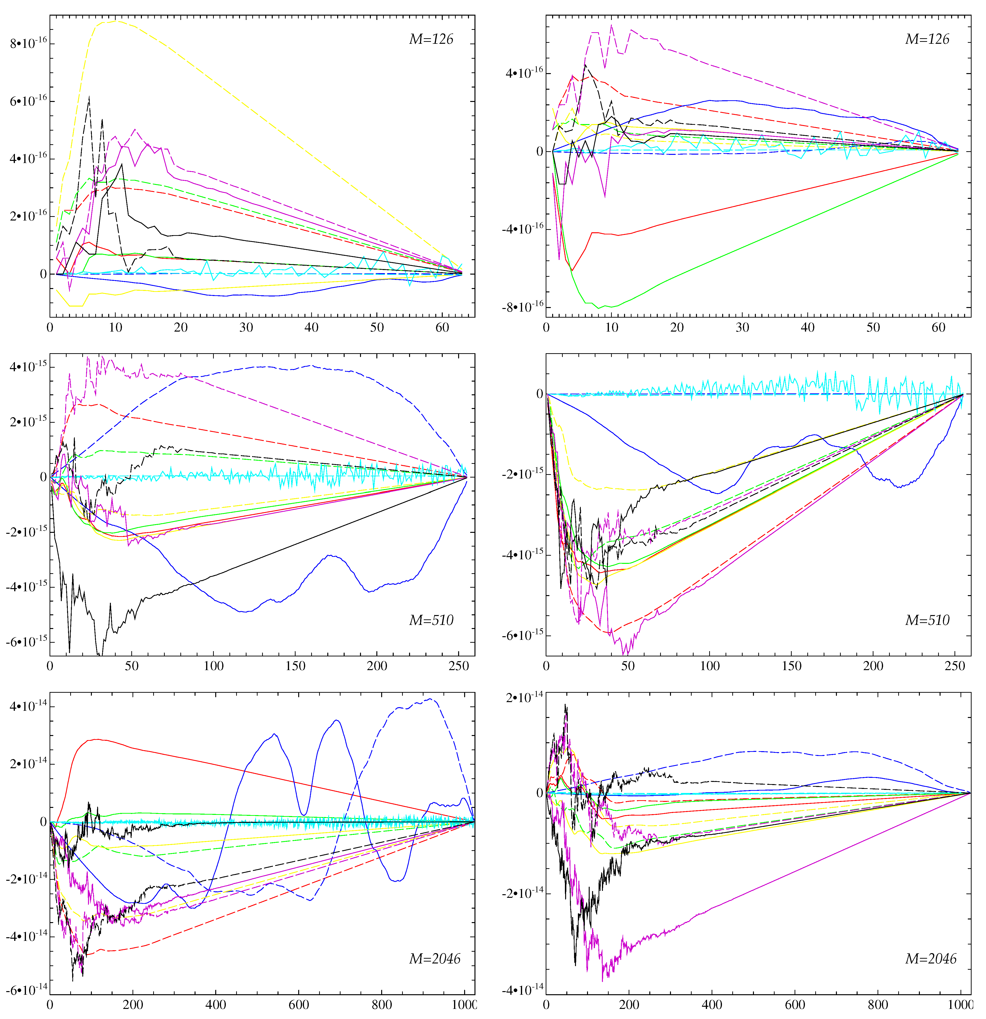
- vii.
- Solutions obtained by all algorithms except for two and three have significantly larger errors for small n (say, for ) than for larger n (see Figure 3). By contrast, algorithms 2 and 3 yield maximum errors for intermediate and high n. In addition, the errors in solutions computed by algorithm 3 wildly oscillate, which is not typical for the behaviour of errors generated by the other six algorithms. Consequently, algorithms 2 and 3 yield approximate solutions in which for intermediate and high n have exceptionally high relative errors.
- viii.
- Algorithms 2 and are significantly faster than the other five algorithms (see Table 2). Their execution CPU times are mutually close and differ much more from the execution times registered for the other ones.
3.2. Algorithms for Determining the Coefficients of a Linear Combination of
- i.
- None of the four algorithms is “perfect”: for all considered M and for both error norms, when solving the test problems each algorithm delivers solutions of any possible relative accuracy from the best to the worst one, in the sense that solutions to some test problems obtained by any algorithm have the smallest, the largest or any intermediate error norms among the four error norms produced by the four algorithms for this problem.
- ii.
- The quantities have the maxima at (see Figure 5), i.e., for each algorithm the error norms fall into the second bin, , with the highest probability.
- iii.
- For any M and for both error norms, algorithm delivers the best accuracy solutions (has the maximum over k) more often than the other three. For and 508, the least accurate solutions are obtained most frequently by algorithm and for by algorithm 2.
- iv.
- The errors for intermediate and high n (say, for ) in approximate solutions computed by algorithm are significantly larger than in solutions obtained by any of the other three algorithms.
- v.
- The execution CPU times of algorithms 1 and are slightly larger than those for algorithms 2 and .
4. Discretisation of the Magnetic Field
5. Conclusions
Author Contributions
Funding
Data Availability Statement
Conflicts of Interest
References
- Podvigina, O.M. A route to magnetic field reversals: An example of an ABC-forced non-linear dynamo. Geophys. Astrophys. Fluid Dyn. 2003, 97, 149–174. [Google Scholar] [CrossRef]
- Chertovskih, R.; Gama, S.M.A.; Podvigina, O.; Zheligovsky, V. Dependence of magnetic field generation by thermal convection on the rotation rate: A case study. Physica D 2010, 239, 1188–1209. [Google Scholar] [CrossRef]
- Jones, C.A.; Roberts, P.H. Convection-driven dynamos in a rotating plane layer. J. Fluid Mech. 2000, 404, 311–343. [Google Scholar] [CrossRef]
- Rotvig, J.; Jones, C.A. Rotating convection-driven dynamos at low Ekman number. Phys. Rev. E 2002, 66, 056308. [Google Scholar] [CrossRef]
- Eltayeb, I.A.; Rahman, M.M. Model III: Benard convection in the presence of horizontal magnetic field and rotation. Phys. Earth Planet. Inter. 2013, 221, 38–59. [Google Scholar] [CrossRef]
- Zheligovsky, V. Space analyticity and bounds for derivatives of solutions to the evolutionary equations of diffusive magnetohydrodynamics. Mathematics 2021, 9, 1789. [Google Scholar] [CrossRef]
- Stellmach, S.; Hansen, U. An efficient spectral method for the simulation of dynamos in Cartesian geometry and its implementation on massively parallel computers. Geochem. Geophys. Geosyst. 2008, 9, Q05003. [Google Scholar] [CrossRef]
- Fox, L.; Parker, I.B. Chebyshev Polynomials in Numerical Analysis; Oxford University Press: London, UK, 1968. [Google Scholar]
- Canuto, C.; Hussaini, M.Y.; Quarteroni, A.; Zang, T.A. Spectral Methods in Fluid Dynamics; Springer: Berlin/Heidelberg, Germany, 1988. [Google Scholar] [CrossRef]
- Peyret, R. Spectral Methods for Incompressible Viscous Flow; Springer: Berlin/Heidelberg, Germany, 2002. [Google Scholar] [CrossRef]
- Kleiser, L.; Schumann, U. Treatment of incompressibility and boundary conditions in 3-D numerical spectral simulations of plane channel flows. In Proceedings of the Third GAMM—Conference on Numerical Methods in Fluid Mechanics, Cologne, Germany, 10–12 October 1979; Hirschel, E.H., Ed.; Notes on Numerical Fluid Mechanics; Vieweg+Teubner Verlag: Wiesbaden, Germany, 1980; Volume 2, pp. 165–173. [Google Scholar]
- Werne, J. Incompressibility and no-slip boundaries in the Chebyshev-Tau approximation: Correction to Kleiser and Schumann’s influence-matrix solution. J. Comput. Phys. 1995, 120, 260–265. [Google Scholar] [CrossRef]
- Meseguer, Á.; Trefethen, L.N. Linearized pipe flow to Reynolds number 107. J. Comput. Phys. 2003, 186, 178–197. [Google Scholar] [CrossRef]
- O’Connor, L.; Lecoanet, D.; Anders, E.H. Marginally stable thermal equilibria of Rayleigh–Bénard convection. Phys. Rev. Fluids 2021, 6, 093501. [Google Scholar] [CrossRef]
- Reetz, F.; Schneider, T. Invariant states in inclined layer convection. Part 1. Temporal transitions along dynamical connections between invariant states. J. Fluid Mech. 2020, 898, A22. [Google Scholar] [CrossRef]
- Wen, B.; Goluskin, D.; LeDuc, M.; Chini, G.P.; Doering, C.R. Steady Rayleigh–Bénard convection between stress-free boundaries. J. Fluid Mech. 2020, 905, R4. [Google Scholar] [CrossRef]
- Wen, B.; Goluskin, D.; Doering, C.R. Steady Rayleigh–Bénard convection between no-slip boundaries. J. Fluid Mech. 2022, 933, R4. [Google Scholar] [CrossRef]
- Alboussière, T.; Drif, K.; Plunian, F. Dynamo action in sliding plates of anisotropic electrical conductivity. Phys. Rev. E 2020, 101, 033107. [Google Scholar] [CrossRef]
- Sreenivasan, B.; Gopinath, V. Confinement of rotating convection by a laterally varying magnetic field. J. Fluid Mech. 2017, 822, 590–616. [Google Scholar] [CrossRef]
- Perez-Espejel, D.; Avila, R. Linear stability analysis of the natural convection in inclined rotating parallel plates. Phys. Lett. A 2019, 383, 859–866. [Google Scholar] [CrossRef]
- Gottlieb, D.; Orszag, S.A. Numerical Analysis of Spectral Methods: Theory and Applications; SIAM-CBMS: Philadelphia, USA, 1977. [Google Scholar]
- Tuckerman, L.S. Divergence-free velocity fields in nonperiodic geometries. J. Comput. Phys. 1989, 80, 403–441. [Google Scholar] [CrossRef]
- Cox, S.M.; Matthews, P.C. Exponential time differencing for stiff systems. J. Comput. Phys. 2002, 176, 430–455. [Google Scholar] [CrossRef]
- Chertovskih, R.; Rempel, E.L.; Chimanski, E.V. Magnetic field generation by intermittent convection. Phys. Lett. A 2017, 381, 3300–3306. [Google Scholar] [CrossRef]
- Chertovskih, R.; Chimanski, E.V.; Rempel, E.L. Route to hyperchaos in Rayleigh–Bénard convection. Europhys. Lett. 2015, 112, 14001. [Google Scholar] [CrossRef]
- Jeyabalan, S.R.; Chertovskih, R.; Gama, S.; Zheligovsky, V. Nonlinear large-scale perturbations of steady thermal convective dynamo regimes in a plane layer of electrically conducting fluid rotating about the vertical axis. Mathematics 2022, 10, 2957. [Google Scholar] [CrossRef]
- Braginsky, S.I.; Roberts, P.H. Equations governing convection in Earth’s core and the geodynamo. Geophys. Astrophys. Fluid Dynamics 1995, 79, 1–97. [Google Scholar] [CrossRef]
- Boyd, J.P. Chebyshev and Fourier Spectral Methods; Dover: Downers Grove, IL, USA, 2001. [Google Scholar]
- Schmitt, B.J.; von Wahl, W. Decomposition of solenoidal fields into poloidal fields, toroidal fields and the mean flow. Applications to the Boussinesq–equations. In The Navier–Stokes Equations II—Theory and Numerical Methods. Proceedings, Oberwolfach 1991; Lecture Notes in Math; Heywood, J.G., Masuda, K., Rautmann, R., Solonnikov, S.A., Eds.; Springer: Berlin, Germany, 1992; Volume 1530, pp. 291–305. [Google Scholar] [CrossRef]
- Lanczos, C. Applied Analysis; Prentice-Hall: Englewood Cliffs, NJ, USA, 1956. [Google Scholar]
- Madabhushi, R.K.; Balachandar, S.; Vanka, S.P. A divergence-free Chebyshev collocation procedure for incompressible flows with two non-periodic directions. J. Comput. Phys. 1993, 105, 199–206. [Google Scholar] [CrossRef]
- Rivlin, T.J. Chebyshev Polynomials: From Approximation Theory to Algebra and Number Theory; Wiley-Interscience: Hoboken, NJ, USA, 1974. [Google Scholar]
- Shen, J. Efficient spectral-Galerkin method II. Direct solvers of second and fourth order equations by using Chebyshev polynomials. SIAM J. Sci. Comput. 1995, 16, 74–87. [Google Scholar] [CrossRef]
- Godunov, S.K.; Ryabenkii, V.S. Difference Schemes. An Introduction to the Underlying Theory, 1st ed.; Elsevier: Amsterdam, The Netherlands, 1987. [Google Scholar]
- Li, Z.-C.; Chien, C.-S.; Huang, H.-T. Effective condition number for finite difference method. J. Comp. Appl. Math. 2007, 198, 208–235. [Google Scholar] [CrossRef]
- Mason, J.C.; Handscomb, D.C. Chebyshev Polynomials; CRC Press: Boca Raton, FL, USA, 2003. [Google Scholar] [CrossRef]
- Il’in, V.P.; Karpov, V.V.; Maslennikov, A.M. Numerical Methods for Solving Structural Mechanics Problems. A Handbook; Vyshaishaya Shkola: Minsk, Russia, 1990. [Google Scholar]


| M | Algorithm | ||||
|---|---|---|---|---|---|
| Min. Error | Max. Error | Min. Error | Max. Error | ||
| 126 | 1 | ||||
| 2 | |||||
| 3 | |||||
| 4 | |||||
| 510 | 1 | ||||
| 2 | |||||
| 3 | |||||
| 4 | |||||
| 2046 | 1 | ||||
| 2 | |||||
| 3 | |||||
| 4 | |||||
| Algorithm | 1 | 2 | ||
|---|---|---|---|---|
| Algorithm | 3 | 4 | ||
| M | Algorithm | ||||
|---|---|---|---|---|---|
| Min. Error | Max. Error | Min. Error | Max. Error | ||
| 124 | 1 | ||||
| 2 | |||||
| 508 | 1 | ||||
| 2 | |||||
| 2044 | 1 | ||||
| 2 | |||||
| Algorithm | 1 | 2 | ||
|---|---|---|---|---|
Disclaimer/Publisher’s Note: The statements, opinions and data contained in all publications are solely those of the individual author(s) and contributor(s) and not of MDPI and/or the editor(s). MDPI and/or the editor(s) disclaim responsibility for any injury to people or property resulting from any ideas, methods, instructions or products referred to in the content. |
© 2023 by the authors. Licensee MDPI, Basel, Switzerland. This article is an open access article distributed under the terms and conditions of the Creative Commons Attribution (CC BY) license (https://creativecommons.org/licenses/by/4.0/).
Share and Cite
Tolmachev, D.; Chertovskih, R.; Zheligovsky, V. Algorithmic Aspects of Simulation of Magnetic Field Generation by Thermal Convection in a Plane Layer of Fluid. Mathematics 2023, 11, 808. https://doi.org/10.3390/math11040808
Tolmachev D, Chertovskih R, Zheligovsky V. Algorithmic Aspects of Simulation of Magnetic Field Generation by Thermal Convection in a Plane Layer of Fluid. Mathematics. 2023; 11(4):808. https://doi.org/10.3390/math11040808
Chicago/Turabian StyleTolmachev, Daniil, Roman Chertovskih, and Vladislav Zheligovsky. 2023. "Algorithmic Aspects of Simulation of Magnetic Field Generation by Thermal Convection in a Plane Layer of Fluid" Mathematics 11, no. 4: 808. https://doi.org/10.3390/math11040808
APA StyleTolmachev, D., Chertovskih, R., & Zheligovsky, V. (2023). Algorithmic Aspects of Simulation of Magnetic Field Generation by Thermal Convection in a Plane Layer of Fluid. Mathematics, 11(4), 808. https://doi.org/10.3390/math11040808