The Mixed Finite Element Reduced-Dimension Technique with Unchanged Basis Functions for Hydrodynamic Equation

Abstract

The mixed finite element (MFE) method is one of the most valid numerical approaches to solve hydrodynamic equations because it can be very suited to solving problems with complex computing domains. Regrettably, the MFE method for the hydrodynamic equations would include lots of unknowns. Especially, when it is applied to settling the practical engineering problems, it could contain hundreds of thousands and even tens of millions of unknowns. Thus, it would bring about many difficulties for actual applications, such as consuming a long CPU running time and accumulating many round-off errors, so as to be very difficult to obtain the desired numerical solutions. Therefore, we herein take the two-dimensional (2D) unsteady Navier–Stokes equation in hydrodynamics as an example. Using the proper orthogonal decomposition to lower the dimension of unknown Crank–Nicolson MFE (CNMFE) solution coefficient vectors for the 2D unsteady Navier–Stokes equation about vorticity–stream functions, we construct a reduced-dimension recursive CNMFE (RDRCNMFE) method with unchanged basis functions. In the circumstances, the RDRCNMFE method can keep the basis functions unchanged in an MFE subspace and has the same precision as the classical CNMFE method. We employ the matrix method to analyse the existence and stability along with errors to the RDRCNMFE solutions, leading to a very simple theory analysis. We use the numerical simulations for the backwards-facing step flow to verify the effectiveness of the RDRCNMFE method. The RDRCNMFE method with unchanged basis functions only reduces the dimension of the solution coefficient vectors of the CNMFE, which is completely different from previous order reduction methods which greatly affects the accuracy by reducing the dimension of the MFE subspace.

1. Introduction

Let $\Omega \subset {\mathbb{R}}^2$ be the bounded and connected domain with the boundary $\partial \Omega$. We consider the following two-dimensional (2D) incompressible nonlinear unsteady Navier–Stokes equation (see [1,2,3]).

Problem 1.

Find $\left(u\right(x,y,t),v(x,y,t\left)\right)$ and $p(x,y,t)$, satisfying

$$\begin{array}{ccc}\hfill & & {\displaystyle {\partial }_{t}u(x,y,t)-\mu \Delta u(x,y,t)+u(x,y,t){\partial }_{x}u(x,y,t)+v(x,y,t){\partial }_{y}u(x,y,t)+{\partial }_{x}p(x,y,t)}\hfill \\ \hfill {\displaystyle }& & =g_1(x,y,t),(x,y,t)\in \Omega \times (0,t_e),\hfill \\ \hfill {\displaystyle }& & {\displaystyle {\partial }_{t}v(x,y,t)-\mu \Delta v(x,y,t)+u(x,y,t){\partial }_{x}v(x,y,t)+v(x,y,t){\partial }_{y}v(x,y,t)+{\partial }_{y}p(x,y,t)}\hfill \\ \hfill {\displaystyle }& & =g_2(x,y,t),(x,y,t)\in \Omega \times (0,t_e),\hfill \\ \hfill {\displaystyle }& & {\displaystyle {\partial }_{x}u(x,y,t)+{\partial }_{y}v(x,y,t)=0,(x,y,t)\in \Omega \times (0,t_e),}\hfill \\ \hfill {\displaystyle }& & u(x,y,t)=u_0(x,y,t),v(x,y,t)=v_0(x,y,t),(x,y,t)\in \partial \Omega \times (0,t_e),\hfill \\ \hfill {\displaystyle }& & u(x,y,0)=u^0(x,y),v(x,y,0)=v^0(x,y),(x,y)\in \Omega ,\hfill \end{array}$$

where ${(u,v)}^T$ stands for the vector of fluid velocity, p stands for the pressure, ${\partial }_z=\partial /\partial z$$(z=t,$ $x,$ and $y)$, $\Delta ={\partial }^2/\partial x^2+{\partial }^2/\partial y^2$, $t_e$ stands for the last moment, $\mu =1/Re$, $Re$ is the Reynolds number, and ${(g_1(x,y,t),g_2(x,y,t))}^T$, ${(u^0(x,y),v^0(x,y))}^T$, and $(u_0(x,y,t),$$v_0{(x,y,t))}^T$ are the known source term vector, initial value vector, and boundary value vector, respectively.

The nonlinear unsteady Navier–Stokes equation is one of the most important equations in hydrodynamics and was successfully used to simulate lots of practical engineering problems (see [1,2,3]). However, on account of its nonlinearity, in particular, when its calculation domain $\Omega$ is an irregular geometrical shape, or its initial value vector, or its source term vector, or its initial value vector, or its boundary value vector is complex, we can not find its analytical solutions, so we have to find its numerical solutions.

The Crank–Nicolson (CN) mixed finite element (FE) (MFE) (CNMFE) algorithm has unconditional stability and convergence and possesses the second time precision, so it is considered to be one of the most valid methods to solve the 2D unsteady Navier–Stokes equation about the vorticity–stream functions. However, it usually contains lots of unknowns. Thereby, the primary mission of this paper is to lower the unknowns of the CNMFE algorithm so as to alleviate the computing load, save the CPU runtime, ease off the rounding errors accumulating, and acquire the desired numerical solutions.

Numerous numerical experiments (see [4,5,6,7,8,9,10,11,12,13,14]) have demonstrated that the proper orthogonal decomposition (POD) method is one of the most effective approaches to lessen the unknowns for numerical methods of the unsteady partial differential equations (PDEs). The POD method is a very old method; its predecessor is the principal vector analysis. The POD method is mainly to find a set of orthogonal bases for a given data set in a some least-squares sense, namely it is to look for the lower-dimensional optimal approximations for the set of known data. It was an eigenvector procedure technique, which was firstly addressed by Pearson in 1901 and was applied to extracting main ingredients in massive data (see [15]). Pearson’s data mining is used at present. The fashionable name for such processed data is just the so-called “Big Data”. The method for snapshots of the POD was first proposed by Sirovich in 1987 (see [16]).

Based on the effectiveness with which the POD method deals with data, the POD method has been broadly and resoundingly applied in various fields, such as atmospheric sciences and hydrodynamics (see [17]), image recognition and signal procedures (see [18]), together with statistics (see [19]). However, for a long time, since 1987, the POD method was mainly applied to implementing the main vector analysis in statistics and researching the main behaviour in hydrodynamics. It was not until 2001 that the POD method was used by Kunisch and Volkweind to construct the Galerkin reduced-order methods for PDEs (see [1,20]). From that time on, the model order reduction and reduced basis for the numerical methods based on the POD for PDEs was rapidly developed and produced a significant efficiency for solving unsteady PDEs (see [4,5,6,7,8,9,11,12,13,14]). However, these model order reduction and reduced basis methods are mainly to lower the dimensionality of the FE subspaces, namely that the FE subspaces are replaced with the subspace generated by POD basis functions, resulting in the accuracy of the model order reduction and reduced basis methods being greatly influenced by the POD reduced order. In this paper, we adopt the POD method to reduce the dimensionality of the unknown solution coefficient vectors for the CNMFE method of the unsteady Navier–Stokes equation about the vorticity–stream functions and to construct the reduced-dimension recursive CNMFE (RDRCNMFE) method, which is completely different from the order reduction methods about FE subspaces above, including the reduced-order method in [10]. In this case, we only lower the dimension of unknown CNMFE solution coefficient vectors so as to ensure that the basis functions and precision of the RDRCNMFE method are the same as the CNMFE one but with few unknowns.

Though the reduced-dimension models for the unknown coefficient vectors of FE solutions of the parabolic equation, hyperbolic equation, Sobolev equation, unsteady Stokes equation, and Rosenau equation were, respectively, established in [21,22,23,24,25], the non-stationary Navier–Stokes equation is far more complex than the five types of equations in [21,22,23,24,25] because it not only includes the pressure but also contains the fluid velocity vector and is nonlinear. Thereby, either the creation of the RDRCNMFE model or the theory analysis for the existence and stability as well as errors of the RDRCNMFE solutions would face more difficulties and need more skills than those in [21,22,23,24,25]. However, the RDRCNMFE method for the unsteady Navier–Stokes equation has very important applications. So, it is of great value to study the RDRCNMFE method of the unsteady Navier–Stokes equation.

For this purpose, we first construct the CNMFE method with the second-order time precision, and the unconditional stability and convergence for the 2D unsteady Navier–Stokes equation for the vorticity–stream functions, and discuss the existence and stability as well as convergence for the CNMFE solutions in Section 2. In addition, in Section 3, we employ the POD method to construct the POD basis vectors and establish the RDRCNMFE method, and we adopt the matrix analysis to discuss the existence, stability, and convergence of the RDRCNMFE solutions. Afterwards, in Section 4, we utilise some numerical simulations to reveal the effectiveness and feasibility of the RDRCNMFE method and validate that the numerical calculating results are accorded with the theoretical results. Finally, we epitomise the main conclusions in Section 5.

2. The CNMFE Method for the Unsteady Navier–Stokes Equation

The Sobolev spaces and norms used herein are standard (see [26]). For convenience’s sake, we suppose that ${(u_0,v_0)}^T=\mathbf{0}$ and $\mathbb{U}=H_0^1(\Omega )$ in the follow-up theories analysis.

2.1. The Time Semi-Discretised CN Scheme

On account of boundedness of the domain $\Omega$, the equation ${\displaystyle {\partial }_{x}u+{\partial }_{y}v=0}$ has a unique stream function $\psi$ satisfying ${\displaystyle u={\partial }_y\psi }$ and $v=-{\partial }_x\psi .$ Moreover, there exists a vorticity function $\varpi$, satisfying ${\displaystyle \varpi ={\partial }_{x}v-{\partial }_{y}u=-\Delta \psi }$. Therewith, Problem 1 may be converted into the following system of equations in regard to the vorticity–stream functions $(\psi ,\varpi )$.

Problem 2.

Find $(\psi ,\varpi )$, satisfying

$$\begin{array}{ccc}\hfill & & \left\{\begin{array}{cc}{\displaystyle -\Delta \psi (x,y,t)=\varpi (x,y,t),}\hfill & (x,y,t)\in \Omega \times (0,t_e),\hfill \\ {\displaystyle \psi (x,y,t)=0,}\hfill & (x,y,t)\in \partial \Omega \times (0,t_e),\hfill \end{array}\right.\hfill \end{array}$$

(1)

$$\begin{array}{ccc}\hfill & & \left\{\begin{array}{c}{\displaystyle {\partial }_t\varpi (x,y,t)-\mu \Delta \varpi (x,y,t)+{\partial }_y\psi (x,y,t){\partial }_x\varpi (x,y,t)-{\partial }_x\psi (x,y,t){\partial }_y\varpi (x,y,t)}\hfill \\ {\displaystyle =f(x,y,t),(x,y,t)\in \Omega \times (0,t_e),}\hfill \\ {\displaystyle \varpi (x,y,t)=0,(x,y,t)\in \partial \Omega \times (0,t_e),}\hfill \\ {\displaystyle \varpi (x,y,0)={\varpi }^0(x,y),(x,y)\in \Omega ,}\hfill \end{array}\right.\hfill \end{array}$$

(2)

where $f={\partial }_x{g}_2-{\partial }_y{g}_1$ and ${\varpi }^0(x,y)={\partial }_x{v}^0(x,y)-{\partial }_y{u}^0(x,y)$.

Let $N>0$ represent the integer, let $\Delta t=t_e/N$ stand for the time step, and let ${\varpi }^n(x,y)$ and ${\psi }^n(x,y)$ be, respectively, the approximations to $\varpi (t,x,y)$ and $\psi (x,y,t)$ at $t_n=n\Delta t$. By using the CN method to discretise the first derivative of time in (2), the time semi-discretised CN scheme with the second-order accuracy in time may be expressed in the following.

Problem 3.

Find $({\varpi }^n,{\psi }^n)\in \mathbb{U}\times \mathbb{U}$$(1⩽n⩽N)$, satisfying

$$\begin{array}{ccc}& & {\displaystyle a({\psi }^{n-1},w)=({\varpi }^{n-1},w),\forall w\in \mathbb{U},1⩽n⩽N+1;}\hfill \\ & & {\displaystyle ({\varpi }^n,w)+0.5\mu \Delta ta({\varpi }^n,w)=({\varpi }^{n-1},w)-0.5\mu \Delta ta({\varpi }^{n-1},w)+(f^{n-\frac{1}{2}},w)}\hfill \\ \hfill & & {\displaystyle +\Delta t{a}_1({\psi }^{n-1},{\varpi }^{n-1},w),\forall w\in \mathbb{U},1⩽n⩽N,}\hfill \end{array}$$

where $a(\psi ,\varpi )=(\nabla \psi ,\nabla \varpi )$, $(·,·)$ is the $L^2$ inner product, $f^{n-\frac{1}{2}}=(x,y,t_{n-\frac{1}{2}})$, and ${\displaystyle a_1(\psi ,\varpi ,\varphi )}$${\displaystyle ={\int }_{\Omega }\left({\partial }_x\psi {\partial }_y\varpi -{\partial }_y\psi {\partial }_x\varpi \right)\varphi \mathrm{d}x\mathrm{d}y}$.

The following properties of ${\displaystyle a_1(\psi ,\varpi ,\varphi )}$ are known (see [3]).

$$\begin{array}{c}\hfill \left\{\begin{array}{c}{\displaystyle a_1(\psi ,\varpi ,\varphi )=-a_1(\psi ,\varphi ,\varpi ),\forall \psi ,\varpi ,\varphi \in H_0^1(\Omega );}\hfill \\ {\displaystyle a_1(\psi ,\varpi ,\varpi )=0\forall \psi ,\varpi \in H_0^1(\Omega );}\hfill \\ {\displaystyle |a_1{(\psi ,\varpi ,\varphi )|⩽c\parallel \nabla \left(\mathrm{curl}\psi \right)\parallel }_0{\parallel \nabla \varpi \parallel }_0{\parallel \nabla \varphi \parallel }_0,\forall \psi ,\varpi ,\varphi \in H_0^1(\Omega ).}\hfill \end{array}\right.\end{array}$$

(3)

When ${\varpi }^{(n-1)}\in L^{\infty }(\Omega )$ and $f^{n-\frac{1}{2}}\in L^{\infty }(\Omega )$ are given, it is obvious that Problem 3 is two relatively independent variational problems of standard elliptic equations about the unknowns ${\psi }^{n-1}$ and ${\varpi }^n$, so that there exists a unique set of solutions ${\left\{({\varpi }^n,{\psi }^n)\right\}}_{n=1}^N\subset \mathbb{U}\times \mathbb{U}$ satisfying the following unconditional stability:

$$\begin{array}{ccc}\hfill {\displaystyle }& & \parallel {\psi }^n{\parallel }_{1,\infty }+{\parallel {\varpi }^n\parallel }_{0,\infty }⩽c,1⩽n⩽N,\hfill \end{array}$$

(4)

where c used a follow-up that is a general positive constant that is only dependent on ${\varpi }^0$, f, $Re$, and $t_e$ and is different in different places. Moreover, using Taylor’s formula, we can easily conclude that the set of solutions ${\displaystyle {\left\{({\varpi }^n,{\psi }^n)\right\}}_{n=1}^N}$⊂$\mathbb{U}\times \mathbb{U}$ has the second-order time accuracy, namely that

$$\begin{array}{ccc}\hfill {\displaystyle }& & \parallel \psi \left(t_n\right)-{\psi }^n{\parallel }_{1,\infty }+{\parallel \varpi \left(t_n\right)-{\varpi }^n\parallel }_{0,\infty }⩽c\Delta t^2,\hfill \end{array}$$

(5)

where $(\varpi \left(t_n\right),\psi \left(t_n\right))$ are the state of solution $(\varpi ,\psi )$ for Problem 2 at $t=t_n$ ($1⩽n⩽N$).

2.2. The Fully Discretised CNMFE Method

Let ${\Im }_h$ be a regular triangulation on $\overline{\Omega }$ and the M-dimensional FE space ${\mathbb{U}}_h$, generated by the orthonormal bases ${\left\{{\zeta }_j\left(\mathit{x}\right)\right\}}_{j=1}^M$ under the inner product in $L^2(\Omega )$ (where ${\zeta }_j\left(\mathit{x}\right)$ are obtained by the standard orthogonalisation in Section 6.3 [26]), be denoted by

$$\begin{array}{lll}{\displaystyle {\mathbb{U}}_h}& =& {\displaystyle \left\{{\upsilon }_h\in H_0^1(\Omega )\cap C(\Omega ):{\upsilon }_h{|}_K\in {\mathbb{P}}_l\left(K\right),K\in {\Im }_h\right\}}\\ & =& {\displaystyle \mathrm{span}\left\{{\zeta }_j\left(\mathit{x}\right):1⩽j⩽M\right\},}\end{array}$$

(6)

where ${\mathbb{P}}_l\left(K\right)$ is formed with lth degree polynomials on $K\in {\Im }_h$. Thus, the CNMFE format may be expressed in the following.

Problem 4.

Find ${\left\{({\varpi }_h^n,{\psi }_h^n)\right\}}_{n=1}^N\subset {\mathbb{U}}_h\times {\mathbb{U}}_h$, satisfying

$$\begin{array}{ccc}\hfill & & {\displaystyle a({\psi }_h^{n-1},w_h)=({\varpi }_h^{n-1},w_h),\forall w_h\in {\mathbb{U}}_h,1⩽n⩽N+1;}\hfill \end{array}$$

(7)

$$\begin{array}{ccc}& & {\displaystyle ({\varpi }_h^n,w_h)+0.5\mu \Delta ta({\varpi }_h^n,w_h)=({\varpi }_h^{n-1},w_h)-0.5\mu \Delta ta({\varpi }_h^{n-1},w_h)}\hfill \\ \hfill & & {\displaystyle +\Delta t{a}_1({\psi }_h^{n-1},{\varpi }_h^{n-1},w_h)+(f^{n-\frac{1}{2}},w_h),\forall w_h\in {\mathbb{U}}_h,1⩽n⩽N,}\hfill \end{array}$$

(8)

where ${\varpi }_h^0=R_h{\varpi }^0$ and $R_h$ is Ritz-Projection, namely meets the following equation

$$\begin{array}{ccc}& & (\nabla R_h{\varpi }^0,\nabla {\upsilon }_h)=(\nabla {\varpi }^0,\nabla {\upsilon }_h),\forall {\upsilon }_h\in {\mathbb{U}}_h.\hfill \end{array}$$

Noting that (7) and (8) in Problem 4 for the known ${\varpi }_h^{n-1}$ and ${\psi }_h^{n-1}$ constitutes the standard system of elliptic problems, by standard FE method and the Lax–Milgram theorem, we can easily prove the following existence, stability, and convergence about the CNMFE solution of Problem 4.

Theorem 1.

Problem 4 has a unique set of solutions ${\left\{({\varpi }_h^n,{\psi }_h^n)\right\}}_{n=1}^N\subset {\mathbb{U}}_h\times {\mathbb{U}}_h$ satisfying the following unconditional stability:

$$\begin{array}{ccc}\hfill {\displaystyle }& & \parallel {\psi }_h^n{\parallel }_{1,\infty }+{\parallel {\varpi }_h^n\parallel }_{0,\infty }⩽c,1⩽n⩽N,\hfill \end{array}$$

(9)

and error estimates

$$\begin{array}{ccc}\hfill {\displaystyle }& & \parallel \varpi \left(t_n\right)-{\varpi }_h^n{\parallel }_{0,\infty }⩽c(\Delta t^2+h^{l+1}),1⩽n⩽N,\hfill \end{array}$$

(10)

$$\begin{array}{ccc}\hfill {\displaystyle }& & {\displaystyle \parallel \psi \left(t_n\right)-{\psi }_h^n{\parallel }_{1,\infty }⩽c(\Delta t^2+h^l),1⩽n⩽N,}\hfill \end{array}$$

(11)

where $(\varpi \left(t_n\right),\psi \left(t_n\right))$ are the state of solution $(\varpi ,\psi )\in {[W^{l+1,\infty }(\Omega )\cap H_0^1(\Omega )]}^2$ of Problem 2 at $t=t_n$$(1⩽n⩽N)$.

Let ${\mathbf{\varpi }}^n={({\varpi }_1^n,{\varpi }_2^n,\cdots ,{\varpi }_M^n)}^T,$${\mathbf{\psi }}^n=({\psi }_1^n,{\psi }_2^n,\cdots ,$${\psi }_M^n{)}^T,$ and $\mathbf{\zeta }=({\zeta }_1,{\zeta }_2,\cdots ,$${\zeta }_M{)}^T$. Then, the solutions $({\varpi }_h^n,{\psi }_h^n)$ for Problem 4 may be denoted by

$$\begin{array}{ccc}& & {\varpi }_h^n=\sum _{j=1}^M{\varpi }_j^n{\zeta }_j=\mathbf{\zeta }·{\mathbf{\varpi }}^n,{\psi }_h^n=\sum _{j=1}^M{\psi }_j^n{\zeta }_j=\mathbf{\zeta }·{\mathbf{\psi }}^n.\hfill \end{array}$$

Thus, Problem 4 may be written into the following matrix format.

Problem 5.

Find $({\mathbf{\varpi }}^n,{\mathbf{\psi }}^n)\in {\mathbb{R}}^M\times {\mathbb{R}}^M$ and $({\varpi }_h^n,{\psi }_h^n)\in {\mathbb{U}}_h\times {\mathbb{U}}_h$$(1⩽n⩽N)$, satisfying

$$\begin{array}{ccc}\hfill & & {\displaystyle \mathit{B}{\mathbf{\psi }}^{n-1}={\mathbf{\varpi }}^{n-1},1⩽n⩽N+1;}\hfill \\ & & {\displaystyle \left(\mathit{I}+0.5\mu \Delta t\mathit{B}\right){\mathbf{\varpi }}^n=\left(\mathit{I}-0.5\mu \Delta t\mathit{B}\right){\mathbf{\varpi }}^{n-1}}\hfill \end{array}$$

(12)

$$\begin{array}{ccc}\hfill & & {\displaystyle +\Delta t\widehat{\mathit{B}}\left({\psi }_h^{n-1}\right){\mathbf{\varpi }}^{n-1}+\Delta t{\mathit{F}}^n,1⩽n⩽N,}\hfill \end{array}$$

(13)

$$\begin{array}{ccc}\hfill & & {\displaystyle {\varpi }_h^n=\mathbf{\zeta }·{\mathbf{\varpi }}^n,{\psi }_h^n=\mathbf{\zeta }·{\mathbf{\psi }}^n,1⩽n⩽N,}\hfill \end{array}$$

(14)

where $\mathit{B}={\left(a({\zeta }_i,{\zeta }_j)\right)}_{M\times M}$, $\widehat{\mathit{B}}\left({\psi }_h^{n-1}\right)$$={(({\partial }_x{\psi }_h^{n-1}{\partial }_y{\zeta }_i,{\zeta }_j)-({\partial }_y{\psi }_h^{n-1}{\partial }_x{\zeta }_i,{\zeta }_j))}_{M\times M}$, $\mathit{I}$ is the $M\times M$ identity matrix, ${\mathit{F}}^n={((f^{n-\frac{1}{2}},{\zeta }_1),(f^{n-\frac{1}{2}},{\zeta }_2),\cdots ,(f^{n-\frac{1}{2}},{\zeta }_M))}^T$, and $(·,·)$ is the $L^2$ inner product.

Remark 1.

When the spatial mesh parameter h, the time step $\Delta t$, ${(g_1,g_2)}^T$, ${(u^0,v^0)}^T$, and Reynolds $Re$ are appointed, two sets of the coefficient vectors ${\left\{{\mathbf{\psi }}^n\right\}}_{n=1}^N$ and ${\left\{{\mathbf{\varpi }}^n\right\}}_{n=1}^N$ may be obtained by Problem 5. Therewith, the velocity CNMFE solutions $(u_h^n,v_h^n)$ ($n=1,2,\cdots ,N$) may be obtained with $u_h^n=\partial {\psi }_h^n/\partial y$ and $v_h^n=-\partial {\psi }_h^n/\partial x$. Generally, the dimension of the unknown solution coefficient vectors ${\left\{{\mathbf{\psi }}^n\right\}}_{n=1}^N$ and ${\left\{{\mathbf{\varpi }}^n\right\}}_{n=1}^N$ for Problem 5 is so high that we have to lower their dimension by the POD method.

3. The RDRCNMFE Method for the Unsteady Navier–Stokes Equation

3.1. The Construction of POD Basis Vectors

We first find L coefficient vectors ${\mathbf{\varpi }}^n$ ($n=1,2,\cdots ,$L) of Problem 5 at the first L time steps and compose into an $M\times L$ snapshot matrices $\mathit{A}=({\mathbf{\varpi }}^1,{\mathbf{\varpi }}^2,\cdots ,$${\mathbf{\varpi }}^L)$. We then find the orthonormal eigenmatrix $\tilde{\mathsf{\Phi }}=({\mathbf{\phi }}_1,{\mathbf{\phi }}_2,\cdots ,$${\mathbf{\phi }}_r)\in {\mathbb{R}}^{M\times r}$$(r=$ rank$\left(\mathit{A}\right))$ of $\mathit{A}{\mathit{A}}^T$ corresponding to the positive eigenvalues ${\lambda }_1⩾{\lambda }_2⩾\cdots ⩾{\lambda }_r>0$. We may lastly obtain a set of POD bases $\mathsf{\Phi }=({\mathbf{\phi }}_1,{\mathbf{\phi }}_2,\cdots ,$${\mathbf{\phi }}_d)$ ($d⩽r$) from the initial d vectors in $\tilde{\mathsf{\Phi }}$, satisfying the following property:

$$\begin{array}{ccc}\hfill {\displaystyle }& & \parallel \mathit{A}-\mathsf{\Phi }{\mathsf{\Phi }}^T{\mathit{A}\parallel }_2=\sqrt{{\lambda }_{i,d+1}},\hfill \end{array}$$

(15)

herein ${\parallel \mathit{A}\parallel }_2={sup}_{\mathbf{\chi }\in {\mathbb{R}}^L}\parallel \mathit{A}\mathbf{\chi }\parallel /\parallel \mathbf{\chi }\parallel$ and $\parallel \mathbf{\chi }\parallel$ is the Euclidian norm of vector $\mathbf{\chi }$. Moreover, there holds the following estimates:

$$\begin{array}{l}{\displaystyle \parallel {\mathbf{\varpi }}^n-\mathsf{\Phi }{\mathsf{\Phi }}^T{\mathbf{\varpi }}^n\parallel =\parallel ({\mathit{A}}_1-\mathsf{\Phi }{\mathsf{\Phi }}^T{\mathit{A}}_1){\ell }^n\parallel ⩽\parallel {\mathit{A}}_1-\mathsf{\Phi }{\mathsf{\Phi }}^T{\mathit{A}}_1{\parallel }_2\parallel {\ell }^n\parallel }\\ {\displaystyle ⩽\sqrt{{\lambda }_{d+1}},n=1,2,\cdots ,L,}\end{array}$$

(16)

where ${\ell }^n$$(n=1,2,\cdots ,L)$ are the unit vectors whose nth element equals 1. Hence, $\mathsf{\Phi }=({\mathbf{\phi }}_1,{\mathbf{\phi }}_2,\cdots ,$${\mathbf{\phi }}_d)$ is a set of optimal POD bases.

Remark 2.

On account that the order of the $M\times M$ matrix $\mathit{A}{\mathit{A}}^T$ is greatly larger than the order of the $L\times L$ matrix ${\mathit{A}}^T\mathit{A}$, namely that the number M of nodes in ${\Im }_N$ is greatly larger than the number L of snapshots, whereas the positive eigenvalues of both ${\mathit{A}}^T\mathit{A}$ and $\mathit{A}{\mathit{A}}^T$ are the same, we may first compute out the eigenvalues ${\lambda }_j$$(j=1,2,\cdots ,r)$ of ${\mathit{A}}^T\mathit{A}$ and the relative eigenvectors ${\mathbf{\varphi }}_j$$(j=1,2,\cdots ,r)$, and then, by the formulas ${\mathbf{\phi }}_j=\mathit{A}{\mathbf{\varphi }}_j/\sqrt{{\lambda }_j}$$(j=1,2,\cdots ,r)$, we can easily obtain the eigenvectors ${\mathbf{\phi }}_j$$(j=1,2,\cdots ,r)$ corresponding to the positive eigenvalues ${\lambda }_j$$(j=1,2,\cdots ,r)$ of $\mathit{A}{\mathit{A}}^T$ to make up a set of POD bases $\mathsf{\Phi }=({\mathbf{\phi }}_1,{\mathbf{\phi }}_2,\cdots ,$${\mathbf{\phi }}_d)$ ($d⩽r$).

3.2. The Establishment of RDRCNMFE Model

If we suppose that ${\mathbf{\varpi }}_d^n={({\varpi }_{d1}^n,{\varpi }_{d2}^n,\cdots ,{\varpi }_{dM}^n)}^T$ and ${\mathbf{\beta }}^n=({\beta }_1^n,$${\beta }_2^n,\cdots ,$${\beta }_d^n{)}^T$, we can directly obtain the first $L(L⩽N)$ coefficient vectors ${\mathbf{\varpi }}_d^n$$=\mathsf{\Phi }{\mathsf{\Phi }}^T{\mathbf{\varpi }}^n=:\mathsf{\Phi }{\mathbf{\beta }}^n$ and ${\mathbf{\psi }}_d^n={\mathit{B}}^{-1}{\mathbf{\varpi }}_d^n$ $(n=1,2,\cdots ,L)$ of the RDRCNMFE solutions. Replacing the coefficient vector ${\mathbf{\varpi }}^n$ in Problem 5 with ${\mathbf{\varpi }}_d^n=\mathsf{\Phi }{\mathbf{\beta }}^n$$(n=L+1,L+2,\cdots ,N)$, by the invertibility of $(\mathit{I}+0.5\mu \Delta t\mathit{B})$, we may set up the RDRCNMFE model in the following.

Problem 6.

Find $({\mathbf{\varpi }}_d^n,{\mathbf{\psi }}_d^n)\in {\mathbb{R}}^M\times {\mathbb{R}}^M$ and $({\varpi }_d^n,{\psi }_d^n)\in {\mathbb{U}}_h\times {\mathbb{U}}_h$$(1⩽n⩽N)$, satisfying

$$\begin{array}{ccc}\hfill & & {\displaystyle {\mathbf{\beta }}^n={\mathsf{\Phi }}^T{\mathbf{\varpi }}^n,{\mathbf{\psi }}_d^n={\mathit{B}}^{-1}\mathsf{\Phi }{\mathbf{\beta }}^n,{\psi }_d^n={\mathbf{\psi }}_d^n·\mathbf{\zeta },{\mathbf{\varpi }}_d^n=\mathsf{\Phi }{\mathbf{\beta }}^n,1⩽n⩽L;}\hfill \\ \hfill & & {\displaystyle {\mathbf{\beta }}^n={\mathsf{\Phi }}^T{\left(\mathit{I}+0.5\mu \Delta t\mathit{B}\right)}^{-1}\left(\mathit{I}-0.5\mu \Delta t\mathit{B}\right)\mathsf{\Phi }{\mathbf{\beta }}^{n-1}}\hfill \\ \hfill & & {\displaystyle +\Delta t{\mathsf{\Phi }}^T{\left(\mathit{I}+0.5\mu \Delta t\mathit{B}\right)}^{-1}\widehat{\mathit{B}}\left({\psi }_d^{n-1}\right)\mathsf{\Phi }{\mathbf{\beta }}^{n-1}}\hfill \\ \hfill & & {\displaystyle +\Delta t{\mathsf{\Phi }}^T{\left(\mathit{I}+0.5\mu \Delta t\mathit{B}\right)}^{-1}{\mathit{F}}^n,L+1⩽n⩽N;}\hfill \\ \hfill & & {\displaystyle {\mathbf{\psi }}_d^n={\mathit{B}}^{-1}\mathsf{\Phi }{\mathbf{\beta }}^n,{\mathbf{\varpi }}_d^n=\mathsf{\Phi }{\mathbf{\beta }}^n,{\varpi }_d^n=\mathbf{\zeta }·{\mathbf{\varpi }}_d^n,{\psi }_d^n=\mathbf{\zeta }·{\mathbf{\psi }}_d^n,L+1⩽n⩽N;}\hfill \end{array}$$

where ${\mathbf{\varpi }}^n$ $(n=1,2,\cdots ,L)$ are the initial L solution vectors in Problem 5, and the matrices $\mathit{B}$ and $\widehat{\mathit{B}}$ are provided in Problem 5.

Remark 3.

Comparing Problem 6 with Problem 5, we can see that the CNMFE method (Problem 5) at each time step has M unknowns, while the RDRCNMFE method (Problem 6) at the same time step has only d unknowns $(d\ll M)$, but they have the same basic function ${\left\{{\zeta }_j\left(\mathit{x}\right)\right\}}_{j=1}^M$ so that the RDRCNMFE method has the same accuracy as the classical CNMFE under the case that $\sqrt{{\lambda }_{d+1}}$ is sufficiently small, namely that, although the dimension of Problem 6 is greatly lowered, the accuracy of RDRCNMFE solutions remains unchanged. So, the RDRCNMFE method (Problem 6) is overtly superior over the CNMFE method (Problem 5). After ${\psi }_d^n$ ($n=1,2,\cdots ,N$) are found by Problem 6, the RDRCNMFE solutions ${(u_d^n,v_d^n)}^T$ of the velocity can be obtained by $u_d^n={\partial }_y{\psi }_d^n$ and $v_d^n=-{\partial }_x{\psi }_d^n$. It is obvious that Problem 6 has a unique set of ${\psi }_d^n$ ($n=1,2,\cdots ,M$) so that the RDRCNMFE solutions ${(u_d^n,v_d^n)}^T$ of the velocity also uniquely exist.

3.3. The Stability and Convergence of the RDRCNMFE Solutions

To discuss the stability and convergence of the RDRCNMFE solutions needs the following two lemmas. The following lemma may be obtained from Lemmas 1.4.1 and 1.4.2 in [27].

Lemma 1.

If the $M\times M$ matrix $\mathit{B}$ is positive semi-definite, $\mathit{I}$ is the $M\times M$ identity matrix, and the real $\sigma ⩾0$, then there holds the following estimates

$$\begin{array}{ccc}& & {\parallel (\mathit{I}+\sigma \mathit{B})}^{-1}{\parallel }_2⩽1;{\parallel {(\mathit{I}+\sigma \mathit{B})}^{-1}(\mathit{I}-\sigma \mathit{B})\parallel }_2⩽1.\hfill \end{array}$$

Using the matrix norm and Lemma 1.22 in [26], we may directly obtain the following lemma.

Lemma 2.

If $(·,·)$ is the $L^2$ inner product, ${\zeta }_i$$(i=1,2,\cdots ,M)$ are the FE basis functions, and $\mathit{B}$ consists of $(\nabla {\zeta }_i,\nabla {\zeta }_j)$, then there holds the following estimates

$$\begin{array}{ccc}& & {\displaystyle {\parallel \mathit{B}\parallel }_2⩽c,{\parallel {\mathit{B}}^{-1}\parallel }_2⩽c.}\hfill \end{array}$$

Especially, if $\mathit{B}$ consists of $({\zeta }_i,{\zeta }_j)$, then there holds ${\displaystyle {\parallel \mathit{B}\parallel }_2⩽ch}$ and ${\displaystyle \parallel {\mathit{B}}^{-1}{\parallel }_2⩽c{h}^{-1}}$.

For the RDRCNMFE solutions, we have the following result of stability and convergence.

Theorem 2.

If ${\varpi }^0={\partial }_x{v}^0-{\partial }_y{u}^0\in L^{\infty }(\Omega )$, namely that $(u^0,v^0)\in W^{1,\infty }{(\Omega )}^2$, then Problem 6 has a unique set of solutions ${\left\{({\varpi }_d^n,{\psi }_d^n\right\}}_{n=1}^N$ satisfying the following stability:

$$\begin{array}{ccc}\hfill & & {\displaystyle \parallel {\varpi }_d^n{\parallel }_{0,\infty }+{\parallel {\psi }_d^n\parallel }_{1,\infty }⩽c,1⩽n⩽N.}\hfill \end{array}$$

(17)

In addition, when $(\varpi ,\psi )\in [W^{l+1,\infty }(\Omega )\cap H_0^1(\Omega )]\times [W^{l+1,\infty }(\Omega )\cap H_0^1(\Omega )]$$\cap H_0^1(\Omega )]$, there holds the following error estimates

$$\begin{array}{ccc}\hfill & & {\displaystyle \parallel \varpi \left(t_n\right)-{\varpi }_d^n{\parallel }_{0,\infty }⩽c\left(\Delta t^2+h^{l+1}+\sqrt{{\lambda }_{d+1}}\right),1⩽n⩽N,}\hfill \end{array}$$

(18)

$$\begin{array}{ccc}\hfill & & {\displaystyle \parallel \psi \left(t_n\right)-{\psi }_d^n{\parallel }_{1,\infty }⩽c\left(\Delta t^2+h^l+\sqrt{{\lambda }_{d+1}}\right),1⩽n⩽N,}\hfill \end{array}$$

(19)

where $(\varpi \left(t_n\right),\psi \left(t_n\right))$ are the state of solution $(\varpi ,\psi )$ to Problem 2 at $t=t_n$ $(n=1,2,\cdots ,N)$.

Proof. 

(1) Prove the existence of solutions to Problem 6.

It follows from Problem 6 and Remark 3 that the RDRCNMFE solutions $({\varpi }_d^n,{\psi }_d^n)$ and $(u_d^n,v_d^n)$ ($n=1,2,\cdots ,N$) are uniquely existing.

(2) Analyse the stability of solutions to Problem 6.

Using ${\mathbf{\varpi }}_d^n=\mathsf{\Phi }{\mathbf{\beta }}^n$, we may rewrite Problem 6 into the following system of equations:

$$\begin{array}{ccc}\hfill & & {\displaystyle {\mathbf{\varpi }}_d^n=\mathsf{\Phi }{\mathsf{\Phi }}^T{\mathbf{\varpi }}^n,{\mathbf{\psi }}_d^n={\mathit{B}}^{-1}{\mathbf{\varpi }}_d^n,{\varpi }_d={\mathbf{\varpi }}_d^n·\mathbf{\zeta },{\psi }_d^n={\mathbf{\psi }}_d^n·\mathbf{\zeta },1⩽n⩽L;}\hfill \end{array}$$

(20)

$$\begin{array}{ccc}\hfill & & {\displaystyle {\mathbf{\varpi }}_d^n={\left(\mathit{I}+0.5\mu \Delta t\mathit{B}\right)}^{-1}\left(\mathit{I}-0.5\mu \Delta t\mathit{B}\right){\mathbf{\varpi }}_d^{n-1}}\hfill \\ \hfill & & {\displaystyle +\Delta t{\left(\mathit{I}+0.5\mu \Delta t\mathit{B}\right)}^{-1}\widehat{\mathit{B}}\left({\psi }_d^{n-1}\right){\mathbf{\varpi }}_d^{n-1}}\hfill \\ \hfill & & {\displaystyle +\Delta t{\left(\mathit{I}+0.5\mu \Delta t\mathit{B}\right)}^{-1}{\mathit{F}}^n,L+1⩽n⩽N;}\hfill \end{array}$$

(21)

$$\begin{array}{ccc}\hfill & & {\displaystyle {\mathbf{\psi }}_d^n={\mathit{B}}^{-1}\mathsf{\Phi }{\mathbf{\beta }}^n,{\mathbf{\varpi }}_d^n=\mathsf{\Phi }{\mathbf{\beta }}^n,{\varpi }_d^n=\mathbf{\zeta }·{\mathbf{\varpi }}_d^n,{\psi }_d^n=\mathbf{\zeta }·{\mathbf{\psi }}_d^n,L+1⩽n⩽N.}\hfill \end{array}$$

(22)

When $1⩽n⩽L$, noting that $\parallel \mathsf{\Phi }{\mathsf{\Phi }}^T{\parallel }_2⩽c$, by Lemma 2 and (9) in Theorem 1, we obtain

$$\begin{array}{ccc}\hfill & & {\displaystyle \parallel {\varpi }_d^n{\parallel }_{0,\infty }=\parallel {\mathbf{\varpi }}_d^n{·\mathbf{\zeta }\parallel }_{0,\infty }={\parallel \mathsf{\Phi }{\mathsf{\Phi }}^T{\mathbf{\varpi }}^n·\mathbf{\zeta }\parallel }_{0,\infty }}\hfill \\ \hfill & & {\displaystyle ⩽\parallel \mathsf{\Phi }{\mathsf{\Phi }}^T{\parallel }_2\parallel {\mathbf{\varpi }}^n{·\mathbf{\zeta }\parallel }_{0,\infty }⩽\parallel \mathsf{\Phi }{\mathsf{\Phi }}^T{\parallel }_2{\parallel {\varpi }_h^n\parallel }_{0,\infty }⩽c;}\hfill \end{array}$$

(23)

$$\begin{array}{ccc}\hfill & & {\displaystyle \parallel {\psi }_d^n{\parallel }_{1,\infty }⩽c{\parallel {\varpi }_d^n\parallel }_{0,\infty }⩽c.}\hfill \end{array}$$

(24)

When $L+1⩽n⩽N$, using Lemmas 1 and 2, from (21), we obtain

$$\begin{array}{ccc}\hfill & & {\displaystyle \parallel {\varpi }_d^n{\parallel }_{0,\infty }={\parallel {\mathbf{\varpi }}_d^n·\mathbf{\zeta }\parallel }_{0,\infty }}\hfill \\ \hfill & & {\displaystyle ⩽\parallel {\left(\mathit{I}+0.5\mu \Delta t\mathit{B}\right)}^{-1}\left(\mathit{I}-0.5\mu \Delta t\mathit{B}\right){\parallel }_2{\parallel {\mathbf{\varpi }}_d^{n-1}·\mathbf{\zeta }\parallel }_{0,\infty }}\hfill \\ \hfill & & {\displaystyle +\Delta t\parallel {\left(\mathit{I}+0.5\mu \Delta t\mathit{B}\right)}^{-1}{\parallel }_2\parallel \widehat{\mathit{B}}\left({\psi }_d^{n-1}\right){\parallel }_2{\parallel {\mathbf{\varpi }}_d^{n-1}·\mathbf{\zeta }\parallel }_{0,\infty }}\hfill \\ \hfill & & {\displaystyle +\Delta t\parallel {\left(\mathit{I}+0.5\mu \Delta t\mathit{B}\right)}^{-1}{\parallel }_2{\parallel {\mathit{F}}^n·\mathbf{\zeta }\parallel }_{0,\infty }}\hfill \\ \hfill & & {\displaystyle ⩽\parallel {\varpi }_d^{n-1}{\parallel }_{0,\infty }+c\Delta t\parallel {\varpi }_d^{n-1}{\parallel }_{0,\infty }+c\Delta t{\parallel F^n\parallel }_{0,\infty }.}\hfill \end{array}$$

(25)

Summing for (25) from $L+1$ to n, and using Gronwall’s lemma and (23), we obtain

$$\begin{array}{ccc}\hfill & & {\displaystyle \parallel {\varpi }_d^n{\parallel }_{0,\infty }⩽\parallel {\varpi }_d^L{\parallel }_{0,\infty }+c\Delta t\sum _{i=L}^{n-1}(\parallel {\varpi }_d^i{\parallel }_{0,\infty }+\parallel F^i{\parallel }_{0,\infty })}\hfill \\ \hfill & & {\displaystyle ⩽(\parallel {\varpi }_d^L{\parallel }_{0,\infty }+cn\Delta t)exp(c\Delta t(n-L-1))}\hfill \\ \hfill & & {\displaystyle ⩽c,L+1⩽n⩽N.}\hfill \end{array}$$

(26)

From (26) and the relationship between ${\psi }_d^n$ and ${\varpi }_d^n$, we obtain

$$\begin{array}{ccc}\hfill & & {\displaystyle \parallel {\psi }_d^n{\parallel }_{1,\infty }⩽c{\parallel {\varpi }_d^n\parallel }_{0,\infty }⩽c,L+1⩽n⩽N.}\hfill \end{array}$$

(27)

Combining (23) and (24) with (26) and (27) yields (17).

(3) Analyse the errors of solutions to Problem 6.

While $1⩽n⩽L$, noting that ${\parallel \mathbf{\zeta }\parallel }_{0,\infty }⩽c$ and ${\parallel \mathbf{\zeta }\parallel }_{1,\infty }⩽c$, by (16) and Lemma 2, we obtain

$$\begin{array}{ccc}\hfill & & {\displaystyle \parallel {\varpi }_h^n-{\varpi }_d^n{\parallel }_{0,\infty }={\parallel ({\mathbf{\varpi }}^n-{\mathbf{\varpi }}_d^n)·\mathbf{\zeta }\parallel }_{0,\infty }}\hfill \\ \hfill & & {\displaystyle ⩽\parallel {\mathbf{\varpi }}^n-\mathsf{\Phi }{\mathsf{\Phi }}^T{\mathbf{\varpi }}^n{\parallel ·\parallel \mathbf{\zeta }\parallel }_{0,\infty }}\hfill \\ \hfill & & {\displaystyle ⩽c\sqrt{{\lambda }_{d+1}},1⩽n⩽L;}\hfill \\ \hfill & & {\displaystyle \parallel {\psi }_h^n-{\psi }_d^n{\parallel }_{1,\infty }={\parallel ({\mathbf{\psi }}^n-{\mathbf{\psi }}_d^n)·\mathbf{\zeta }\parallel }_{1,\infty }}\hfill \\ \hfill & & {\displaystyle =\parallel {\mathit{B}}^{-1}({\mathbf{\varpi }}^n-{\mathbf{\varpi }}_d^n){·\mathbf{\zeta }\parallel }_{1,\infty }}\hfill \end{array}$$

(28)

$$\begin{array}{ccc}\hfill & & {\displaystyle ⩽\parallel {\mathit{B}}^{-1}{\parallel }_2\parallel {\mathbf{\varpi }}^n-\mathsf{\Phi }{\mathsf{\Phi }}^T{\mathbf{\varpi }}^n{\parallel ·\parallel \mathbf{\zeta }\parallel }_{1,\infty }⩽c\sqrt{{\lambda }_{d+1}},1⩽n⩽L.}\hfill \end{array}$$

(29)

While $L+1⩽n⩽N$, setting ${\mathit{E}}^n={\mathbf{\varpi }}^{n-1}-{\mathbf{\varpi }}_d^{n-1}$, using Lemmas 1 and 2, from (13) and (21), we obtain

$$\begin{array}{ccc}\hfill & & {\displaystyle \parallel {\mathit{E}}^n\parallel ⩽\parallel {\left(\mathit{I}+0.5\mu \Delta t\mathit{B}\right)}^{-1}\left(\mathit{I}-0.5\mu \Delta t\mathit{B}\right){\parallel }_2\parallel {\mathit{E}}^{n-1}\parallel }\hfill \\ \hfill & & {\displaystyle +\Delta t\parallel {\left(\mathit{I}+0.5\mu \Delta t\mathit{B}\right)}^{-1}{\parallel }_2\parallel \widehat{\mathit{B}}\left({\psi }_d^{n-1}\right){\parallel }_2\parallel {\mathit{E}}^{n-1}\parallel }\hfill \\ \hfill & & {\displaystyle +\Delta t\parallel {\left(\mathit{I}+0.5\mu \Delta t\mathit{B}\right)}^{-1}{\parallel }_2\parallel \widehat{\mathit{B}}\left({\psi }_h^{n-1}\right)-\widehat{\mathit{B}}\left({\psi }_d^{n-1}\right){\parallel }_2\parallel {\mathbf{\varpi }}^{n-1}\parallel }\hfill \\ \hfill & & {\displaystyle ⩽\parallel {\mathit{E}}^{n-1}\parallel +c\Delta t\parallel {\mathit{E}}^{n-1}\parallel .}\hfill \end{array}$$

(30)

Summing for (30) from $L+1$ to n, we obtain

$$\begin{array}{ccc}\hfill & & {\displaystyle \parallel {\mathit{E}}^n\parallel ⩽\parallel {\mathit{E}}^L\parallel +c\Delta t\sum _{i=L}^{n-1}\parallel {\mathit{E}}^i\parallel ⩽c\sqrt{{\lambda }_{d+1}}+c\Delta t\sum _{i=L}^{n-1}\parallel {\mathit{E}}^i\parallel ,L+1⩽n⩽N.}\hfill \end{array}$$

(31)

Using Gronwall’s lemma and (28), we obtain

$$\begin{array}{ccc}\hfill & & {\displaystyle \parallel {\mathbf{\varpi }}^n-{\mathbf{\varpi }}_d^n\parallel ⩽c\sqrt{{\lambda }_{d+1}}exp(c\Delta t(n-L-1))⩽c\sqrt{{\lambda }_{d+1}},L+1⩽n⩽N.}\hfill \end{array}$$

(32)

Noting that ${\parallel \mathbf{\zeta }\parallel }_{0,\infty }⩽c$ and ${\parallel \mathbf{\zeta }\parallel }_{1,\infty }⩽c$, by (32) and Lemma 2, we obtain

$$\begin{array}{ccc}\hfill & & {\displaystyle \parallel {\varpi }_h^n-{\varpi }_d^n{\parallel }_{0,\infty }=\parallel ({\mathbf{\varpi }}^n-{\mathbf{\varpi }}_d^n){·\mathbf{\zeta }\parallel }_{0,\infty }⩽\parallel {\mathbf{\varpi }}^n-{\mathbf{\varpi }}_d^n{\parallel ·\parallel \mathbf{\zeta }\parallel }_{0,\infty }⩽c\sqrt{{\lambda }_{d+1}},}\hfill \end{array}$$

(33)

$$\begin{array}{ccc}\hfill & & {\displaystyle \parallel {\psi }_h^n-{\psi }_d^n{\parallel }_{1,\infty }=\parallel {\mathit{B}}^{-1}({\mathbf{\varpi }}^n-{\mathbf{\varpi }}_d^n){·\mathbf{\zeta }\parallel }_{1,\infty }⩽\parallel {\mathit{B}}^{-1}{\parallel }_2\parallel {\mathbf{\varpi }}^n-{\mathbf{\varpi }}_d^n{\parallel ·\parallel \mathbf{\zeta }\parallel }_{1,\infty }}\hfill \\ \hfill & & {\displaystyle ⩽c\sqrt{{\lambda }_{d+1}},}\hfill \end{array}$$

(34)

where $L+1⩽n⩽N.$ Combining (10) with (28) and (33) yields (18), and (11) with (29) and (34) yields (19). Theorem 2 is proved. □

Noting that $u=\partial \psi /\partial y$ and $v=-\partial \psi /\partial x$, if we set $u_h^n=\partial {\psi }_h^n/\partial y$ and $v_h^n=-\partial {\psi }_h^n/\partial x$, and $u_d^n=\partial {\psi }_d^n/\partial y$ and $v_d^n=-\partial {\psi }_d^n/\partial x$, by Theorems 1 and 2, we obtain the following result.

Theorem 3.

If the conditions of Theorem 2 hold, then the 2D unsteady Navier–Stokes equation has a unique set of the RDRCNMFE solutions ${\left\{(u_d^n,v_d^n)\right\}}_{n=1}^N$, satisfying the following stability

$$\begin{array}{ccc}\hfill & & \parallel u_d^n{\parallel }_{0,\infty }+\parallel v_d^n{\parallel }_{0,\infty }⩽c(\parallel u^0{\parallel }_{0,\infty }+\parallel v^0{\parallel }_{0,\infty }+{\parallel f\parallel }_{0,\infty })\hfill \end{array}$$

(35)

and error estimates

$$\begin{array}{c}\hfill {\displaystyle \parallel u\left(t_n\right)-u_d^n{\parallel }_{0,\infty }+{\parallel v\left(t_n\right)-v_d^n\parallel }_{0,\infty }⩽c\left(\Delta t^2+h^l+\sqrt{{\lambda }_{d+1}}\right),n=1,2,\cdots ,N,}\end{array}$$

(36)

where $(u\left(t_n\right),v\left(t_n\right))$ are the state of solution $(u,v)$ to Problem 1 at $t=t_n$.

Remark 4.

On account of adopting the POD method to lower the dimensionality for the CNMFE method, the error estimates in Theorem 3 increase one factor more $\sqrt{{\lambda }_{d+1}}$ than those in Theorem 1, which may be used as the suggestion to determine the number of POD bases. In order to ensure the RDRCNMFE solutions with the desired accuracy, it is necessary that d is elected to meet $\sqrt{{\lambda }_{d+1}}⩽max\{\Delta t^2,h^l\}$. Numerous numerical simulations (see, e.g., [4,5,6,7,8,9,11,12,13,14,21,22,23,24,25]) have showed that the eigenvalues ${\lambda }_j$ ($j=1,2,\cdots ,L$) of the symmetrical matrix $\mathit{A}{\mathit{A}}^T$ are generally falling to zero quickly. Usually, when $d⩾6$, there holds $\sqrt{{\lambda }_{d+1}}⩽max\{\Delta t^2,h^l\}$ so that it has no effect on the total errors.

4. Numerical Simulations

Here, we employ some numerical simulations of the backwards-facing step flow to exhibit the superiority of the RDRCNMFE method established by the 2D unsteady Navier–Stokes equation for the vorticity–stream functions. The numerical simulation was carried out on the computer by using Matlab software.

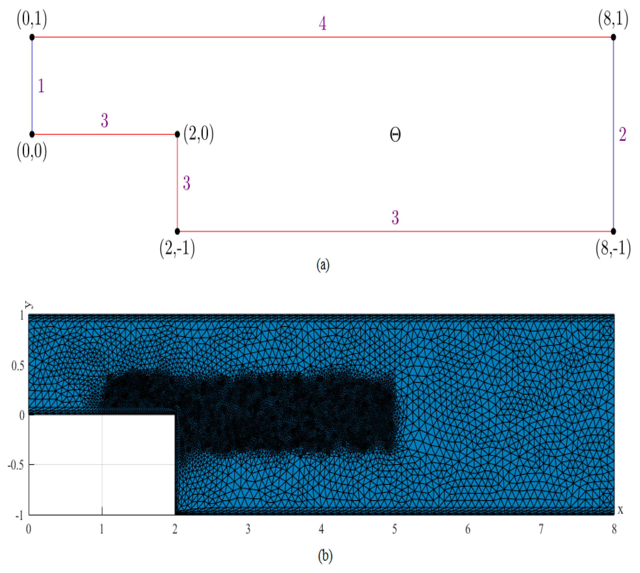
The backwards-facing step flow herein is the same as that in Reference [10]. In order to obtain the best numerical simulating result, mesh is refined near the corner. The flow state in the calculation domain $\Omega$ with boundary $\partial \Omega$ is exhibited in Figure 1a. The boundary line 1 is the inlet with the known initial velocity vector ${(1,0)}^T$, but boundary line 2 is a free outlet. The boundary lines 3 and 4 are two rigidity walls without flow. Both the body force vector ${(g_1,g_2)}^T$ and the initial velocity ${(u^0,v^0)}^T$ are equal to ${(0,0)}^T$. Figure 1b is a graph for the triangular elements with the space mesh scale $h=0.0001$ on the calculation domain $\overline{\Omega }$. The FE subspace ${\mathbb{U}}_h$ consists of the piecewise linear polynomials, the Reynolds number $Re=1000$, and the time step $\Delta t=0.01$.

Figure 1. (a) The calculation region and the boundary values. (b) Spatial mesh on the calculation region.

Noting that ${(g_1,g_2)}^T=\mathbf{0}$ and ${\psi }_h$ and ${\psi }_d$ are linear functions on each element K, so ${\partial }_y{u}_h={\partial }_x{v}_h={\partial }_y{u}_d={\partial }_x{v}_d=0$, by using the first and second equations in Problem 1, the approximate solutions of the pressure p can be calculated with the following formula:

$$\begin{array}{ccc}& & \begin{array}{c}{\displaystyle {\partial }_x{p}_{\delta }^n=-u_{\delta }^n{\partial }_x{u}_{\delta }^n-(u_{\delta }^n-u_{\delta }^{n-1})/\Delta t;}\hfill \\ {\displaystyle {\partial }_y{p}_{\delta }^n=-v_{\delta }^n{\partial }_y{v}_{\delta }^n-(v_{\delta }^n-v_{\delta }^{n-1})/\Delta t,\delta =d\mathrm{or}h.}\hfill \end{array}\hfill \end{array}$$

It follows that

$$\begin{array}{ccc}\hfill & & {\displaystyle p_{\delta ,i,j}^n=0.5[p_{\delta ,i-1,j}^n+p_{\delta ,i,j-1}^n]-0.5h{[u_{\delta }^n{\partial }_x{u}_{\delta }^n+(u_{\delta }^n-u_{\delta }^{n-1})/\Delta t]}_{i,j}}\hfill \\ \hfill & & {\displaystyle -0.5h{[v_{\delta }^n{\partial }_y{v}_{\delta }^n+(v_{\delta }^n-v_{\delta }^{n-1})/\Delta t]}_{i,j},}\hfill \end{array}$$

(37)

where $(\delta =h$ or $d)$ and ${\displaystyle p_{\delta ,i,j}^n=0}$ on $\partial \Omega$. Moreover, ${\displaystyle p_{\delta }(x,y)}$ can also be calculated by the following formula:

$$\begin{array}{ccc}& & {\displaystyle p_{\delta }^n(x,y)=\int ({\partial }_x{p}_{\delta }^n\mathrm{d}x+{\partial }_y{p}_{\delta }^n\mathrm{d}y).}\hfill \end{array}$$

We first obtain the initial 20 CNMFE vorticity coefficient vectors ${\mathbf{\varpi }}_i$ ($i=1,2,\cdots ,$ 20) by solving the CNMFE method at the initial 20 time steps and make up the snapshot matrix $\mathit{A}=({\mathbf{\varpi }}_1,{\mathbf{\varpi }}_2,\cdots ,{\mathbf{\varpi }}_{20})$. Then, according to the way in Section 3.1, we calculate out the eigenvectors ${\mathbf{\varphi }}_j(j=1,2,\cdots ,20)$ corresponding to the eigenvalues ${\lambda }_j$ (arranged degressively) in the matrix ${\mathit{A}}^T\mathit{A}$ that satisfy $\sqrt{{\lambda }_7}⩽{10}^{-4}$. Thereupon, we merely need to take the first six eigenvectors to generate a set of POD bases $\mathsf{\Phi }=({\mathbf{\phi }}_1,{\mathbf{\phi }}_2,\cdots ,{\mathbf{\phi }}_6)$ with ${\mathbf{\phi }}_j=\mathit{A}{\mathbf{\varphi }}_j/\sqrt{{\lambda }_j}$$(j=1,2,\cdots ,6)$. 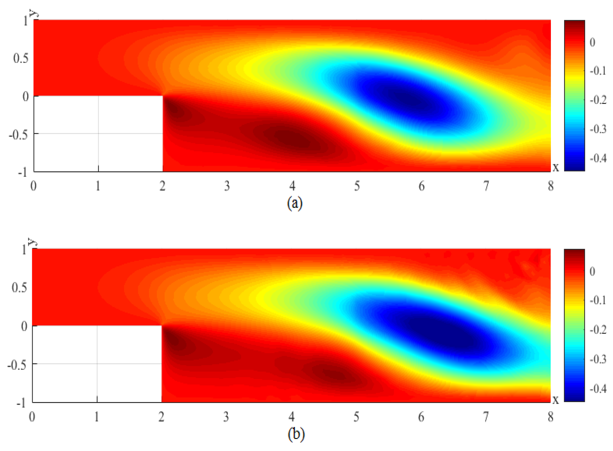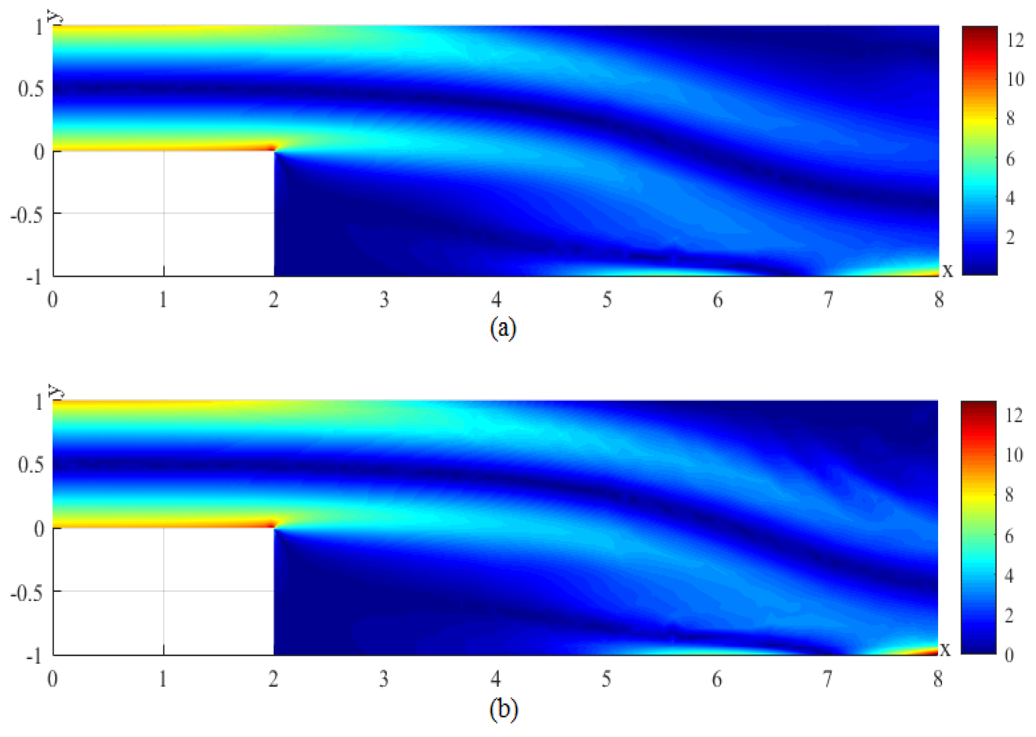Finally, we seek the RDRCNMFE solutions of the components of velocity, the velocity magnitude ($\sqrt{u_d^2+v_d^2}$), and the pressure at $t=4$, 6, 8, and 10 by using Problem 6 and the formula (37), pictured in photo (b) of Figure 2, Figure 3, Figure 4, Figure 5, Figure 6, Figure 7, Figure 8, Figure 9, Figure 10, Figure 11, Figure 12, Figure 13, Figure 14, Figure 15, Figure 16 and Figure 17.

Figure 2. (a) The CNMFE solution for u at $t=4$. (b) The RDRCNMFE solution for u at $t=4$.

Figure 3. (a) The CNMFE solution for v at $t=4$. (b) The RDRCNMFE solution for v at $t=4$.

Figure 4. (a) The velocity magnitude for the CNMFE solution at $t=4$. (b) The velocity magnitude for the RDRCNMFE solution at $t=4$.

Figure 5. (a) The CNMFE solution for p at $t=4$. (b) The RDRCNMFE solution for p at $t=4$.

Figure 6. (a) The CNMFE solution for u at $t=6$. (b) The RDRCNMFE solution for u at $t=6$.

Figure 7. (a) The CNMFE solution for v at $t=6$. (b) The RDRCNMFE solution for v at $t=6$.

Figure 8. (a) The velocity magnitude for the CNMFE solution at $t=6$. (b) The velocity magnitude for the RDRCNMFE solution at $t=6$.

Figure 9. (a) The CNMFE solution for p at $t=6$. (b) The RDRCNMFE solution for p at $t=6$.

Figure 10. (a) The CNMFE solution for u at $t=8$. (b) The RDRCNMFE solution for u at $t=8$.

Figure 11. (a) The CNMFE solution for v at $t=8$. (b) The RDRCNMFE solution for v at $t=8$.

Figure 12. (a) The velocity magnitude for the CNMFE solution at $t=8$. (b) The velocity magnitude for the RDRCNMFE solution at $t=8$.

Figure 13. (a) The CNMFE solution for p at $t=8$. (b) The RDRCNMFE solution for p at $t=8$.

Figure 14. (a) The CNMFE solution for u at $t=10$. (b) The RDRCNMFE solution for u at $t=10$.

Figure 15. (a) The CNMFE solution for v at $t=10$. (b) The RDRCNMFE solution for v at $t=10$.

Figure 16. (a) The velocity magnitude for the CNMFE solution at $t=10$. (b) The velocity magnitude for the RDRCNMFE solution at $t=10$.

Figure 17. (a) The CNMFE solution for p at $t=10$. (b) The RDRCNMFE solution for p at $t=10$.

In order to compare the RDRCNMFE solutions with the CNMFE solutions, by solving Problem 5 and Formula (37), we also compute the CNMFE solutions of the components of the velocity, the velocity magnitude ($\sqrt{u_h^2+v_h^2}$), and the pressure at $t=4$, 6, 8, and 10, pictured in photo (a) of Figure 2, Figure 3, Figure 4, Figure 5, Figure 6, Figure 7, Figure 8, Figure 9, Figure 10, Figure 11, Figure 12, Figure 13, Figure 14, Figure 15, Figure 16 and Figure 17 (where the negative value of v is attributed in the negative y-axis direction). Each pair in Figure 2, Figure 3, Figure 4, Figure 5, Figure 6, Figure 7, Figure 8, Figure 9, Figure 10, Figure 11, Figure 12, Figure 13, Figure 14, Figure 15, Figure 16 and Figure 17 is highly similar, which means that the numerical results of the RDRCNMFE method are sufficiently close to those of the CNMFE method.

In order to further explain the advantage of the RDRCNMFE method, we record the errors of the CNMFE and RDRCNMFE solutions, which are approximately computed by $\parallel u_h^n-u_h^{n+1}{\parallel }_0+\parallel v_h^n-v_h^{n+1}{\parallel }_0+{\parallel p_h^n-p_h^{n+1}\parallel }_0$ and $\parallel u_d^n-u_d^{n+1}{\parallel }_0+\parallel v_d^n-v_d^{n+1}{\parallel }_0+{\parallel p_d^n-p_d^{n+1}\parallel }_0$, respectively, and the CPU running time that solves the RDRCNMFE method and the CNMFE method at $n=400,600,800$, and 1000, listed in Table 1.

Table 1. The errors of the CNMFE and RDRCNMFE solutions and CPU running time.

n	Errors of CNMFE	Errors of RDRCNMFE	CNMFE CPU	RDRCNMFE CPU
	Solutions	Solutions	Running Time	Running Time
400	9.4532$\times {10}^{-4}$	8.1847$\times {10}^{-4}$	56.52143 s	0.83707 s
600	9.6424$\times {10}^{-4}$	8.2953$\times {10}^{-4}$	84.28654 s	1.23136 s
800	9.8648$\times {10}^{-4}$	8.3451$\times {10}^{-4}$	112.04126 s	1.62514 s
1000	1.1321$\times {10}^{-3}$	8.4707$\times {10}^{-4}$	139.84909 s	2.01893 s

The data in Table 1 show that the numerical computing errors for the RDRCNMFE solutions and the CNMFE solutions at four time levels are consistent with the theory errors $O\left({10}^{-4}\right)$, but the RDRCNMFE method can fall off unknowns and shorten the CPU running time because the RDRCNMFE method has only 6 unknowns at each time step, while the CNMFE method has $2\times 14\times {10}^4$ unknowns at the same time step. The data in Table 1 also exhibit that the CPU runtime for finding the RDRCNMFE solutions is far less than that for finding the CNMFE solutions, and it can save time by about a factor of 69. Hence, the RDRCNMFE method is undoubtedly superior over the CNMFE method.

5. Conclusions and Discussions

Herein, we have adopted the POD method to study the reduced dimension of the CNMFE method for the unsteady Navier–Stokes equation. We have built the RDRCNMFE method of the unsteady Navier–Stokes equation by the main few POD bases formed with the first few CNMFE solution coefficient vectors. We have also discussed the stability and errors of the RDRCNMFE solutions by the matrix analysis and used the numerical simulations to verify the advantage of the RDRCNMFE method. The unknowns of the RDRCNMFE method are greatly fewer than those of the CNMFE method, so the RDRCNMFE method can not only highly reduce the computing load and the rounding error accumulation but also highly save the CPU runtime in the computation process. In particular, the reduced dimension for the solution coefficient vectors of the CNMFE method of the unsteady Navier–Stokes equation is proposed for the first time herein. Hence, the RDRCNMFE method is fire-new and distinct from the existing reduced-order methods, such as those mentioned in Section 1. This shows that the RDRCNMFE method for the unsteady Navier–Stokes equation herein is a thoroughly new development.

Although only the RDRCNMFE method for unsteady Navier–Stokes equations is studied in this paper, the method can be applied to other unsteady PDEs, even more complicated actual engineering problems. Hence, the RDRCNMFE method would have very broad applications.