1. Introduction
Queueing theory is a powerful tool for solving the problems of optimal sharing and scheduling limited resources in many real-world systems in the fields of telecommunications, transportation, logistics, emergency services, health-care, computer systems and networks, manufacturing, etc.; for recent references, see, e.g., [
1,
2,
3,
4,
5,
6,
7,
8,
9]. While the main amount of the existing queueing literature is devoted to the systems with homogeneous requests, the efforts of many researches have been focused also on the queueing systems with heterogeneous requests having, in general, different requirements for the service time and different economic value. An important class of such queueing systems assumes the support of a certain system of priorities provided to different types of requests aiming to create more comfortable conditions for requests belonging to the higher-priority classes. Examples of such classes are the urgent (related to safety for life or the security of objects) and non-urgent information in communication networks; handover and new calls in mobile communication networks; primary and cognitive users in cognitive radio systems; injured patients with a danger to their lives or without this in health emergency services; emergency and public or private transport on the roads in the city; preferred or ordinary clients of banks and other systems, etc.
The classical books on priority queues are [
10,
11,
12,
13]. As recent papers dealing with priority queues, the papers [
14,
15,
16,
17,
18,
19,
20,
21,
22] can be mentioned.
In priority queueing systems, usually, requests of different types are stored in different (physically or virtually) buffers. Customers of low priority can be picked up for service only when the buffers designed for higher-priority requests are empty. There is a variety of different priority schemes suitable for modelling and optimising various real-life systems, including non-preemptive (not allowing the interruption of ongoing service), preemptive (allowing the interruption of service), and alternating priorities. Due to the finiteness of the shared resource and the use of work-conserving disciplines, the better are the conditions guaranteed to the high-priority requests, the worse are the conditions provided to the low-priority requests. Traditional, statical, priority schemes suggest that the priority is assigned in advance and does not depend on the queue lengths in the system. Thus, it is possible that, sometimes, there is a very long queue of low-priority requests while the queue of high-priority requests is short. This may not be fair with respect to low-priority requests. Therefore, different strategies of dynamically providing the priorities have been offered in the literature since the paper [
23]; see the survey [
24]. Such strategies suggest that, at any moment of decision-making about the type of the request to be taken for service, this type is defined via some control policy depending on the relation of the queue lengths of different types of requests. A popular class of such policies is monotone policies using thresholds. Other possibilities to make the statical priority more favourable with respect to the low-priority requests are the use of randomisation in the choice (providing, with a certain probability, the chance to a low-priority request to enter the service even in the presence of high-priority requests), the mandatory service of a low-priority request after service, in turn a certain number of high-priority requests, provisioning the weighted service rates, etc.
There are also many works considering the accumulation of priority during a request stay in the queue. For a short review of the corresponding research, see, e.g., the papers [
25,
26]. In [
25], the model with a heterogeneous-batch-correlated arrival process of two types of requests and the phase-type distribution of service time (see, e.g., [
27] for the definition and properties of such a distribution) was analysed. A non-priority request becomes the priority request after its waiting time exceeds some random time having the phase-type distribution. In [
26], the model with the heterogeneous correlated arrival process of an arbitrary finite number of types of requests, a finite common buffer space, the phase-type distribution of the service time, and exponential distributions of times until priority upgrading was analysed. In both of these papers, the arrival flow was assumed to be defined by the Marked Markov Arrival Process (
) (see, e.g., [
28,
29]), which is the generalisation of the well-known Markov Arrival Process (
) to the case of heterogeneous requests. In turn, the
is the significant generalisation of a stationary Poisson arrival process. In contrast to the stationary Poisson arrival process, the
is suitable for modelling, in particular, the flows in the modern communication networks and contact centres that exhibit the correlation and high variability of inter-arrival times. It is already well known that the ignorance of the correlation and high variability of inter-arrival times can lead to huge errors in evaluating the performance and the design of real-world systems. For the literature about the queues with the
, its properties, partial cases, and possible applications see, e.g., [
6,
7,
30,
31,
32,
33,
34,
35,
36,
37,
38]. The literature on the priority queues and
arrival process is still not very extensive. Among the recent papers mentioned above, such an arrival process was assumed in [
14,
18,
20,
22].
In the paper [
39], a new flexible scheme for non-preemptive priority provision was offered. The idea of that scheme is not to define the rule for picking up requests of different priorities from the buffer, but to regulate the rate of admission of these requests to the buffer. This is achieved via managing the auxiliary intermediate buffers for preliminarily storing the arriving requests. The capacities of two intermediate buffers are different, as well as the rates of the transition of requests from these buffers into the main buffer, from which all requests are picked up for service according to First In–First Out (FIFO) principle. Via the proper choice of these rates and capacities, it is possible to provide any degree of priority for requests of both types. Usually considered in the literature, non-preemptive priorities are obtained as a very particular case of this priority scheme.
In this paper, we extended the results of [
39] in two directions. The first direction is the consideration of a multi-server system instead of a single-server system, as analysed in [
39]. Multi-server queueing systems more adequately describe many real-world systems where the shared restricted resource is split into independent units providing service to the requests (operators in call centres, cashiers in stores, logical information transmission channels obtained from a single physical channel via the use of various multiplexing methods, etc.) and are a more difficult subject for investigation. The second direction is avoiding the loss of requests in the case when the intermediate buffers are overloaded. Newly arriving requests to any intermediate buffer seeing that the buffer is full are not lost, as was assumed in [
39], but push the first request from this buffer into the main buffer and occupy the vacant place in the intermediate buffer. This feature allows not only modelling the systems where the loss of requests due to the buffer overflow is not possible, but it allows dynamically giving additional priority to the requests from the currently long queue. As in [
39], we took into account the possible impatience of requests in the intermediate and main buffers because it is well known (see, e.g., [
40]) that requests in many systems exhibit impatience due to various reasons.
The structure of the rest of the paper is as follows. The mathematical model is described in
Section 2. The multidimensional stochastic process describing the behaviour of the considered model is introduced and analysed in
Section 3. In
Section 4, the formulas for the computation of the key performance measures of the system are presented. In
Section 5, the results of the numerical experiment are given.
Section 6 concludes the paper.
2. Mathematical Model
We analysed a queueing system having N independent identical servers and a buffer of infinite capacity. Each server of the system can provide service to two types of requests at rate independent of the type of request.
The arrivals of requests occur according to an
The
is determined by the irreducible continuous-time Markov chain (
)
with the finite state space
The transition rates of this
are defined by the generator, denoted as
The matrix
is represented in the additive form as
where the sub-generator
defines the transition rates of the
, which do not cause requests’ arrival. The non-negative matrix
defines the transition rates of the
which are accompanied with the Type-
k request arrival,
Let
be the invariant probability row vector of the
This vector is computed as the unique solution to the system of linear algebraic equations
Here and further,
denotes a column vector of 1s and
0 denotes a row vector of 0s with the appropriate dimension. The average arrival rate
of Type-
k requests is computed by the formula
The total arrival rate of requests to the system is defined as
Generally speaking, the lengths of the intervals between requests’ arrivals are correlated. The formulas for the computation of the coefficients of variation and correlation can be found, e.g., in [
36]. The methods for the estimation of the parameters of the
describing the flow of requests in some real-world system based on the finite set of the observed request arrival moments (timestamps) were presented, e.g., in [
41].
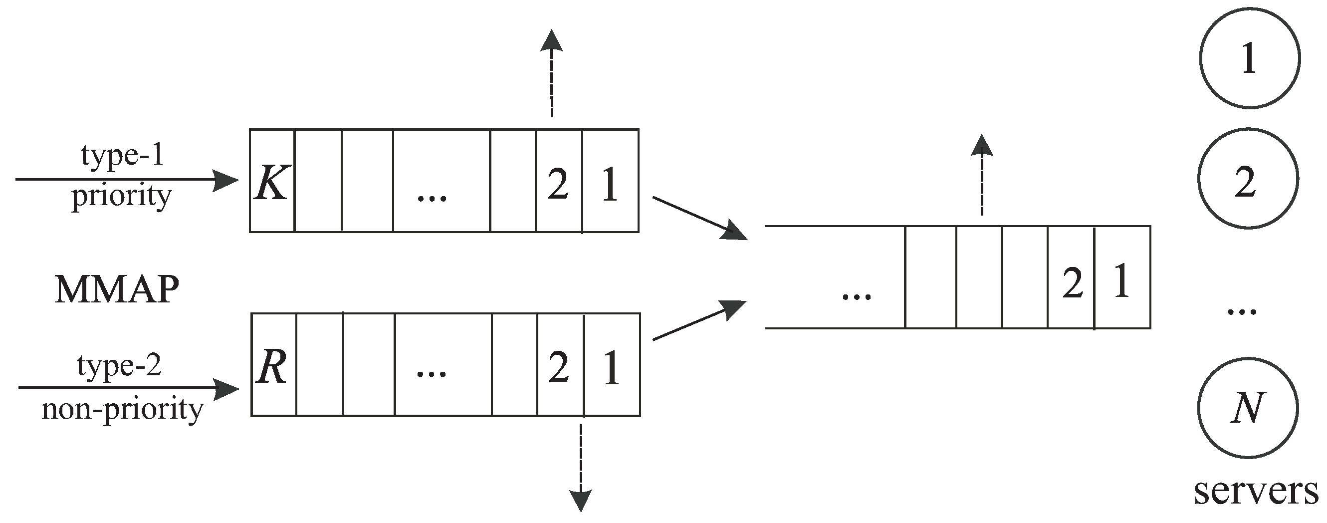
We assumed that Type-1 requests have a priority over Type-2 requests provided via the application of a request admission procedure, described as follows. If the request of any type arrives at the system when at least one server is idle, this request immediately starts service on an arbitrary idle server and, then, after being exponentially distributed with rate time, departs from the system. If an arbitrary Type-k request sees that all servers are busy, it is stored in the kth intermediate buffer, The capacities of the first and second intermediate buffers are equal to K and respectively. If the corresponding buffer is full, this request is placed in the buffer while the first request staying in this buffer is immediately pushed out of the buffer and transits to the main buffer of an infinite capacity. Each request placed in the kth buffer should reside there during exponential time with the rate After this time expires, the request immediately transits to the main buffer. After storing in this buffer, the requests of both types become indistinguishable and are picked up from this buffer for service according to the FIFO principle. If, at some service completion moment, the main buffer is empty, the released server picks up for service the first request from the first buffer, if any. If the first buffer is empty, the offer to start service receives the first request from the second buffer. If all buffers are empty, the server waits until any request arrives at the system, and it will have a chance to start service for this request.
As was proclaimed above, the described admission procedure is flexible in the sense of the degree of the privilege provided to Type-1 requests. The privilege is given via: (i) the order of polling the intermediate buffers when some server becomes idle (the request from the first buffer is invited for service first); (ii) the choice of the rates
of the transition of the requests from the intermediate buffers to the main buffer (rate
can be arbitrarily larger than
); (iii) the proper choice of the capacities of the intermediate buffers. In contrast to [
39], where the small capacity of the buffer might cause the loss of an arriving request and the capacity of the buffer for low-priority requests could be chosen as small, to drop part of these requests, in the model considered in this paper, a small buffer for some type of requests helps to obtain a quicker transition to the main buffer due to the push out mechanism.
Customers staying in the intermediate buffers are impatient. Customers staying in the kth buffer depart from the buffer independently of each other (are lost) instead of transitioning to the main buffer after residing in the buffer while being exponentially distributed with the rate time, Therefore, the large capacity of a buffer and a large impatience rate may stimulate the frequent loss of low-priority requests. Customers staying in the main buffer also can be impatient. The patience time was assumed to have an exponential distribution with the rate After this time expires, the request departs from the system without service (is lost).
The operation of the system is schematically illustrated in
Figure 1.
Our goals were to construct the Markov process describing the behaviour of the system, implement its steady-state analysis, and numerically highlight some dependencies of the system performance measures on the parameters of the model.
3. Random Process Defining the Behaviour of the System
3.1. Selection of the Random Process
Let:
be the total number of requests in service and in the main buffer;
be the number of requests in the first intermediate buffer;
be the number of requests in the second intermediate buffer;
be the state of the underlying process of the
at moment Here, and further, notation like means that the parameter admits values from the set
The four-dimensional
is regular and irreducible. Its infinite state space is defined as
3.2. Generator of the Random Process
To write down the generator of the we need the following denotations:
is the diagonal matrix with the diagonal entries given by the numbers
square matrices and of size l, where or are given by:
;
;
matrices and have all zero entries, except the values and correspondingly, which are equal to 1;
is a row vector of size ;
is the transposed vector ;
⊗ is the symbol of the matrix Kronecker product; see, e.g., [
42,
43,
44];
I is the identity matrix, and O is a square zero matrix of appropriate size. If needed, the size is indicated as the suffix.
To simplify the analysis of the multi-dimensional having one countable component () and three finite components, let us enumerate its states in the direct lexicographic order of the components. We call the set of states of this which have the value i of the countable component as level i of the
Let Q be the generator of the
Theorem 1. The generator Q has the following block-tridiagonal structure:where the non-zero blocks contain the intensities of the transition of the from the states that belong to the level i to the states that belong to the level These blocks are defined as follows: Proof. The proof of Theorem 1 was implemented by means of the analysis of the intensities of all possible transitions of the during the infinitely small time and is presented below.
The block-tridiagonal structure of the generator Q stems from the fact that requests arrive at the system and depart from it (due to service completion or impatience) only one by one.
The form of the non-zero blocks is explained as follows:
The block :
If the system is empty (), that is all three buffers are empty and all servers are idle, the behaviour of the is determined only by the process The intensities of its transitions to other states are equal to the non-diagonal elements of the matrix , and the rates of the exit from the corresponding states are determined up to the sign by the diagonal elements of this matrix. Thus,
The diagonal entries of the blocks :
These entries are negative. Their modules define the exit rate of the from its state. The exit can occur due to the following reasons:
- (a)
The underlying process departs from its current state. The rates of departures are given by the modules of the diagonal elements of the matrix if or matrix if
- (b)
Service completion in one busy server occurs. The rates are given by the diagonal elements of the matrix if or matrix if
- (c)
A Type-1 request departs from the dedicated intermediate buffer due to impatience or transfer to the main buffer. The rates are given by the matrix
- (d)
A Type-2 request departs from the dedicated intermediate buffer due to impatience or transfer to the infinite buffer. The rates are given by the matrix
- (e)
A request departs from the main buffer due to impatience. The rates are given by the matrix
The non-diagonal entries of the blocks :
These entries define the rates of transition of the within the level Such transition rates are given by:
- (a)
Non-diagonal entries of the matrices for or for when the process makes a transition without the generation of a request.
- (b)
Entries of the matrix when a Type-1 request arrives and joins the first intermediate buffer.
- (c)
Entries of the matrix when a Type-2 request arrives and joins the second intermediate buffer.
- (d)
Entries of the matrix when a Type-1 request departs from the intermediate buffer due to impatience.
- (e)
Entries of the matrix when a Type-2 request departs from the intermediate buffer due to impatience.
- (f)
Entries of the matrix when the main buffer is empty at some service completion moment, while the intermediate buffers are not both empty.
The blocks :
These blocks define the rates of transition of the when the number of requests in service or in the main buffer increases from i to
If i.e., there is at least one idle server, this occurs when a request of any type arrives at the system and the request starts service. The transition rates of the process at the moment of a request arrival are determined by the elements of the matrix When the arrived request occupies the last idle server, and from this moment, the numbers of requests in the intermediate buffers should be counted. Row vector fixes that both of these buffers are empty. Therefore, the block is determined by the matrix
Let now The increase of the number of requests in the infinite buffer may occur due to the transition of a request from some intermediate buffer to the infinite buffer. Matrix determines the rate of transition of a request from Buffer 1 to the infinite buffer under the current number of requests in Buffer 1 and the decrease of the number of requests in Buffer 1. No transition of the number of requests in the infinite buffer and underlying process can occur simultaneously with the transition of a request to the infinite buffer. Therefore, the intensities of all transitions of the at the moment of the request transition from Intermediate Buffer 1 to the infinite buffer are given by the matrix By analogy, it may be shown that the intensities of the transitions of the at the moment of the request transition from Intermediate Buffer 2 to the infinite buffer are given by the matrix .
The increase of the number of requests in service and the infinite buffer from i to when can occur also when Buffer 1 is full and a new Type-1 request arrives. This request pushes the first request out of this buffer to the infinite buffer. The rates of transition of the at this moment are determined by the matrix By analogy, it may be shown that the intensities of the transitions of the at the moment of the request being pushed out of Intermediate Buffer 2 to the infinite buffer are given by the matrix As a result, we obtain above-given formula for the block.
The blocks :
The transitions from the level i to the level are possible at the service completion moments (the corresponding rates are given by the matrix , if , or , if ) and the moments of requests’ departure from the infinite buffer due to impatience (the corresponding rates are given by the matrix ). If the service completion leads to emptying one server. Thus, the block admits the form where the column vector is used to cancel the components describing the numbers of requests in Buffer 1 and Buffer 2 (these numbers are equal to zero by default).
Theorem 1 is proven. □
3.3. Ergodicity Condition for the Random Process
Having determined the generator of the , we can proceed to the derivation of the ergodicity condition of this
Theorem 2. The following statements are true.
If the requests residing in the infinite buffer are impatient, i.e., the rate φ is positive, then the is ergodic for an arbitrary set of the parameters of the system.
If the requests in this buffer are patient, i.e., the rate φ is equal to zero, then the criterion of the ergodicity of the is the fulfilment of the inequality:where the vector is the unique solution to the system: Proof. Let us first consider the case
In this case, it is easy to verify that there exist the limits:
where the matrix
is a diagonal matrix with the diagonal entries defined by the corresponding diagonal entries of the matrix
Therefore, the
belongs to the class of continuous-time asymptotically quasi-Toeplitz–Markov chains (
); see [
36,
45]. It follows from [
45] that the sufficient condition for the ergodicity of the Markov chain
is the fulfilment of the inequality:
where the vector
is the unique solution to the system:
It is easy to check that, for the considered with the limiting matrices defined in (4) and (5), it transforms to the evident inequality This proves that the is ergodic for an arbitrary set of the parameters of the system.
Let us now consider the case
In this case, the
is the particular case of the quasi-birth-and-death processes (see [
27]), and the criterion of the ergodicity the
has the form:
where the vector
is the unique stochastic solution to the equation:
Taking into account that and, thus, Inequality (6) reduces to (2).
Theorem 2 is proven. □
Remark 1. It is easy to check that the vector has the following probabilistic sense. When the main buffer is overloaded, the vector defines the joint stationary distribution of the number of requests and the underlying process of in the queueing system with the arrival process, no buffer, two parallel service groups consisting of K and R servers, correspondingly, and the exponential service time distribution in the servers belonging to the rth group with the rate It can be verified that the departure process of successfully serviced requests from this queueing system is the defined by the matrices: The mean departure rate from this system is In the situation when there are many requests in the main buffer, the discussed process of requests’ departure from the system with two service groups defines the arrival process at the main buffer for service in the multi-server system with N servers. Therefore, the process defining the operation of this multi-server system when it is overloaded coincides with the process defining the operation of the system with the defined by the matrices and and the service rate in each server equal to μ. For the former system, it is well known that the ergodicity condition is This inequality, only derived based on intuitive reasoning, coincides with the strictly proven Condition (2) above.
Remark 2. It can be verified that the obtained Condition (2) in the case of a single server (i.e., ) does not coincide with the condition derived for a single-server queue in [39]. This is explained by the different assumptions about the fate of a request arriving when the dedicated intermediate buffer is full. Such a request is assumed to be lost in [39], while in the model under study in this paper, this request pushes out of the intermediate buffer the first request staying there, which joins the main buffer. 3.4. Computation of the Stationary Distribution of the Random Process
Let the condition for the ergodicity of the
be fulfilled. This implies that the following limits (stationary of invariant probabilities) exist:
We sequentially form the row vectors
of these probabilities as:
It is well known that the stationary probability vectors
satisfy the system of equilibrium (or Chapman–Kolmogorov) equations:
In the case of the patient requests in the infinite buffer (
), the way of solving this infinite system is well known; see [
27,
36]. In particular, the vectors
are computed by the formula:
where the matrix
is the minimal non-negative solution of the nonlinear matrix equation:
The vectors are computed as the unique solution to the finite sub-system of equilibrium equations.
In the case of the impatient requests in the main buffer (
), the solution of this infinite system is much more involved. However, it can be solved using the numerically stable methods developed for the
; see [
45,
46,
47].
5. Numerical Examples
The arrival flow of requests was modelled by the
arrival process defined by the following matrices:
The total rate of requests’ (priority and non-priority) arrival at the system is The coefficient of correlation of successive inter-arrival times in this arrival process is and the squared coefficient of variation is . The average intensity of priority (Type-1) requests’ arrival is and the average intensity of non-priority (Type-2) requests’ arrival is .
The intensities of impatience in the first and the second buffers are equal to and the intensities of the transitions from the first and the second buffers to the main buffer are and , respectively. The mean service rate is
We present the results of two experiments. In the first experiment, we fixed the capacities of the intermediate buffers and show the impact of the number of servers N and the impatience rate in the main buffer. In the second experiment, we fixed the values of N and and demonstrate the effect of changing the capacities K and R of the intermediate buffers.
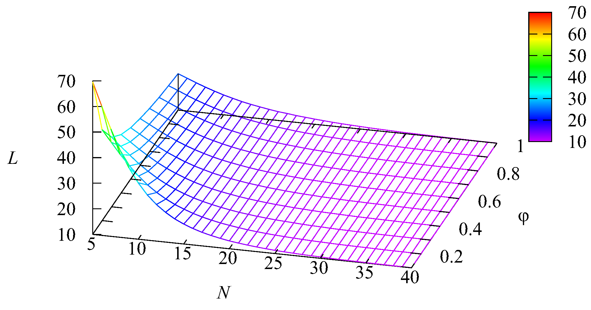
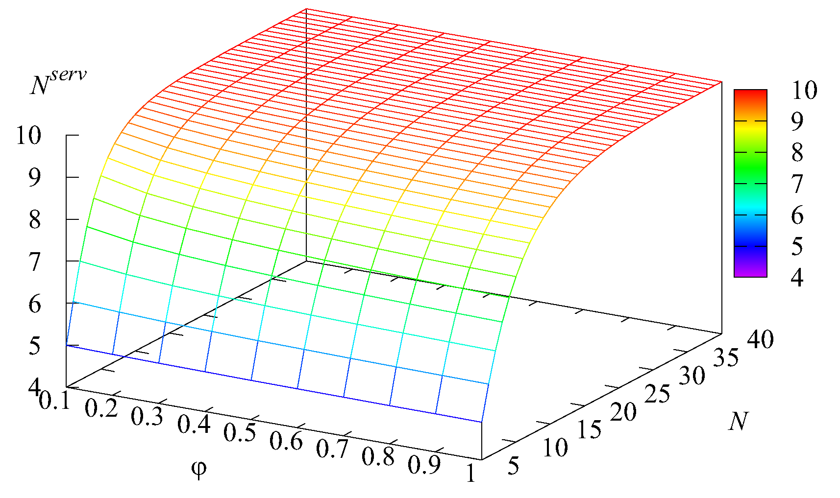
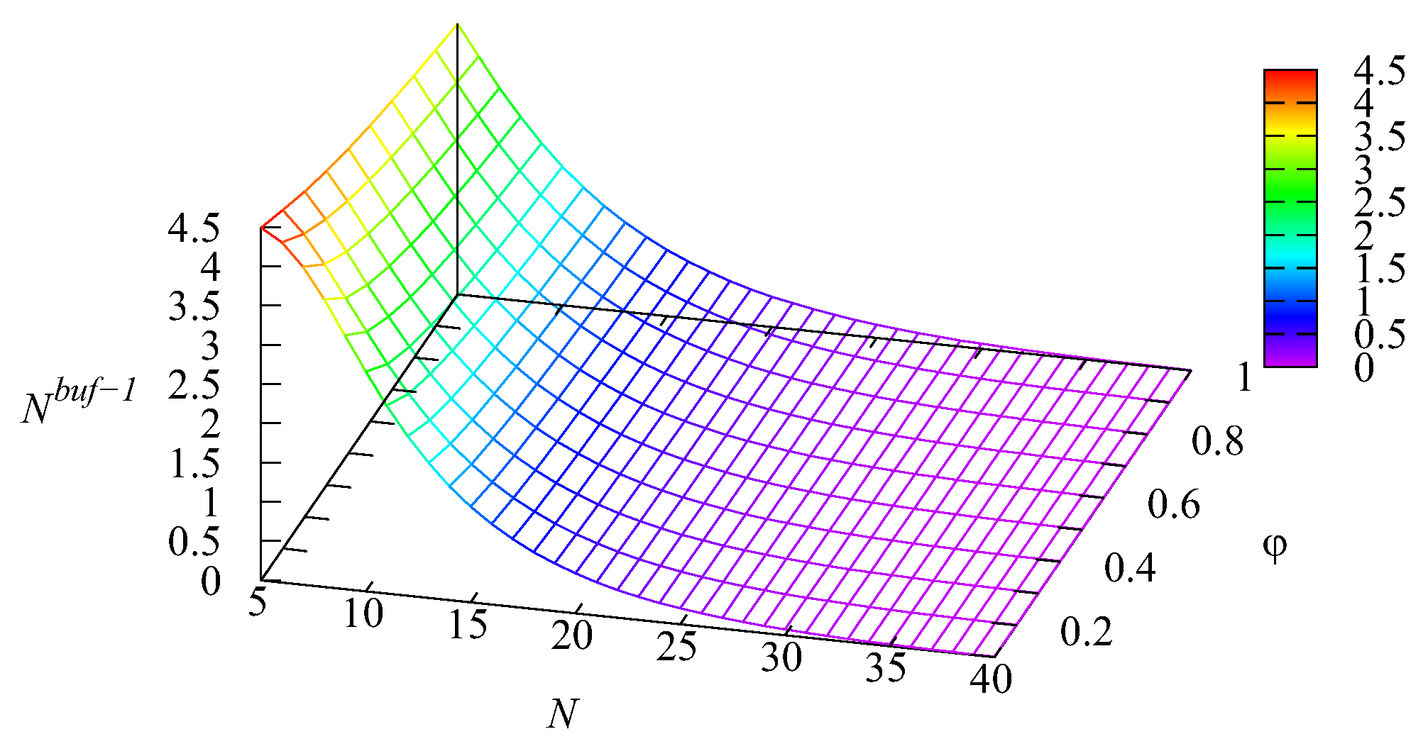
Experiment 1. We assumed that the capacities of the intermediate buffers are for priority requests and for non-priority requests. Let us vary the intensity of the impatience over the interval [0.1,1] with a step of 0.1, and the number of servers N was varied over the interval with a step of 1.
Figure 2,
Figure 3,
Figure 4 and
Figure 5 illustrate the dependence of the mean number of requests in the system
L, the mean number of busy servers
, and the mean number of requests
in the first buffer and
in the second buffer on the values of the intensity
and the number of servers
It is evidently seen in
Figure 2 that the mean number of requests in the system
L is huge (about 70) when the number
N of servers is relatively small (
) and the impatience rate
is also small. An explanation of this fact follows from
Figure 3. It is seen in this figure that, when the number
N of servers is 5, the average number
of busy servers is close to 5. This means that all available servers are practically always busy. It is well known that, in such a situation, the queue length is very long. Because the average number of requests in the main buffer
is the summand in the right-hand side of the expression
it is easy to understand why
L is huge when the number
N of servers and the impatience rate are small. As expected, the value of
L and all summands essentially decrease when the number of servers
N and impatience rate
increase. For large values of
N (
), the mean number of busy servers reduces to about 10, while the values of other summands become practically negligible. The influence of the impatience rate
is essential only when the number
N of servers is small. When it is sufficiently large, service is provided quickly, the main buffer is practically always empty, and requests very rarely depart from this buffer due to impatience.
It should be noted, based on
Figure 4 and
Figure 5, that the average number
of requests residing in the second buffer is essentially larger than the mean number
of requests in the first buffer. This takes place because the arrival rate at the second buffer is 2.33-times higher than the arrival rate at the first buffer and due to the priority provided to Type-1 requests via the higher transition rate to the main buffer and the smaller capacity of the intermediate buffer. For a small number
N of servers, on average, only about 45 percent of the first buffer is occupied. The average percentage of occupation of the second buffer is about 1.9-times higher.
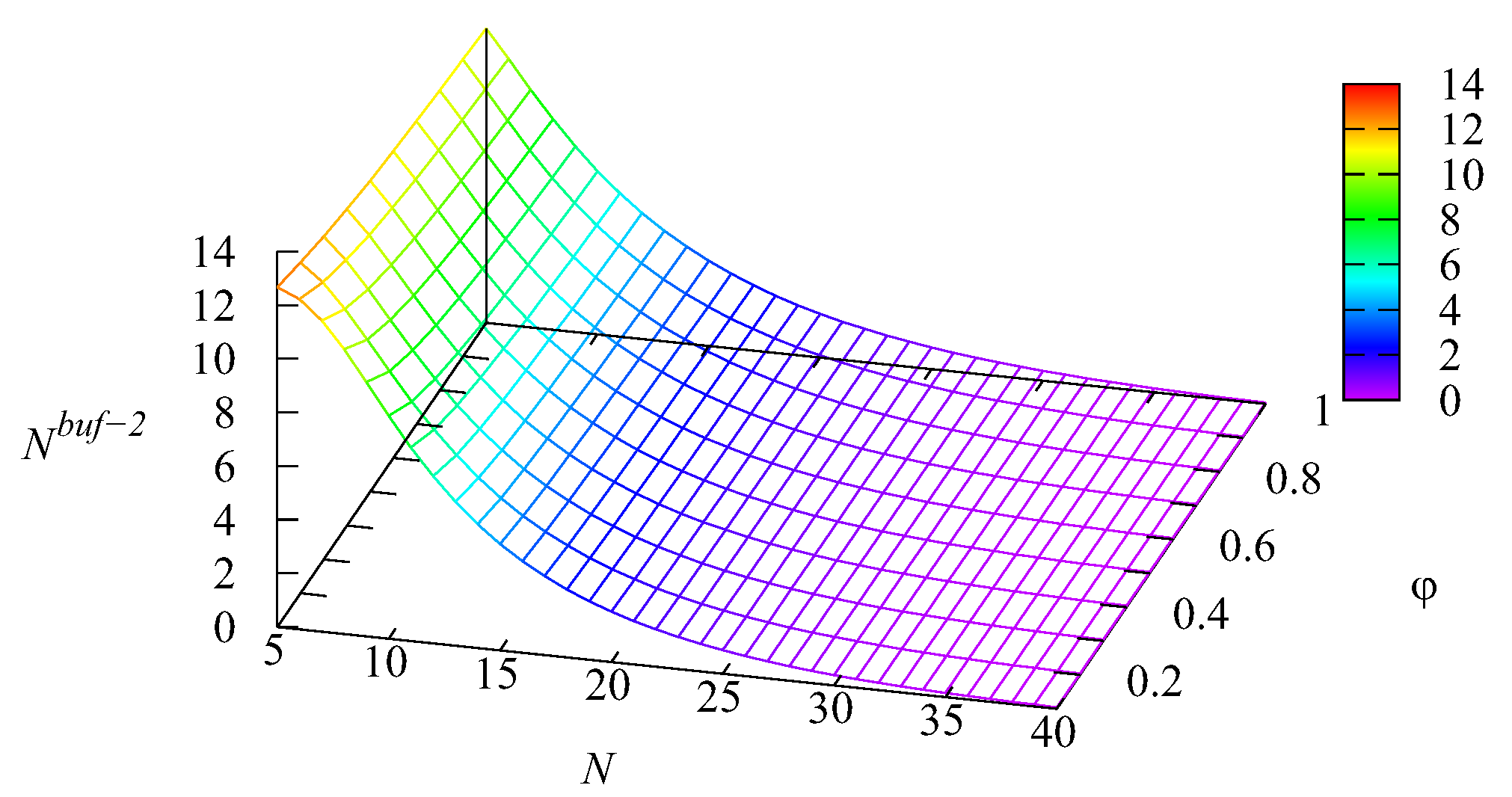
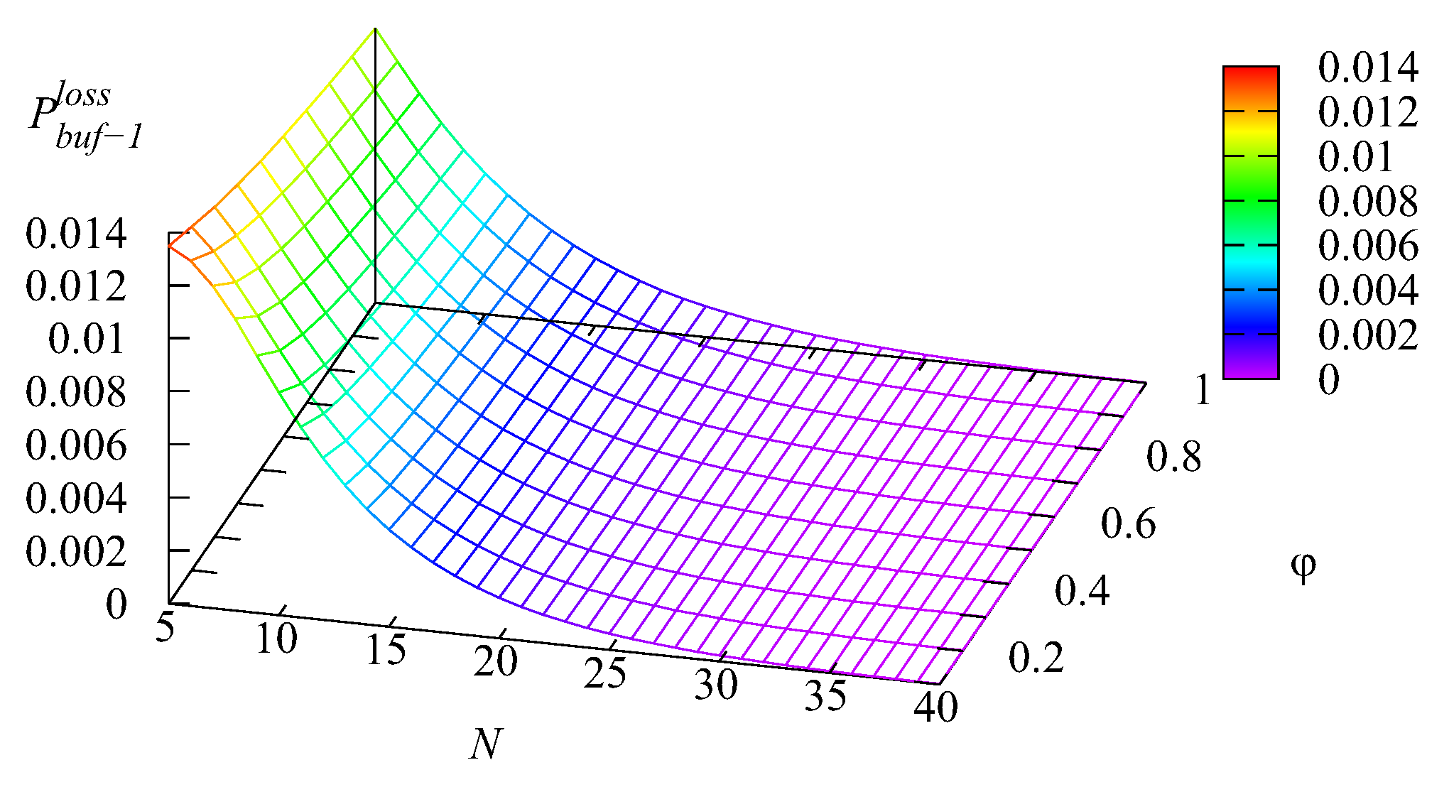
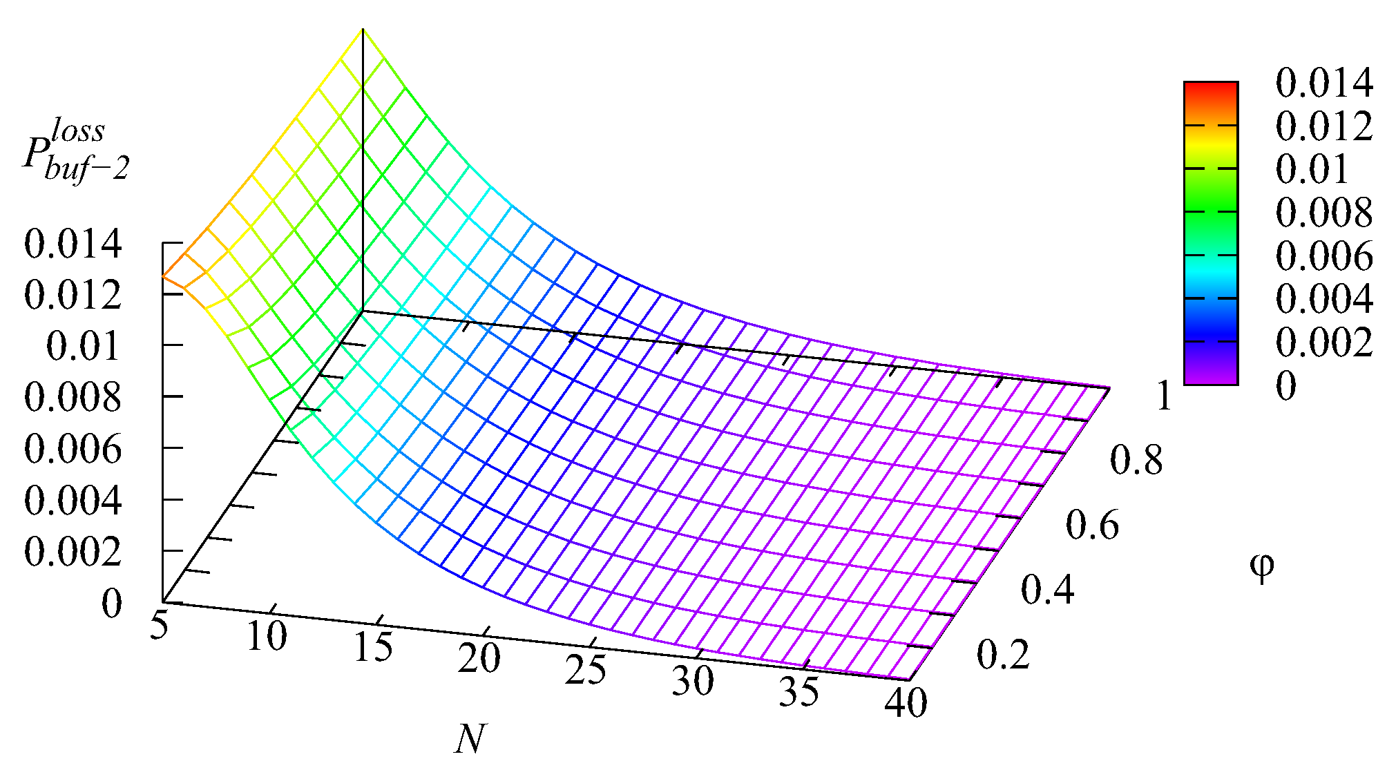
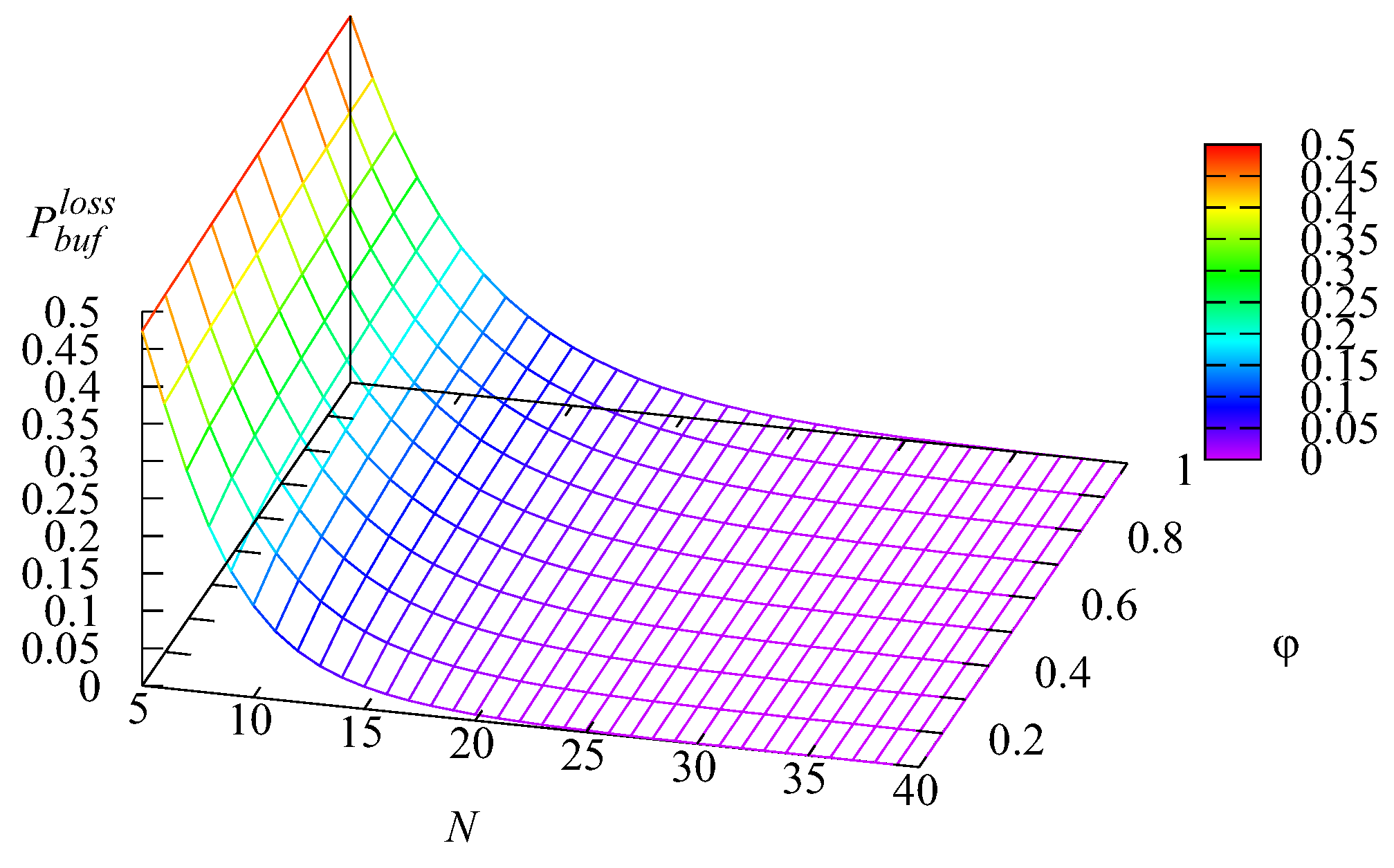
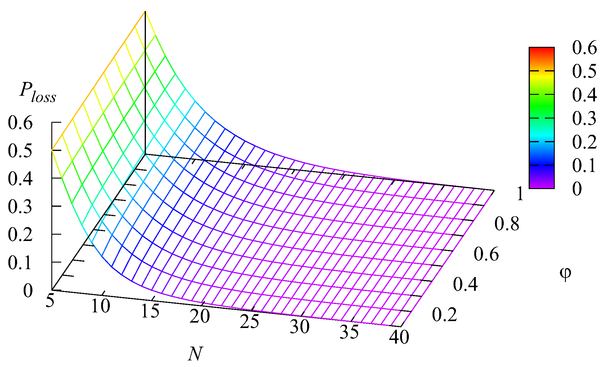
Figure 6,
Figure 7,
Figure 8 and
Figure 9 illustrate the dependence of the loss probability
of an arbitrary request from the first buffer, the loss probability
of an arbitrary request from the second buffer, the loss probability
of an arbitrary request from the main buffer, and the loss probability of an arbitrary request
(all these losses occur due to impatience) on the values of the rate of impatience
and the number of servers
The shapes of the surfaces presented in these figures are similar to the shapes of surfaces presented in
Figure 2,
Figure 3,
Figure 4 and
Figure 5. This was as anticipated because all the mentioned losses occurred due to impatience, and thus, the probabilities
and
of the losses from the two intermediate buffers and the main buffer were proportional (with the weights defined by the respective impatience rates) to the mean number of requests in each buffer. The probability
of an arbitrary request loss is the sum of the loss probabilities
and
, which is confirmed by
Figure 6,
Figure 7,
Figure 8 and
Figure 9. It may be concluded from these figures that all loss probabilities essentially depend on
The dependence on
is weaker, especially for the loss probabilities from the intermediate buffers.
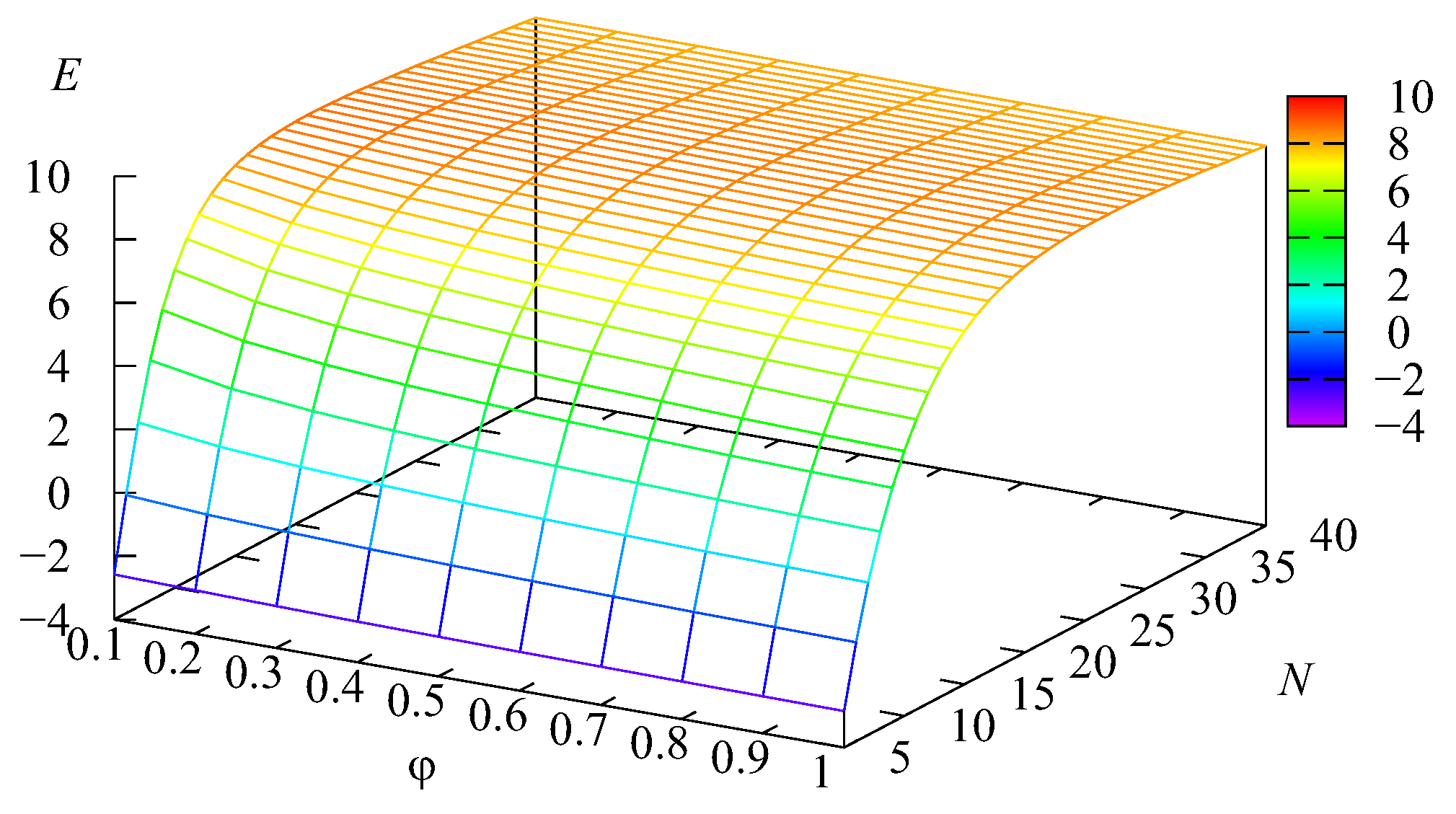
Let us briefly illustrate the possibility of the use of the obtained results for the managerial goals. We considered the problem of the optimal choice of the number
N of servers to maximise the profit of the system. It was assumed that the profit earned by the system during a unit of time under the fixed number
N of servers is evaluated by the profit function:
where
a is the profit gained via service provision to one request,
is the penalty of the system paid for the loss of one request from the
kth intermediate buffer,
c is the penalty of the system paid for the loss of a request from the main buffer, and
d is the cost of the maintenance of one server per unit of time.
Let the cost coefficients
be fixed as follows:
The surface showing the dependence of the cost function
on the number of servers
N and the impatience rate
is presented in
Figure 10.
The optimal values of
N were separately computed for each fixed value of the impatience rate
Table 1 contains the optimal value
of
N and the corresponding optimal value
for ten fixed values of
It is clear that the increase of the impatience rate
implies a larger value of the probability
To decrease this probability, it is necessary to decrease the mean number of requests in the buffer, which can be achieved via the increase of the number of servers
This explains the growth of
when
increases observed in
Table 1. When the number of servers is sufficiently large, the servers succeed in providing service at such a speed that the queue length in the main buffer is very small and the increase of the impatience rate
practically does not have an impact on the value of the profit function.
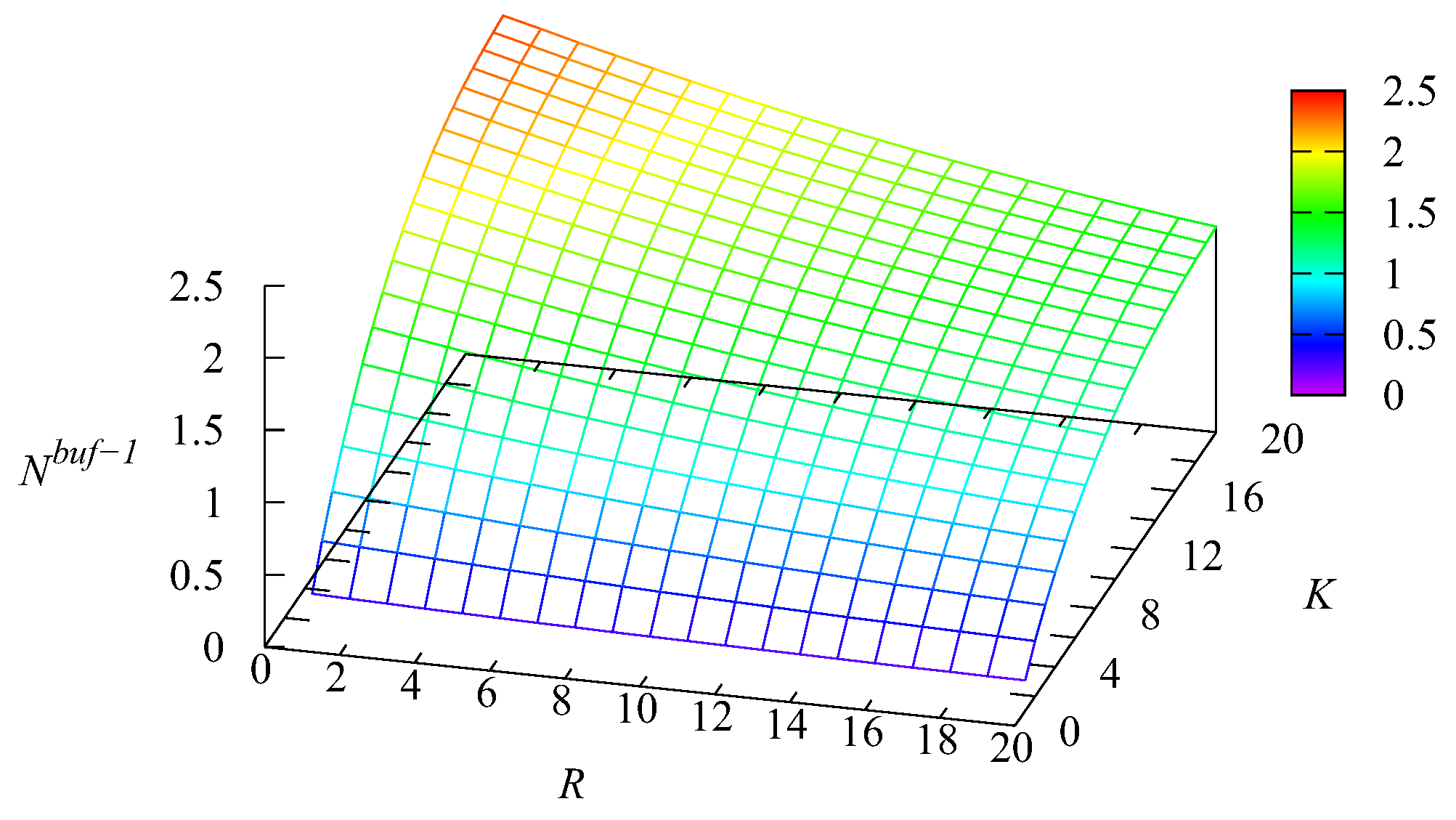
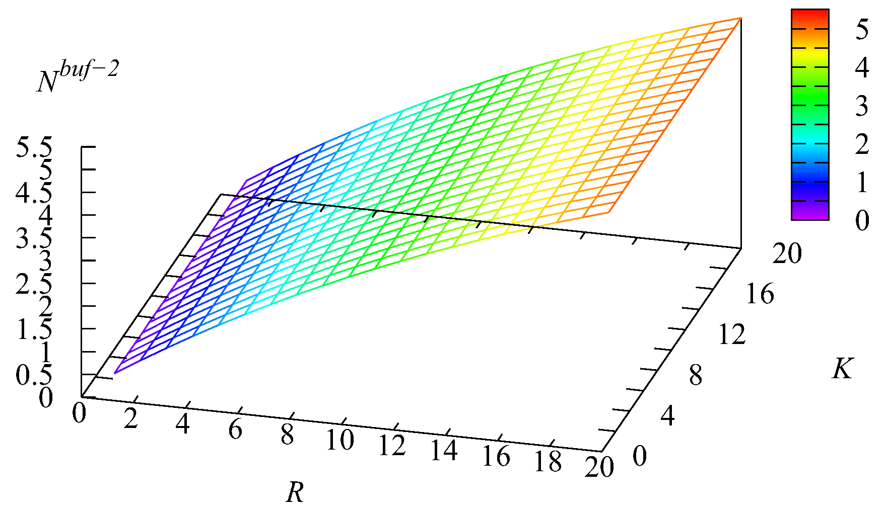
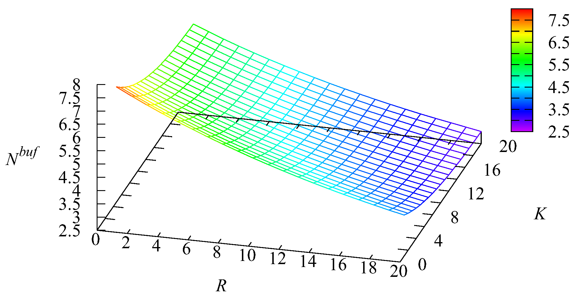
Example 1. Let us now fix the number of servers and the impatience rate in the main buffer To show the impact of the capacities of the intermediate buffers R and we computed the values of various performance measures for the values of R and K varying in the range from 1 to 20 with a step of one.
Figure 11,
Figure 12 and
Figure 13 illustrate the dynamics of the mean number of requests
and
in the first and second buffers and the mean number of requests
in the infinite buffer.
It is natural that the value of the mean number of requests in the first buffer increases when the capacity K of this buffer increases. The essential growth of when the capacity R of the second buffer decreases is explained as follows. When R decreases, more Type-2 requests are pushed out from the second buffer due to the arrival of new Type-2 requests. Therefore, the probability that the main buffer is empty decreases and the chances of Type-1 requests to realise their priority via the privilege to be taken for service when the main buffer becomes empty decrease. This leads to the increase of The maximum of the mean number of requests in the second buffer is essentially larger than the maximum of This occurs due to the higher arrival rate of Type-2 requests and the lower rate of transition from the intermediate buffer to the main one. However, the influence of the relation of the capacities of the intermediate buffers is also high. If R is small, clearly, this reduces the part of the priority of Type-1 requests achieved via their higher rate of transition from the intermediate buffer to the main buffer.
The maximum of the mean number of requests in the main buffer is achieved for a small capacity R of the second buffer. The arrival rate at this buffer is essentially higher than at the first buffer, and a small R leads to the short stay of Type-2 requests in the second buffer before being pushed out to the main buffer. When both K and R are larger, requests stay in the intermediate buffer during a more or less long time. This long delay reduces the burstiness of the flow to the main buffer (we remind that the coefficient of correlation in the arrival process is about 0.3, which is rather large), while it is known in the literature that lower burstiness (or higher regularity) in the arrival process leads to a shorter queue in the system.
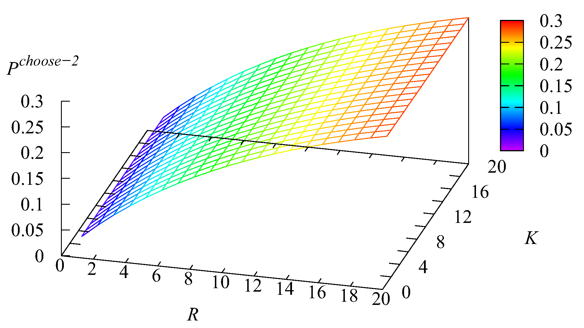
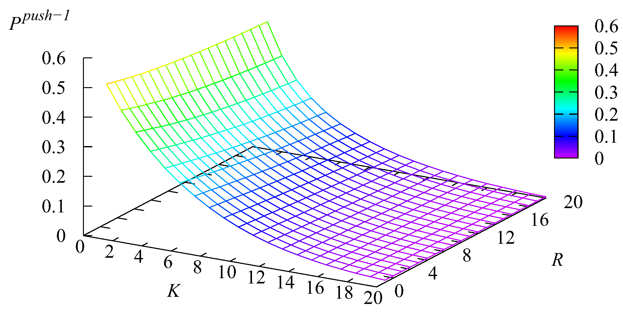
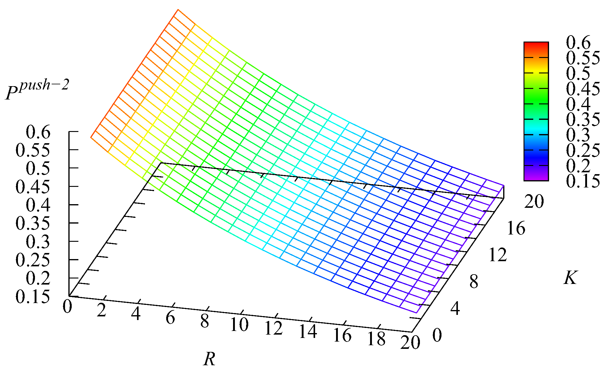
Figure 14 and
Figure 15 depict the dependence of the probability
that an arbitrary Type-
k request will be selected for service from the
k buffer,
without visiting the main buffer on
K and
Recall that, for Type-1 requests, this can happen if all
N servers are busy, the main buffer is empty, the service in one of the servers is completed, and the first intermediate buffer is not empty. For Type-2 requests, this can happen if all
N servers are busy, the main buffer is empty, the service in one of the servers is completed, the first intermediate buffer is empty, and the second intermediate buffer is not empty.
Figure 14 correlates with
Figure 13. When
K and
R are large, the mean number
is the minimal. Thus, the probability that the infinite buffer is empty at the moment of a server releasing is high and the probability
is large. Analogously, when
K and
R are small (the main role is played by the capacity
R of the intermediate buffer, which stores a more intensive flow of Type-2 requests), the mean number
is the max. Thus, the probability that the infinite buffer is empty at the moment of a server releasing is small, and correspondingly, the probability
is small. The growth of
with the increase of
K (which is sharper when
K is still relatively small) stems from the increase of the probability that the first buffer will not be empty at the moment of a server releasing. The reason for the growth of
with the increase of
R is similar. The impact of the variation of
K on the value of
is weak.
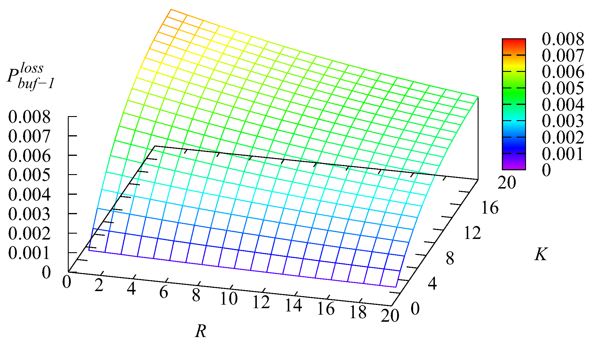
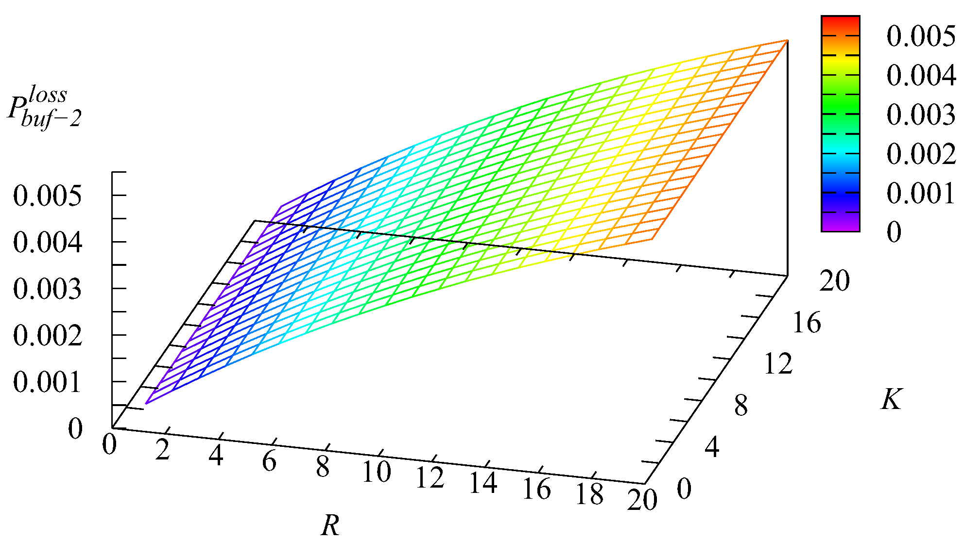
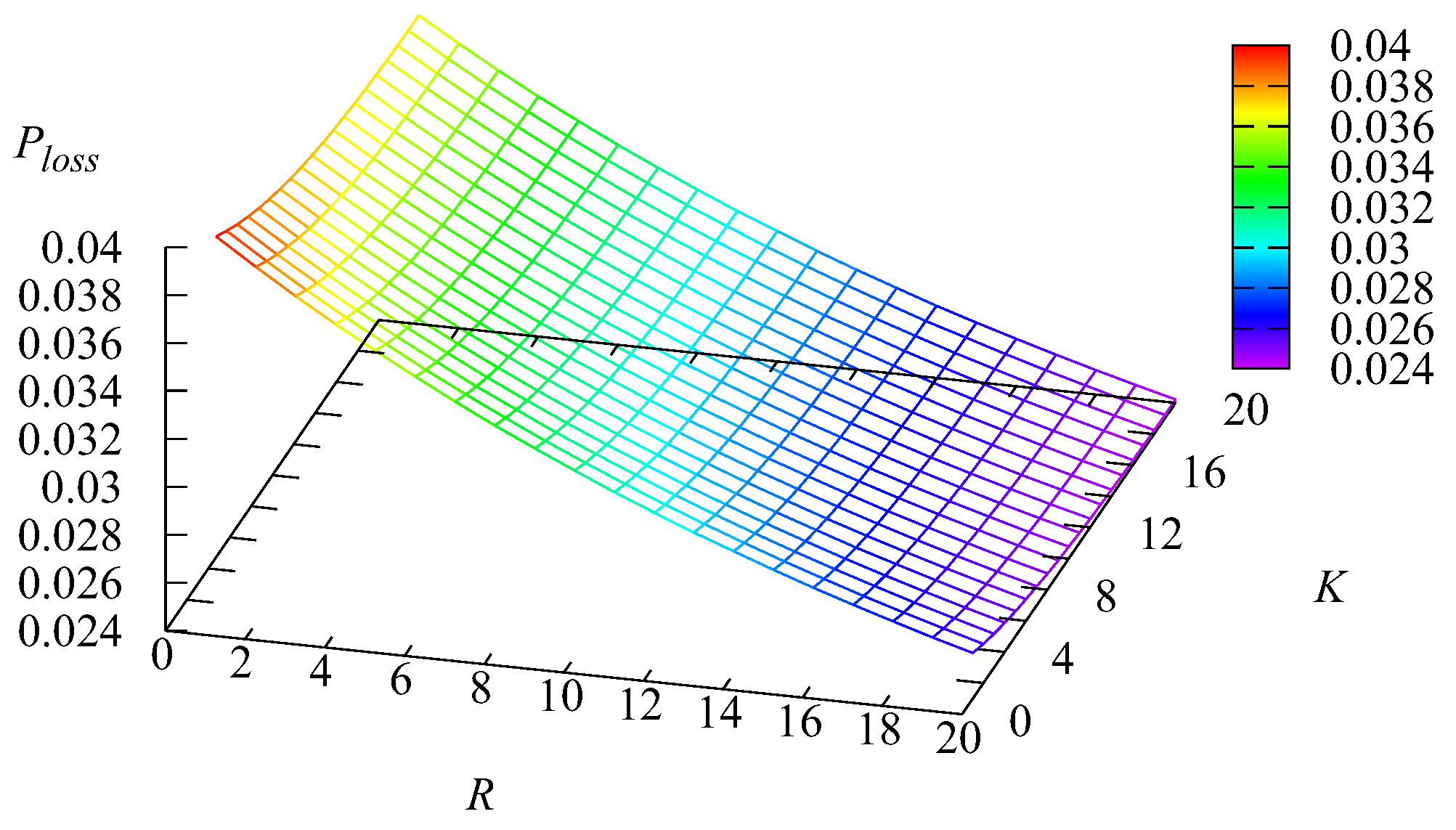
Figure 16,
Figure 17,
Figure 18 and
Figure 19 show the dependence on
K and
R of the following loss probabilities: the probabilities
of an arbitrary request loss from the
kth buffer,
the probability
of an arbitrary request loss from the main buffer, and the probability
of an arbitrary request loss.
Because an arbitrary request loss in the intermediate buffer is due to impatience, it is clear that the loss probability
increases with the increase of the capacity of the
kth intermediate buffer,
Because the capacities of these buffers are relatively small and the impatience rate in the infinite main buffer is larger compared to the rates in the intermediate buffers, the probability
of an arbitrary request from the main buffer also is larger. As is seen from
Figure 16,
Figure 17,
Figure 18 and
Figure 19, this probability is a dominating summand at the right-hand side of the relation
The decrease of the probability
when the capacity
R grows is explained by the the increase of the probability
, leading to the decrease of the arrival rate at the main buffer, the decrease of the queue length in this buffer, and eventually, the decrease of the rate of requests’ departure from the main buffer due to impatience.
The dependence of the probabilities
that an arbitrary Type-
k request upon arrival in the system will find the
kth buffer full,
and the first request from this buffer will go to the main buffer on
K and
R is shown in
Figure 20 and
Figure 21.
As expected, the probabilities are maximal when the capacity of the kth buffer is small and essentially decrease when this capacity increases. Furthermore, these probabilities are weakly sensitive with respect to the capacity of another buffer.


