Abstract
In this paper, open queuing networks with Poisson arrivals and single-server infinite buffer queues are considered. Unlike traditional queuing models, customers are served (with exponential service time) in batches, so that the nodes are non-work-conserving. The main contribution of this work is the design of an efficient algorithm to find the batch sizes which minimize the average response time of the network. As preliminary steps at the basis of the proposed algorithm, an analytical expression of the average sojourn time in each node is derived, and it is shown that this function, depending on the batch size, has a single minimum. The goodness of the proposed algorithm and analytical formula were verified through a discrete-event simulation for an open network with a non-tree structure.
MSC:
60K20
1. Introduction
The recent growing interest in queuing networks with batch services is motivated by their use as mathematical models of packet switching networks [1], wireless sensor networks [2], manufacturing systems [3,4,5,6], Web servers [7], data-processing systems [8] and transportation systems [9].
The analysis of queues with batch services was originally introduced in [10,11] and extended to queuing networks in [12]. A review of the main results on queues with batch services can be found in [13,14].
Such a feature as batch service significantly complicates the model analysis, since it violates the one step assumption, which is at the basis of product-form queuing networks. Indeed, in general it is not possible to obtain a product-form of the stationary distribution [6,15] for a queuing network with batch services, and this consideration strongly limits their practical applicability. To overcome this problem, approximate analysis methods, based on mean value analysis (MVA) [1] or the decomposition method [6,16], have been proposed in the literature. In [15], an infinitesimal operator was constructed to obtain a stationary distribution. In [17,18,19,20,21,22], a product form of the stationary distribution for queuing networks was obtained under certain assumptions. In more detail, Chao et al. [18] supposed that at service completion, the entire batch coalesces into a single unit, and it either leaves the system or goes to another node according to given routing probabilities; the product-form solution of such a model can provide relevant bounds for the behavior of assembly processes, especially when the system is operating under heavy traffic. In [19], conditions were obtained under which Markovian queues (i.e., with Poisson arrivals of batches of tasks and exponential task-service times), with both batch arrivals and departures, have a geometric queue length probability distribution at equilibrium. Furthermore, in [20], response time density was obtained for a tandem pair of such Markovian queues. Miyazawa and Taylor [21] considered queuing networks with batch arrivals and departures, in which additional batches arrive to the nodes when they are empty. The introduction of these extra arrivals made it possible to obtain a geometric stationary distribution, which is a (stochastic) upper bound for the original network. Such systems were further analyzed by Chao [22], who proved that the stationary distribution satisfies a set of non-standard partial balance equations and that the extra arrivals are the necessary and sufficient conditions for having a product form solution, as well as for the partial balance equation to hold.
In addition to the above-discussed probabilistic analysis, both theoretical [23,24] and practical [3,4,5,8,25] parameter optimization of queuing networks with batch services represent open issues of significant relevance. In more detail, one of the classes of optimization problems involves determining the optimal size of the batch, since it has a significant impact on network performance. Rabta and Reiner [3] proposed a general-purpose genetic algorithm and an approximate decomposition procedure for determining optimal batch sizes in a multi-product manufacturing system with the goal of minimizing the total cycle time. The problem of determining the optimal buffer size in a material handling system with constraints on throughput and cycle time was addressed in [4] by using queue decomposition and an iterative method. In more detail, in a material handling system a vehicle moves back and forth between consecutive workstations that have input/front and output/rear buffers. The system was analyzed as an open queuing network, in which input buffers corresponded to single-server queues with batch arrivals, workstations were modeled as traditional single-server queues and the output buffers corresponded to queues with batch services.
In [5], a queuing network with batch services was used to model semiconductor fabrication facilities. A procedure for distributing plant resources was proposed, which ensures the minimum cost of equipment for a given set of technical characteristics (volume and cycle time targets). Kar and Harrison [8] investigated data processing systems: the optimization problem of finding the batch size by maximizing the throughput was solved using mean-field techniques. Finally, [25] dealt with queues with bulking threshold a and maximum service capacity b; by means of renewal theory, busy period analysis and decomposition techniques. It was shown how increasing the bulking threshold affects performance indexes, such as the mean waiting time and the time-averaged number of loss customers. Then, a necessary and sufficient condition for the optimal bulking threshold that minimizes the expected waiting time was established, and an algorithm which guarantees to find the optimal threshold in polynomial time was proposed.
This paper extends the results published in [15,26] for queuing networks consisting of systems, where b denotes the batch size. In more detail, in [26], based on the fact that the stationary distributions of the considered queue and an queue with (adequately chosen) state-dependent service rates are identical, a product-form for the stationary distribution of a general queuing network with batch services has been obtained. Taking advantage of our previous result, in this work the analytical expression of the average response time of the queuing network is obtained, and it is shown that it has one minimum. This is the basis for the main original contribution of the paper, represented by an algorithm for finding the optimal batch sizes that minimize the mean response time.
It should be noted that similar results were recently derived in [27] for infinite servers queues: Using the factorial moment generating function, the authors obtained a product-form for the stationary distribution of the system; showed that the stationary distributions of the (i.e., ) and queues are identical; and derived some performance indexes. In general, the assumption of infinite servers simplifies the tractability of queuing systems, and to the best of our knowledge a similar analysis has not been extended to the single server case.
The rest of the paper is organized as follows. Section 2 describes the main features of open queuing networks with batch services, and Section 3 introduces the equivalent Jackson network, originally proposed by the authors in [26]. Then, in Section 4, the expressions of the average sojourn time in each node and of the response time of the network are derived. Section 5 presents the main original contribution of this paper, namely, an optimization algorithm for finding the vector of the batch sizes for which the average response time is minimal. Finally, Section 6 numerically illustrates the original contributions of the paper.
2. Statement of the Problem
The paper deals with large-scale networks with batch services and individual routing of the customers. In more detail, a continuous-time open queuing network N consisting of L nodes, , , and an external traffic source is considered. The arrival process is Poissonian with rate , and customer transitions between nodes , , are described by the routing matrix , , where defines the transition probability from node to node .
As in classic open queuing networks, each node , , consists of an infinite capacity single-server queue, and arriving customers are put in the waiting queue if the server is busy. It is assumed that in node the customers are served in batches of size . In more detail, the server stays idle until customers arrive at the node; if more customers are present in the waiting queue when the server is idle, then customers are selected in any order, while the others remain in the queue. The service times are exponentially distributed with parameter , . At the end of the service, the destination node of each customer, independently of the others, is determined accordingly to the routing probability , , .
The following analysis is based on the assumption that the number of possible destinations from each node is significantly larger than the batch size. Therefore, the simultaneous arrival of two or more customers in a node has an infinitesimal probability, and the input flow in each node of N can be approximated as a Poisson stream of customers with intensity depending on and .
The state of the network is described by a vector , where indicates the number of customers at node . Hence, the state space of the queuing network N can be denoted as .
The first step is to determine the stationary distribution , , for the queuing network N, where the stationary distributions in the nodes , , , can be calculated considering each node in isolation, as originally proved in [26] and briefly summarized in the next section.
3. Single Node Analysis and Equivalent Jackson Network
Let us consider the generic node , , in isolation, with input rate given by
where the vector of visitation rates is the solution of the equation with the normalization condition .
It is easy to derive the equilibrium equations for node :
Let us introduce a birth–death process , equivalent in steady-state probabilities to the Markov process associated with the node . The process is defined on the set of states , with birth rates , which do not depend on the state n, , and death rates , . The state space and the parameters of the process correspond to the state space and the input rate of node defined by Equation (1). To determine the rates , , note that the steady-state probabilities of the birth–death process are given by
where
Let ; if the limit exists, then:
or
The existence of the equivalent birth–death process depends upon the existence of a positive solution of the previous equation, which satisfies the stability condition for each node .
As proved in [26], taking into account the stability condition, Equation (5) has a unique root , belonging to the open interval
which in the general case can be determined numerically. From (4) it follows that
and the service rates , ,…, can be easily derived recursively.
Since the equivalent process can be built for any node , it is possible to define a Jackson network with nodes , equivalent in stationary distribution to the original queuing network N with batch services. According to the previous results for the single node, has state-dependent service rates , where n is the number of customers in the node , , , and its arrival rates and routing probabilities are the same as in the original queuing network N.
Moreover, N and its equivalent network are stable if and only if the utilization coefficient in the node , ,
Under such conditions, the stationary distribution for is given by
where
4. Stationary Response Time
The stationary distribution for allows us to calculate the average values of various performance parameters.
To characterized the queuing network as a whole, the most relevant index is the average time spent by a customer in the queuing network, known as response time:
which is given by the weighted sum of the average sojourn times in all the nodes .
An elegant closed-form expression for the average sojourn time is provided by the following Theorem, which is valid for a generic node , . For sake of simplicity, in the proof of the theorem, the subscript i identifying the node is omitted.
Theorem 1.
The average sojourn time in a queuing system with batch services of fixed size b is given by
where λ is the arrival rate and M is the unique solution of (5), satisfying the stability condition.
Proof of Theorem 1.
By substituting (3) into the first equation of (2), we get
and by taking into account the latter equality:
Having defined , the system (2) can be rewritten as follows:
When taking into account Little’s law and the definition of the average number of customers in the system, the average sojourn time is given by
and by substituting the expressions of the state probabilities given by (10), the previous expression becomes
or rearrange the terms according to the powers of x:
The next step of the proof consists in finding the value of . To this end, the system (2) can be rewritten in the form
By summing up all the equations of this system, we obtain
or
By substituting (9) into (11) and applying the formula for the sum of an infinite geometric progression, the probability of an empty system becomes
The last part of the proof consists in manipulating the expression of , which can be significantly simplified thanks to the specific structure of the state probabilities of the system and the properties of M. In more detail:
or, by rearranging the terms:
and after simple algebraic manipulations:
Applying the formulas for the sums of arithmetic and arithmetic-geometric progressions, we obtain
and, after the inverse substitution of :
The sum of the second, third and fourth terms in the latter equation becomes
and, taking into account the well-known formula:
and the average sojourn time can be rewritten as:
Finally, from Equation (5) it is easy to find that
Therefore, since ,
and then:
Thus, we got expression (8). □
Note that for , the root of the Equation (5) is , and hence in accordance with the well-known result for the queue.
5. Average Response Time Optimization
The average response time is a relevant performance index that depends, as highlighted in the previous section, on the routing matrix and the node sojourn times. The latter depend on the network parameters not only explicitly, but also through the values of the roots of (5).
Assuming that the network structure and the incoming traffic rate are fixed parameters, in this section we propose an efficient algorithm to find the optimal batch size vector , for which the average response time of the queuing network N is minimized.
Our optimization algorithm is based on the following two considerations. Firstly, as shown above, the evolution of each node is independent of the rest of the network in a probabilistic sense: the arrival rate to any node of N does not change when the service discipline (namely, the batch size) changes in other nodes, and the input rates depends only on the routing matrix. Therefore, the problem of finding the minimum average response time of N is decomposed into solving L minimization problems for the functions in the nodes , . Secondly, the function has only one minimum for values of satisfying the stability condition .
As in the previous section, for sake of clarity, in the following we omit the subscript i, since the same considerations are valid for all the nodes. To prove that has one minimum, we treat b as a continuous parameter and calculate the second derivative of with respect to b:
From (6) it is easy to see that M converges to as . Moreover, the sequence of the roots is monotone increasing for any . To prove the latter statement, consider the function
i.e., is the largest root of . Hence:
and
since . This means that for the batch size , the largest solution of must satisfy the inequality , since is continuous and . Hence, the function , again considering b as a continuous variable, has an horizontal asymptote as and is monotone increasing; as a consequence of the existence of a finite limit, its increase rate decreases for sufficiently high values of b, and its second derivative must be negative. Moreover, as shown in the Figure 1, Figure 2 and Figure 3 below for various ratios of and , the function is concave (convex upwards) for all values of b satisfying the stability condition. Furthermore, since , and the average sojourn time is a convex function (and has one minimum).
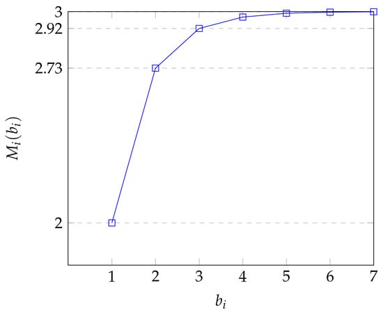
Figure 1.
Limit service rate in the node for , .
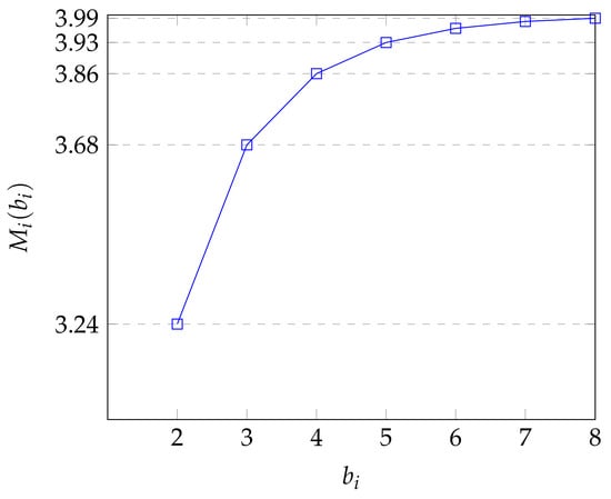
Figure 2.
Limit service rate in the node for , .
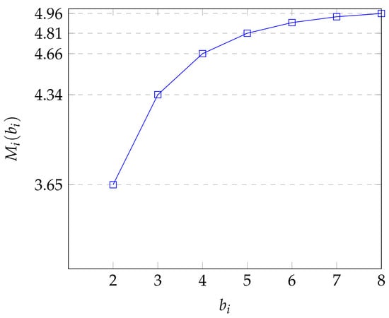
Figure 3.
Limit service rate in the node for , .
Hence, we propose the following optimization algorithm to determine the optimal batch size vector:
- Find the vector solution of equation under the normalization condition .
- Compute the arrival rates vector , as
- Initialize .
- . If , then go to step 14.
- Initialize that represents the iteration number.
- Find the initial value satisfying the condition .
- Find the root of the Equation (5).
- Calculate , where , if and the rates are calculated according to (4), if .
- Calculate the stationary distribution according to (7).
- Calculate the average sojourn time at the node according to (8).
- and increase by 1.
- Repeat steps 7–10.
- If , then go to step 11. If , then decrease by 1 and go to step 4.
- Return the vector b. The algorithm is complete.
6. Numerical Examples
To highlight the correctness of the results in the previous sections, we provide some numerical examples for a single node and a large queuing network, satisfying the assumptions under which the product-form solution was derived.
At first we focus on the sojourn time in a generic node , , with input rate and service rate for batches of customers. Figure 4 and Figure 5 show the behavior of the sojourn time for and , respectively. In more detail, is plotted for different values of (namely, ) as a function of the "allowed" values of the batch size, i.e., the values of satisfying the condition for the existence of a stationary regime.
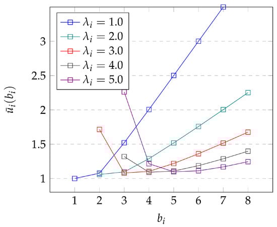
Figure 4.
Average sojourn times in the node for .
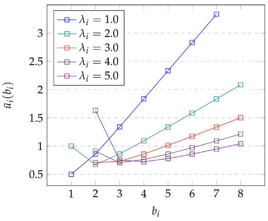
Figure 5.
Average sojourn times in the node for .
Both figures show that the function has one minimum for a specific value of depending on the system’s parameters. For instance, if , then the optimal batch size is one for both values of , whereas for the optimal is already equal to two; and for higher input rates it depends on (compare the graphs for in Figure 4 and Figure 5).
Next, consider the queuing network N, consisting of nodes, with input rate , service rate vector and routing matrix
From the source , the nodes , and may be reached. After being served in these systems, the customers may return to the source (i.e., leave the network) with a probability of 0.5, and with small probabilities equal to 0.1, may move to nodes –. After service is completed in –, the customers may go to with a probability of 0.7 or to one of the nodes – with probabilities equal to 0.1. Finally, customers from – leave the network with sufficiently high probabilities or move to other nodes with the same probability of 0.1.
Links and route probabilities were chosen in such a way that the developed analysis method can be applied. Indeed, small and comparable (in our case, equal) transition probabilities permit one to approximate the input flow, coming to any queue from a large number of nodes, close to a Poisson flow. Moreover, backwards paths (from –) have been introduced to verify the applicability of the proposed methodology also to queuing networks with a non-tree structure.
Using the optimization algorithm proposed in this paper, the optimal batch size vector is . This choice leads to an average response time equal to 7.61, and a mean number of customers in the network equal to 15.22 (in good agreement with the simulation estimates of 7.64 and 15.28, respectively). Here and in the following, all the parameters, derived by discrete-event simulation, were calculated in stationary conditions with a confidence interval of 0.01 and a confidence level higher than 0.95.
For the sake of completeness, Table 1 and Table 2, respectively, show the average number of customers and the average sojourn time in each node of the network. Note that all the analytical values and the corresponding estimates by discrete-event simulation are very close, confirming the applicability of the analytical approach proposed in this paper not only for the whole queue, but also at the node level. In more detail, the largest difference for the average number of customers, observed at node , is less than , whereas for the average sojourn time the maximum was attained at nodes and , and it was equal to .

Table 1.
Average numbers of customers in the nodes.
Table 2.
Average sojourn times in the nodes.
Moreover, Table 2 highlights that the average sojourn times in nodes , and significantly exceed the values in the other nodes of the network. Since in our example the transition probabilities are comparable, this is due to the service rates, which in these nodes are lower than in the rest of the network.
7. Conclusions
In this paper we proposed an efficient method for the analysis of large-scale open queuing networks with batch services and an original algorithm to determine the optimal vector of the service batch sizes, which minimizes the average response time of the network. The proposed algorithm can be used to determine the optimal capacity of vehicles for various purposes, such as the transportation of passengers or goods. The algorithm is also applicable for optimizing systems for the accumulation and subsequent processing of customers requests, which may include information in electronic or paper forms, financial resources, materials, parts and production waste. In more detail, due to the conditions under which the product-form was obtained, the proposed algorithm is applicable to large-scale networks with individual routing of the customers, assuming that the number of possible destinations is significantly larger than the batch size.
Finally, it is worth mentioning that the memory requirement of the algorithm is , and its computational complexity is , where n is the number of the values of the function that must be calculated (in general, n depends on the queuing network parameters).
Author Contributions
Conceptualization, E.S., I.T. and M.P.; methodology, I.T.; software, I.T.; validation, E.S., I.T. and M.P.; formal analysis, E.S., I.T. and M.P.; investigation, E.S., I.T. and M.P.; writing—original draft preparation, E.S., I.T. and M.P.; writing—review and editing, E.S., I.T. and M.P.; visualization, E.S., I.T. and M.P.; supervision, I.T. and M.P.; project administration, E.S.; funding acquisition, E.S. All authors have read and agreed to the published version of the manuscript.
Funding
This work was supported by the Ministry of Science and Education of the Russian Federation in the framework of the basic part of the scientific research state task, project FSRR-2020-0006.
Institutional Review Board Statement
Not applicable.
Informed Consent Statement
Not applicable.
Conflicts of Interest
The authors declare no conflict of interest.
References
- Evequoz, C.; Tropper, C. Approximate analysis of bulk closed queueing networks. Int. J. Prod. Res. 1995, 33, 179–204. [Google Scholar]
- Mitici, M.; Goseling, J.; Ommeren, J.-K.; Graaf, M.; Boucherie, R.J. On a tandem queue with batch service and its applications in wireless sensor networks. Queueing Syst. 2017, 87, 81–93. [Google Scholar] [CrossRef]
- Rabta, B.; Reiner, G. Batch sizes optimisation by means of queueing network decomposition and genetic algorithm. Int. J. Prod. Res. 2012, 50, 2720–2731. [Google Scholar] [CrossRef]
- Yu, A.-L.; Zhang, H.-Y.; Chen, Q.-X.; Mao, N.; Xi, S.-H. Buffer allocation in a flow shop with capacitated batch transports. J. Oper. Res. Soc. 2021, 73, 888–904. [Google Scholar] [CrossRef]
- Hopp, W.J.; Spearman, M.L.; Chayet, S.; Donohue, K.L.; Gel, E.S. Using an optimized queueing network model to support wafer fab design. IIE Trans. 2002, 34, 119–130. [Google Scholar] [CrossRef]
- Hanschke, T.; Zisgen, H. Queueing networks with batch service. Eur. J. Ind. Eng. 2011, 5, 313–326. [Google Scholar] [CrossRef]
- Antunes, N.; Nunes, C.; Pacheco, A. A queueing network with Markov modulated input. In Proceedings of the Second Euro-Japanese Workshop on Stochastic Risk Modelling for Finance, Chamonix, France, 18–20 September 2002; pp. 15–24. [Google Scholar]
- Kar, S.; Rehrmann, R.; Mukhopadhyay, A.; Alt, B.; Ciucu, F.; Koeppl, H.; Binnig, C.; Rizk, A. On the throughput optimization in large-scale batch-processing systems. Perform. Eval. 2020, 144, 102142. [Google Scholar] [CrossRef]
- Grippa, P.; Schilcher, U.; Bettstetter, C. On access control in cabin-based transport systems. IEEE Trans. Intell. Transp. Syst. 2019, 20, 2149–2156. [Google Scholar] [CrossRef]
- Beiley, N.T.J. On Queueing Processes with Bulk Service. J. R. Stat. Soc. 1954, 16, 80–87. [Google Scholar] [CrossRef]
- Downton, F. Waiting time in bulk service queues. J. R. Stat. Soc. 1955, 17, 256–261. [Google Scholar] [CrossRef]
- Henderson, W.; Pearce, C.E.M.; Taylor, P.G.; Dijk, N.M. Closed Queueing Networks with Batch Services. Queueing Syst. 1990, 6, 59–70. [Google Scholar] [CrossRef]
- Sasikala, S.; Indhira, K. Bulk Service Queueing Models—A Survey. Int. J. Pure Appl. Math. 2016, 106, 43–56. [Google Scholar]
- Chaudhry, M.L.; Templeton, J.G.C. A First Course in Bulk Queues; John Wiley & Sons Inc.: New York, NY, USA, 1983. [Google Scholar]
- Stankevich, E.P.; Tananko, I.E.; Dolgov, V.I. Analysis of closed queueing networks with batch service. Izv. Saratov Univ. (N. S.) Ser. Math. Mech. Inform. 2020, 20, 527–533. [Google Scholar] [CrossRef]
- Klunder, W. Decomposition of Open Queueing Networks with Batch Service. In Operations Research Proceedings 2016; Springer: Cham, Switzerland, 2018; pp. 575–581. [Google Scholar]
- Daduna, H. Queueing Networks with Discrete Time Scale: Explicit Expressions for the Steady State Behavior of Discrete Time Stochastic Networks; Springer: New York, NY, USA, 2001. [Google Scholar]
- Chao, X.; Pinedo, M.; Shaw, D. Networks of Queues with Batch Services and Customer Coalescence. J. Appl. Probab. 1996, 33, 858–869. [Google Scholar] [CrossRef]
- Harrison, P.G. Product-form queueing networks with batches. In Computer Performance Engineering, Proceedings of the 15th European Workshop, EPEW 2018, Paris, France, 29–30 October 2018; Lecture Notes in Computer Science; Springer: Cham, Switzerland, 2018; pp. 250–264. [Google Scholar]
- Harrison, P.G.; Bor, J. Response time distribution in a tandem pair of queues with batch processing. J. ACM 2021, 68, 1–41. [Google Scholar] [CrossRef]
- Miyazawa, M.; Taylor, P.G. A Geometric Product-Form Distribution for a Queueing Network with Non-Standard Batch Arrivals And Batch Transfers. Adv. Appl. Prob. 1997, 29, 523–544. [Google Scholar] [CrossRef]
- Chao, X. Partial Balances in Batch Arrival Batch Service and Assemble-Transfer Queueing Networks. Adv. Appl. Prob. 1997, 34, 745–752. [Google Scholar] [CrossRef]
- Neely, M.J. Stochastic Network Optimization with Application to Communication and Queueing Systems; Morgan & Claypool: San Rafael, CA, USA, 2010. [Google Scholar]
- Xia, C.H.; Michailidis, G.; Bambos, N.; Glynn, P.W. Optimal control of parallel queues with batch service. Probab. Eng. Inform. Soc. 2002, 16, 289–307. [Google Scholar] [CrossRef][Green Version]
- Zeng, Y.; Xia, C.H. Optimal bulking threshold of batch service queues. J. Appl. Prob. 2017, 54, 409–423. [Google Scholar] [CrossRef]
- Stankevich, E.; Tananko, I.; Pagano, M. Analysis of Open Queueing Networks with Batch Services. In Information Technologies and Mathematical Modelling. Queueing Theory and Applications, Proceedings of the 20th International Conference, ITMM 2021, Named after A.F. Terpugov, Tomsk, Russia, 1–5 December 2021; Communications in Computer and Information Science; Springer: Cham, Switzerland, 2022; pp. 40–51. [Google Scholar]
- Nakamura, A.; Phung-Duc, T. Stationary Analysis of Infinite Server Queue with Batch Service. In Performance Engineering and Stochastic Modeling, Proceedings of the 17th European Workshop, EPEW 2021, and 26th International Conference, ASMTA 2021, Virtual Event, 9–10 December and 13–14 December 2021; Lecture Notes in Computer Science; Springer: Cham, Switzerland, 2021; pp. 411–424. [Google Scholar]
Publisher’s Note: MDPI stays neutral with regard to jurisdictional claims in published maps and institutional affiliations. |
© 2022 by the authors. Licensee MDPI, Basel, Switzerland. This article is an open access article distributed under the terms and conditions of the Creative Commons Attribution (CC BY) license (https://creativecommons.org/licenses/by/4.0/).