Article

Fractional-Order SEIRD Model for Global COVID-19 Outbreak

1
Department of Mathematics, Faculty of Sciences of Sfax, University of Sfax, Road of Soukra Km 3.5, B.P. 1171, Sfax 3000, Tunisia
2
Department of Mathematics, College of Science for Women, Baghdad University, Baghdad 10071, Iraq
*
Author to whom correspondence should be addressed.
These authors contributed equally to this work.
Mathematics 2023, 11(4), 1036; https://doi.org/10.3390/math11041036
Submission received: 29 December 2022 / Revised: 25 January 2023 / Accepted: 6 February 2023 / Published: 18 February 2023
(This article belongs to the Special Issue Applications of Symbolic and Soft Computations in Applied Sciences)

Abstract

:
With the identification of new mutations in the coronavirus with greater transmissibility and pathogenicity, the number of infected people with COVID-19 worldwide has increased as from 22 June 2021, and a new wave has been created. Since the spread of the coronavirus, many studies have been conducted on different groups. The current research was adopted on the implementations of fractional-order (SEIRD: Susceptible, Exposed, Infected, Recovered, Died) people model with a Caputo derivative for investigating the spread of COVID-19. The characteristics of the system, such as the boundedness, existence, uniqueness and non-negativity of the solutions, the equilibrium points of system, and the basic reproduction number, were analyzed. In the numerical part, a simulation for the spread of the virus is presented, which shows that this wave of spread will continue for the next few months and an increasing number of people becoming infected. Furthermore, the numerical results obtained from several types of fractional-order derivatives are compared with real data, which subsequently shows that the Caputo fractional-order derivative follows real data better than others. In addition, the obtained reproduction number has a value greater than one, indicating a continuation of the disease outbreak and the necessity of taking more control decisions.
MSC:
26A33; 34K37; 35R11

1. Introduction

In late 2019, COVID-19 was first identified in Wuhan, China, and then transmitted through infected people to other countries and spread all over the world. In response, the World Health Organization announced a pandemic within months. The cause of this disease is a type of virus from the family of coronaviruses, which was originally called 2019-nCoV and now, almost 18 months after the identification of this virus, it is termed SARS-CoV-2. Some of the diseases caused by coronaviruses include the common cold and severe illnesses such as Middle East Respiratory Syndrome (MERS) and Severe Acute Respiratory Syndrome (SARS). COVID-19 shows different symptoms in different people. Common symptoms of the disease include fever, cough and respiratory problems, but symptoms such as sore throat, digestive problems, skin symptoms, loss of taste and smell, etc., have also been reported. The primary virus infected most adults, but in late 2020, it was announced that the new species, SARS-CoV-2, would also infect children and adolescents.
The use of mathematical models is a valuable method in the study of natural phenomena, biological systems, computer systems and even economic phenomena (see, for example, Refs. [1,2,3,4,5,6,7]).
Therefore, investigating the spread of COVID-19 and predicting its transmission became one of the most interesting topics for researchers. In these studies, the use of mathematical models as a tool proved useful for many researchers and various subsequent mathematical models were written. According to the objectives of the research and how to transfer COVID-19, various mathematical models have been written such as: the modified SI model (Kosmidis et al. [8]), the SIR model (Cooper et al. [9]), the SIRD model (Martinez [10]), the classical SEIR model (Yousef et al. [11]), the modified SEIR model (Lopez et al. [12]), the network-based stochastic SEIR model (Groendyke et al. [13], the multi-stage SEIR model (Khedher et al. [14]), etc. In these modelings, the ordinary-order derivative was used; however, due to the expansion of the fractional-order derivative in recent decades and the good results of fractional-order derivative modeling, many mathematicians have used the fractional-order derivative in their works, we can refer to the approaches of Almeida et al. [15], Koca [16], Khan et al. [17], Singh [18], Ullah et al. [19], Wang et al. [20], Pakhira et al. [21], Sun et al. [22], Edelstein-Keshet [23], Baleanu et al. [24], Dokuyucu et al. [25], Kumar et al. [26], Ozturk et al. [27], Alkahtani et al. [28], and Pan et al. [29]. Derivatives of fractional-order preserve the internal and historical memory for modeling natural phenomena and have better compatibility with the process of spreading diseases.
In the COVID-19 transmission system, we see that the number of actively infected people always affects the subsequent number of infected people and does not depend only on the initial value. This shows that the COVID-19 transmission system has historical memory, and therefore according to the above discussion, the best choice for modeling the transmission of this disease is the fractional-order derivative. Since the beginning of the COVID-19 outbreak, some researchers have studied COVID-19 transmission using mathematical models with fractional-order derivatives. We can refer to the approaches of Rezapour et al. [30], Alshomrani et al. [31], Khan et al. [32], Lu et al. [33], Baleanu et al. [34], Aba Oud et al. [35], and seda igret Araz [36].
Based on a search within the Scopus database, the implementation of a fractional-order model for COVID-19 analysis has shown 136 research articles. This is evidenced by the capacity of the fractional-order model for solving such a complex societal disease spread. Although, there has been a huge number of studies within the short period of 1.5 years, mathematical scientists remain eager to adopt this model for better understanding of this complex issue. The search of the Scopus database was visualized using VOSviewer algorithm and indicating keywords indices. Figure 1a shows that the fractional-order model has been integrated with several methodologies such as Caputo derivatives, approximate solution, mathematical operators, etc., in order to improve the modeling performance and conduct better analyses. In addition, Figure 1b presented the VOSviewer algorithm indicated that 44 countries conducted this specific type of research. Saudi Arabia and Pakistan were on the top of this list. The literature review analysis revealed the significance of this topic and the capacity of ongoing research in this domain, in which a better mathematical system is to be established for better comprehending the COVID-19 spread or developing reliable emerging technology for stopping the virus spread.
Researchers have employed different models such as SIR, SEIR, SIRD, and SEIRD to investigate the spread of COVID-19. In this article, we use the SEIRD model to study five groups (Susceptible, Exposed, Infected, Recovered, Died) involved with the disease. In the classical model, the total number of people is considered constant and does not have the necessary accuracy in predicting the future disease status. Therefore, to improve the results, we added the natural birth rate and the natural death rate to the model. The spread of COVID-19 has a historical memory and therefore the use of the ordinary derivative that does not preserve the system memory is not suitable for the spread of this disease. Caputo fractional derivative is more compatible with natural phenomena. We used the Caputo fractional-order derivative and compared the results of the model with the three types of fractional-order derivatives. Because the basic reproduction number is of special importance in the study of pandemic diseases; therefore, in the numerical simulation section, we examine the effect of model parameters on it and identify the factors that have the greatest impact on the continuation of disease spread. Furthermore, using simulation with MATLAB software, we provide a forecast for the spread of the disease over the next few months. By plotting the results of the model for several different fractional orders, we examine the effect of the derivative order on the behaviour of the resulting functions.
The rest of the paper is structured as follows: The SEIRD model is presented in Section 2 to investigate the COVID-19 outbreak and the basic features of the system are analyzed. In Section 3, it is proved that the model has a unique solution. Finally, a numerical analysis of the system and a study of the COVID-19 outbreak globally, and the conclusions are presented in Section 4 and Section 5, respectively.

2. The Desired Fractional-Order Model

In this section, we present a box model to analyze the transmission of COVID-19. According to reported information about COVID-19 transmission, people with the disease are divided into two categories: symptomatic and asymptomatic. We divide the whole set of people N ( t ) into five groups: Susceptible people S ( t ) , Exposed or asymptomatic infected people E ( t ) , Symptomatic infected people I ( t ) , Recovered people R ( t ) and people who have died of COVID-19 disease D ( t ) , N ( t ) = S ( t ) + E ( t ) + I ( t ) + R ( t ) + D ( t ) .
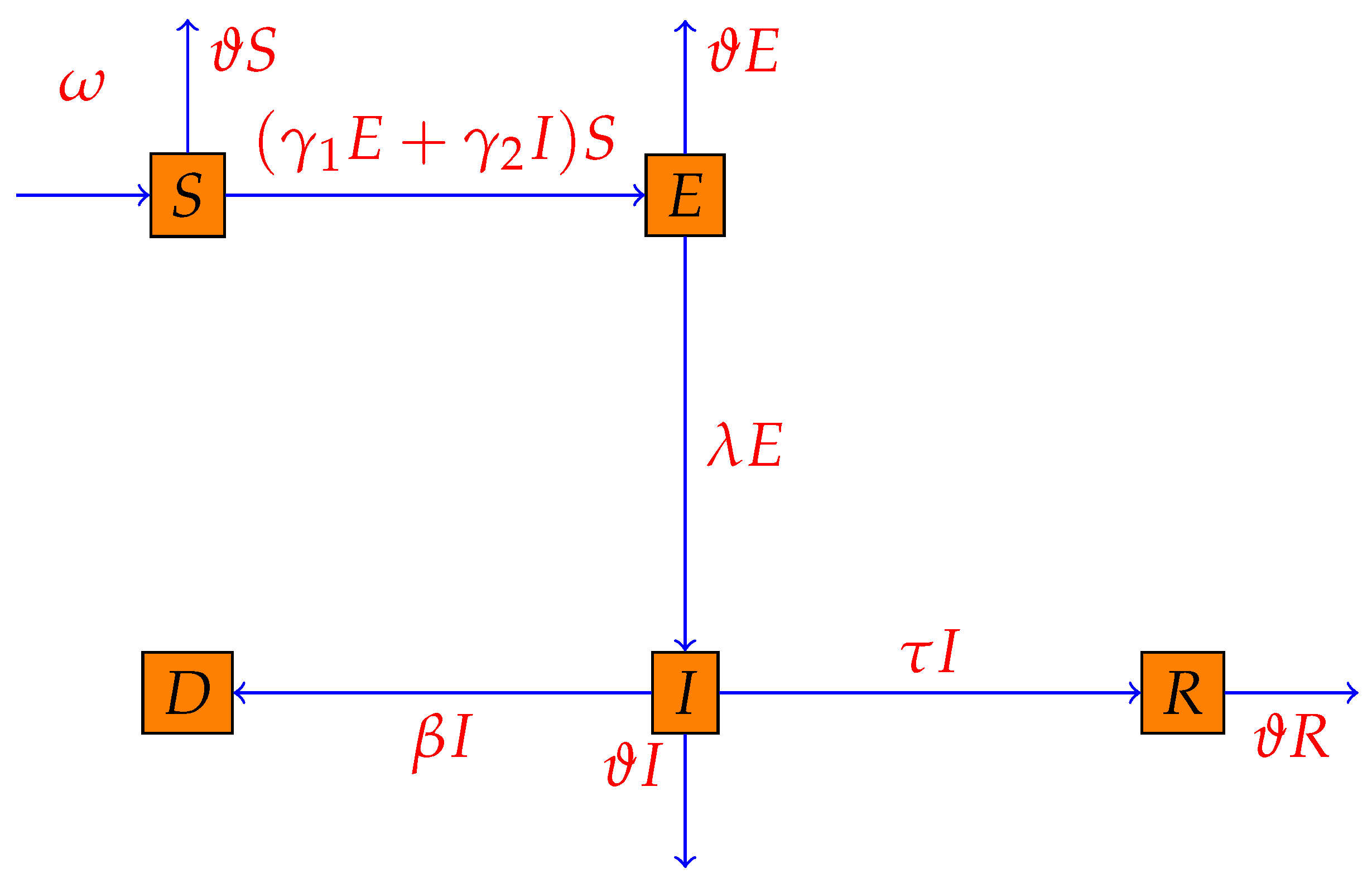
To design how to transfer COVID-19 between the target groups, We use the box model used in [30] and by adding another box to it, we arrive at an improved diagram as below:
The population in the classic SEIR model is considered constant, rendering it impossible to provide an accurate forecast using the model. To solve this problem, we have added the natural mortality rate ϑ and the natural birth rate ω to the diagram. We show the transmission rate of SARS-CoV-2 from asymptomatic infected people to susceptible people by γ 1 and the transmission rate from symptomatic infected people to susceptible people by γ 2 . After a few days, asymptomatic infected people become symptomatic and are transferred to category I at a rate of λ . People in group I are divided into three groups. One group recovers and is transferred to group R at a rate of τ , the next group dies with natural death at ϑ rate and the third group dies with COVID-19 disease and is transferred to category D at β rate.
Based on Figure 2 and the description provided, we adopt the following mathematical model
d S d t = ω ( γ 1 E ( t ) + γ 2 I ( t ) ) S ( t ) ϑ S ( t ) , d E d t = ( γ 1 E ( t ) + γ 2 I ( t ) ) S ( t ) ( λ + ϑ ) E ( t ) , d I d t = λ E ( t ) ( τ + ϑ + β ) I ( t ) , d R d t = τ I ( t ) ϑ R ( t ) , d D d t = β I ( t ) ,
where the initial conditions are S ( 0 ) , E ( 0 ) , I ( 0 ) , R ( 0 ) , D ( 0 ) , and all of them are nonnegative.
The spread of COVID-19 disease has a historical memory, and the infected people at any given time depends on the number of active cases in previous times. The integer-order derivative does not preserve the system’s historical memory, and thus is not suitable for modeling such epidemic diseases. The derivative with fractional-order maintains the internal memory and the historical memory of the system and therefore has a better performance in modeling the spread of diseases that have historical memory. The kernel of Caputo fractional derivative has no singularity and works very well in modeling natural phenomena, so we use this derivative for modeling.
In the above system, we use the Caputo fractional-order derivative κ , κ ( 0 , 1 ) instead of ordinary derivative. By changing the type of derivative, the equality of dimensions on both sides of the equations of system is disturbed, and we correct it using an auxiliary parameter δ , with sec. dimension (see [19]). Then, the fractional model for COVID-19 spread with Caputo derivative is presented by
δ κ 1 C D t κ S ( t ) = ω ( γ 1 E ( t ) + γ 2 I ( t ) ) S ( t ) ϑ S ( t ) , δ κ 1 C D t κ E ( t ) = ( γ 1 E ( t ) + γ 2 I ( t ) ) S ( t ) ( λ + ϑ ) E ( t ) , δ κ 1 C D t κ I ( t ) = λ E ( t ) ( τ + ϑ + β ) I ( t ) , δ κ 1 C D t κ R ( t ) = τ I ( t ) ϑ R ( t ) , δ κ 1 C D t κ D ( t ) = β I ( t ) ,
with initial conditions S ( 0 ) 0 , E ( 0 ) 0 , I ( 0 ) 0 , R ( 0 ) 0 , D ( 0 ) 0 .
In the following, we determine the region of non-negativity of solutions of the model and the boundedness of the solutions.

2.1. Feasibility Region

Let A = { ( S , E , I , R , D ) ( R 0 + ) 5 : D S + E + I + R ω ϑ } , the set A is feasibility region of the model (2).
Lemma 1. 
The set A is feasibility region of the model (2).
Proof. 
To show the non-negativity of solutions, we use the presented method in [15]. We can write
δ κ 1 C D 0 + κ S | S = 0 = ω 0 , δ κ 1 C D 0 + κ E | E = 0 = γ 2 I S 0 , δ κ 1 C D 0 + κ I | I = 0 = λ E 0 ,
δ κ 1 C D 0 + κ R | R = 0 = τ I 0 , δ κ 1 C D 0 + κ D | D = 0 = β I 0 ,
so all of them are nonnegative. We consider the auxiliary fractional-order differential system as follows
C D 0 + κ S ( t ) = δ 1 κ [ ω ( γ 1 E ( t ) + γ 2 I ( t ) ) S ( t ) ϑ S ( t ) ] + 1 υ , C D 0 + κ E ( t ) = δ 1 κ [ ( γ 1 E ( t ) + γ 2 I ( t ) ) S ( t ) ( λ + ϑ ) E ( t ) ] + 1 υ , C D 0 + κ I ( t ) = δ 1 κ [ λ E ( t ) ( τ + ϑ + β ) I ( t ) ] + 1 υ , C D 0 + κ R ( t ) = δ 1 κ [ τ I ( t ) ϑ R ( t ) ] + 1 υ , C D 0 + κ D ( t ) = δ 1 κ [ β I ( t ) ] + 1 υ ,
where υ N and initial values are S ( 0 ) = S 0 , E ( 0 ) = E 0 , I ( 0 ) = I 0 , R ( 0 ) = R 0 , D ( 0 ) = D 0 . We show that the solutions of system (3), ( S υ * ( t ) , E υ * ( t ) , I υ * ( t ) , R υ * ( t ) , D υ * ( t ) ) are nonnegative for t 0 . For this purpose, we assume that this is not the case. Thus, at some times t, the solutions are negative. Let
t m = inf { t > 0 | ( S υ * ( t ) , E υ * ( t ) , I υ * ( t ) , R υ * ( t ) , D υ * ( t ) ) ( R 0 + ) 5 } .
Then ( S υ * ( t m ) , E υ * ( t m ) , I υ * ( t m ) , R υ * ( t m ) , D υ * ( t m ) ( R 0 + ) 5 and one of the components is zero. Consider S υ * ( t m ) = 0 . On the other hand, we have
C D 0 + κ S υ * ( t m ) = δ 1 κ [ ω ( γ 1 E υ * ( t m ) + γ 2 I υ * ( t m ) ) S υ * ( t m ) ϑ S υ * ( t m ) ] + 1 υ > 0 ,
also from continuity of C D 0 + κ S υ * is results that C D 0 + κ S υ * ( [ t m , t m + υ ) ) R + for some υ > 0 . By Theorem (1), we conclude that S υ * ( [ t m , t m + υ ) ) R 0 + and so S υ * is nonnegative.
In a similar way, we can show that all of components E υ * , I υ * , R υ * , D υ * are nonnegative, and this is a contradiction. As υ , by Lemma (1) it is obtained that for all t 0 , ( S * , E * , I * , R * , D * ) ( R 0 + ) 5 . So we proved that all the solutions are non-negative.
We add the first four equations of the system (2), so
δ κ 1 C D t κ ( S + E + I + R ) = ω ϑ ( S + E + I + R ) β I ω ϑ ( S + E + I + R ) .
By applying the Laplace transform on both sides, we get
( S + E + I + R ) ( t ) = ( S + E + I + R ) ( 0 ) E κ ( ϑ δ 1 κ t κ ) + 0 t ω δ 1 κ η κ 1 E κ , κ ( ϑ δ 1 κ η κ ) d η ,
where S ( 0 ) , E ( 0 ) , I ( 0 ) , R ( 0 ) are the initial conditions. With a little simplification, we obtain
( S + E + I + R ) ( t ) = ( S + E + I + R ) ( 0 ) E κ ( ϑ δ 1 κ t κ ) + 0 t ω δ 1 κ η κ 1 i = 0 ( 1 ) i ϑ i δ i ( 1 κ ) η i κ Γ ( i κ + κ ) d η , = ω δ 1 κ ϑ δ 1 κ + E κ ( ϑ δ 1 κ t κ ) ( ( S + E + I + R ) ( 0 ) ω δ 1 κ ϑ δ 1 κ ) , = ω ϑ + E κ ( ϑ δ 1 κ t κ ) ( ( S + E + I + R ) ( 0 ) ω ϑ ) ,
so, if ( S + E + I + R ) ( 0 ) ω ϑ , then for t > 0 , ( S + E + I + R ) ( t ) ω ϑ .
Because D ( t ) S ( t ) + E ( t ) + I ( t ) + R ( t ) ω ϑ for all t 0 , so if D ( 0 ) A , then D ( t ) ω ϑ . Thus, the set A is feasibility region of the model (2). □

2.2. Reproduction Number and Equilibrium Points

In epidemics, two types of equilibrium points are defined. The first is the point at which there is no disease and is called the disease-free equilibrium point E 0 . Endemic equilibrium is a state in which the disease is not completely eradicated and there is still disease among the population. In this state, second equilibrium point as endemic equilibrium point E * is defined.
Given that the disease-free equilibrium point is a disease-free point, to find it we assume I = 0 , E = 0 , and then we set the other side of the equations of system (2) to zero and simplify the relations, thus the disease-free equilibrium point is obtained as E 0 = ( ω ϑ , 0 , 0 , 0 , N ω ϑ ) , N = S + E + I + R + D .
To determine the endemic equilibrium point of the system, we set the other side of the equations in system 2 to zero and form the following algebraic equations. Note, of course, that since D ( t ) does not exist in the first four equations, we do not consider the fifth equation here.
C D κ S ( t ) = C D κ E ( t ) = C D κ I ( t ) = C D κ R ( t ) = 0 .
By solving these equations, the endemic equilibrium point of the system is obtained as E * = ( S * , E * , I * , R * ) ,
S * = β ϑ + β λ + ϑ 2 + ϑ λ + ϑ τ + λ τ β γ 1 + γ 1 ϑ + γ 1 τ + λ γ 2 ,
E * = β γ 1 ω β ϑ 2 β ϑ λ + γ 1 ϑ ω + γ 1 ω τ ϑ 3 ϑ 2 λ ϑ 2 τ ϑ λ τ + λ ω γ 2 β γ 1 ϑ + β γ 1 λ + γ 1 ϑ 2 + γ 1 ϑ λ + γ 1 ϑ τ + γ 1 λ τ + ϑ λ γ 2 + λ 2 γ 2 ,
I * = { λ ( β γ 1 ω β ϑ 2 β ϑ λ + γ 1 ϑ ω + γ 1 ω τ ϑ 3 ϑ 2 λ ϑ 2 τ ϑ λ τ + λ ω γ 2 ) } /
{ β 2 γ 1 ( ϑ + λ ) + 2 β γ 1 ( ϑ 2 + ϑ λ + ϑ τ + λ τ ) + β γ 2 ( ϑ λ + λ 2 ) + γ 1 ( ϑ 3 + ϑ 2 λ + 2 ϑ 2 τ ) +
γ ϑ ( 2 λ τ + τ 2 ) + λ ( γ 1 τ 2 + ϑ 2 γ 2 ) + ϑ γ 2 ( λ 2 + λ τ ) + λ 2 γ 2 τ } ,
R * = { τ λ ( β γ 1 ω β ϑ 2 β ϑ λ + γ 1 ϑ ω + γ 1 ω τ ϑ 3 ϑ 2 λ ϑ 2 τ ϑ λ τ + λ ω γ 2 ) } /
{ ϑ ( β 2 γ ϑ + β 2 γ 1 λ + 2 β γ 1 ϑ 2 + 2 β γ 1 ϑ λ + 2 β γ 1 ϑ τ + 2 β γ 1 λ τ + β ϑ λ γ 2 + β λ 2 γ 2 + γ 1 ϑ 3
+ γ 1 ϑ 2 λ + 2 γ 1 ϑ 2 τ + 2 γ 1 ϑ λ τ + γ 1 ϑ τ 2 + γ 1 λ τ 2 + ϑ 2 λ γ 2 + ϑ λ 2 γ 2 + ϑ λ γ 2 τ + λ 2 γ 2 τ ) } .
Next, we calculate the basic reproduction number using the next-generation matrix method [37]. For this purpose, we consider the first four equations of System (2) in the following compact form
C D κ Ψ = F ( Ψ ) V ( Ψ ) ,
where
F ( Ψ ) = δ 1 κ + γ 1 S E + γ 2 S I 0 ,
and
V ( Ψ ) = δ 1 κ ( λ + ϑ ) E ( t ) λ E ( t ) + ( τ + ϑ + β ) I ( t ) .
The Jacobin matrix of F, V are obtained as
J F = δ 1 κ γ 1 S ( t ) γ 2 S ( t ) 0 0 , J v = δ 1 κ λ + ϑ 0 λ τ + ϑ + β
By placing the disease-free equilibrium point value in the resulting matrices, so we have
F = J F ( E 0 ) = δ 1 κ γ 1 ω ϑ γ 2 ω ϑ 0 0 , V = J v ( E 0 ) = δ 1 κ λ + ϑ 0 λ τ + ϑ + β
The next generation matrix for system (1) is defined as F V 1 so that
F V 1 = δ 2 2 κ γ 1 ω ϑ γ 2 ω ϑ 0 0 1 λ + ϑ 0 λ ( λ + ϑ ) ( τ + ϑ + β ) 1 τ + ϑ + β = δ 2 2 κ γ 1 ω ( τ + ϑ + β ) + γ 2 ω λ ϑ ( λ + ϑ ) ( τ + ϑ + β ) γ 2 ω ϑ ( τ + ϑ + β ) 0 0
Considering the largest eigenvalue of matrix F V 1 as a basic reproduction number R 0 = ρ ( F V 1 ) , we have
R 0 = γ 1 ω ( τ + ϑ + β ) + γ 2 ω λ ϑ ( λ + ϑ ) ( τ + ϑ + β ) .
In epidemiological discussions, the reproduction number is used as an important factor in the investigate of transmission and continuation of infectious diseases outbreak.

2.3. Stability of Equilibrium Point

We use the Jacobin matrix to determine the stability conditions of the equilibrium point. The Jacobin matrix of differential system (2) is defined as follows:
J = δ 1 κ ( γ 1 E + γ 2 I ) ϑ γ 1 S γ 2 S 0 0 γ 1 E + γ 2 I γ 1 S ( λ + ϑ ) γ 2 S 0 0 0 λ ( τ + ϑ + β ) 0 0 0 0 τ ϑ 0 0 0 β 0 0 .
By placing the disease-free equilibrium point coordinates E 0 in the Jacobin matrix, resulting in the following matrix
J = δ 1 κ ϑ γ 1 ω ϑ γ 2 ω ϑ 0 0 0 γ 1 ω ϑ ( λ + ϑ ) γ 2 ω ϑ 0 0 0 λ ( τ + ϑ + β ) 0 0 0 0 τ ϑ 0 0 0 β 0 0 .
One type of stability is marginal stability, which is defined below.
Definition 1. 
If all the poles on the imaginary axis are distinct and all the remaining poles have negative real parts, the system is called marginally stable.
According to this definition, we consider the following theorem:
Theorem 1. 
If R 0 < 1 , then the disease-free equilibrium point E 0 of system (1) is marginal stable.
Proof. 
By calculating the characteristic equation of J ( E 0 ) , d e t ( μ I J ( E 0 ) ) = 0 , we obtain
μ ( μ + ϑ ) 2 = 0 ,
μ 2 + μ ( ( τ + ϑ + β ) ( γ 1 ω ϑ ( λ + ϑ ) ) ) ( τ + ϑ + β ) ( γ 1 ω ϑ ( λ + ϑ ) ) λ γ 2 ω ϑ = 0 .
By solving the above equations we get μ 1 = 0 , μ 2 = ϑ . To determine the sign of the real part of the roots of last equation, we consider b 0 = 1 , b 1 = ( τ + ϑ + β ) ( γ 1 ω ϑ ( λ + ϑ ) ) , b 2 = ( τ + ϑ + β ) ( γ 1 ω ϑ ( λ + ϑ ) ) λ γ 2 ω ϑ = 0 . Therefore, the equation is written as
b 0 μ 2 + b 1 μ + b 2 = 0 .
Now, if R 0 < 1 , we get
γ 1 ω ( τ + ϑ + β ) + γ 2 ω λ ϑ ( λ + ϑ ) ( τ + ϑ + β ) < 1 γ 1 ω ϑ ( τ + ϑ + β ) + γ 2 ω λ ϑ ( λ + ϑ ) ( τ + ϑ + β ) < 0 ,
( τ + ϑ + β ) ( γ 1 ω ϑ ( λ + ϑ ) ) + γ 2 ω λ ϑ > 0 b 2 > 0 .
On the other hand, we have
R 0 < 1 γ 1 ω ϑ ( τ + ϑ + β ) + γ 2 ω λ ϑ < ( λ + ϑ ) ( τ + ϑ + β ) ,
γ 1 ω ϑ ( τ + ϑ + β ) < ( λ + ϑ ) ( τ + ϑ + β ) γ 1 ω ϑ < ( λ + ϑ ) ,
γ 1 ω ϑ ( λ + ϑ ) < 0 , b 1 > 0 .
It has been shown that b 1 > 0 , b 2 > 0 , so by the Routh–Hurwitz criteria, we can conclude that the roots of equation are negative. Thus, the disease-free equilibrium point E 0 of system (1) is marginally stable. It should be noted that in examining the stability conditions of the equilibrium point, the method of Matignon theorem (see, [38,39]) can also be used, which we encourage young researchers to re-examine the stability conditions using this method. □

3. Existence and Uniqueness of Solution

Fixed-point theorems are one of the most powerful methods in the nonlinear systems to prove the existence of solution. In the present section, we first convert the differential equations system (2) to a system of integral equations, then show that the kernels of these integrals hold the Lipschitz condition, and finally we show that the system has a unique solution by one of the fixed-point theorems. For this end, we consider model (2) as following compact form
δ κ 1 C D t κ S ( t ) = Z 1 ( t , S ( t ) ) , δ κ 1 C D t κ E ( t ) = Z 2 ( t , E ( t ) ) , δ κ 1 C D t κ I ( t ) = Z 3 ( t , I ( t ) ) , δ κ 1 C D t κ R ( t ) = Z 4 ( t , R ( t ) ) , δ κ 1 C D t κ D ( t ) = Z 5 ( t , D ( t ) ) .
Now we take integrals from the sides of the above system,
S ( t ) S ( 0 ) = δ 1 κ Γ ( κ ) 0 t Z 1 ( ξ , S ) ( t ξ ) κ 1 d ξ , E ( t ) E ( 0 ) = δ 1 κ Γ ( κ ) 0 t Z 2 ( ξ , E ) ( t ξ ) κ 1 d ξ , I ( t ) I ( 0 ) = δ 1 κ Γ ( κ ) 0 t Z 3 ( ξ , I ) ( t ξ ) κ 1 d ξ , R ( t ) R ( 0 ) = δ 1 κ Γ ( κ ) 0 t Z 4 ( ξ , R ) ( t ξ ) κ 1 d ξ , D ( t ) D ( 0 ) = δ 1 κ Γ ( κ ) 0 t Z 5 ( ξ , D ) ( t ξ ) κ 1 d ξ .
Next, we determine the necessary conditions for establishing Lipschitz condition for kernels Z n , n = 1 , 2 , 3 , 4 , 5 .
Theorem 2. 
The Lipschitz condition and contraction are satisfied for kernel Z 1 , whenever we have
0 γ 1 u 2 + γ 2 u 3 + ϑ < 1 .
Proof. 
We consider the value of Z 1 for S and S 1 as follows
Z 1 ( t , S ) Z 1 ( t , S 1 ) = ( γ 1 E ( t ) + γ 2 I ( t ) ) ( S ( t ) S 1 ( t ) ) ϑ ( S ( t ) S 1 ( t ) ) , γ 1 E ( t ) + γ 2 I ( t ) S ( t ) S 1 ( t ) + ϑ S ( t ) S 1 ( t ) , ( γ 1 E ( t ) + γ 2 I ( t ) ) + ϑ ) S ( t ) S 1 ( t ) , ( γ 1 u 2 + γ 2 u 3 + ϑ ) S ( t ) S 1 ( t ) .
Let w 1 = γ 1 u 2 + γ 2 u 3 + ϑ , where E , I are bounded functions and E ( t ) u 2 , I ( t ) u 3 . Then
Z 1 ( t , S ) Z 1 ( t , S 1 ) w 1 ( S ( t ) S 1 ( t ) ) .
So the Lipschitz condition and contraction is obtained for Z 1 ( t ) . □
Similarly, the other kernels Z n , n = 2 , 3 , 4 , 5 can be proved to satisfy the Lipschitz condition,
Z 2 ( t , E ) Z 2 ( t , E 1 ) w 2 ( E ( t ) E 1 ( t ) ) , Z 3 ( t , I ) Z 3 ( t , I 1 ) w 3 ( I ( t ) I 1 ( t ) ) , Z 4 ( t , R ) Z 4 ( t , R 1 ) w 4 ( R ( t ) R 1 ( t ) ) , Z 5 ( t , D ) Z 5 ( t , D 1 ) w 5 ( D ( t ) D 1 ( t ) ) ,
where S ( t ) u 1 , and w 2 = γ 1 u 1 + λ + ϑ , w 3 = τ + ϑ + β , w 4 = ϑ , w 5 = 0 are bounded functions. So if 0 w n < 1 , n = 2 , 3 , 4 , 5 then kernels Z n , n = 2 , 3 , 4 , 5 are contraction.
We consider the following recursive forms according to System (4),
Λ 1 n ( t ) = S n ( t ) S n 1 ( t ) = δ 1 κ Γ ( κ ) 0 t ( Z 1 ( ξ , S n 1 ) Z 1 ( ξ , S n 2 ) ) ( t ξ ) κ 1 d ξ ,
Λ 2 n ( t ) = E n ( t ) E n 1 ( t ) = δ 1 κ Γ ( κ ) 0 t ( Z 2 ( ξ , E n 1 ) Z 2 ( ξ , E n 2 ) ) ( t ξ ) κ 1 d ξ ,
Λ 3 n ( t ) = I n ( t ) I n 1 ( t ) = δ 1 κ Γ ( κ ) 0 t ( Z 3 ( ξ , I n 1 ) Z 3 ( ξ , I n 2 ) ) ( t ξ ) κ 1 d ξ ,
Λ 4 n ( t ) = R n ( t ) R n 1 ( t ) = δ 1 κ Γ ( κ ) 0 t ( Z 4 ( ξ , R n 1 ) Z 4 ( ξ , R n 2 ) ) ( t ξ ) κ 1 d ξ ,
Λ 5 n ( t ) = D n ( t ) D n 1 ( t ) = δ 1 κ Γ ( κ ) 0 t ( Z 4 ( ξ , D n 1 ) Z 5 ( ξ , D n 2 ) ) ( t ξ ) κ 1 d ξ .
The norm of Λ 1 n ( t ) is obtained as follows
Λ 1 n ( t ) = S n ( t ) S n 1 ( t ) , = δ 1 κ Γ ( κ ) 0 t ( Z 1 ( ξ , S n 1 ) Z 1 ( ξ , S n 2 ) ) ( t ξ ) κ 1 d ξ , δ 1 κ Γ ( κ ) 0 t Z 1 ( ξ , S n 1 ) Z 1 ( ξ , S n 2 ) ) ( t ξ ) ξ 1 d ξ ,
condition (5) results
Λ 1 n ( t )     δ 1 κ Γ ( κ ) w 1 0 t Λ 1 ( n 1 ) ( t ) ( ξ ) d ξ .
For Λ i n ( t ) , i = 2 , 3 , 4 , 5 can also be shown that
Λ 2 n ( t )     δ 1 κ Γ ( κ ) w 2 0 t Λ 2 ( n 1 ) ( t ) ( ξ ) d ξ ,
Λ 3 n ( t )     δ 1 κ Γ ( κ ) w 3 0 t Λ 3 ( n 1 ) ( t ) ( ξ ) d ξ ,
Λ 4 n ( t )     δ 1 κ Γ ( κ ) w 4 0 t Λ 4 ( n 1 ) ( t ) ( ξ ) d ξ ,
Λ 5 n ( t )     δ 1 κ Γ ( κ ) w 5 0 t Λ 5 ( n 1 ) ( t ) ( ξ ) d ξ .
According to the results, we obtain
S n ( t ) = m = 1 n Λ 1 m ( t ) , E n ( t ) = m = 1 n Λ 2 m ( t ) , I n ( t ) = m = 1 n Λ 3 m ( t ) ,
R n ( t ) = m = 1 n Λ 4 m ( t ) , D n ( t ) = m = 1 n Λ 5 m ( t ) .
Theorem 3. 
There exists a solution for fractional model (2), if there exists t 1 such that
δ 1 κ Γ ( κ ) t 1 w n < 1 .
Proof. 
Using Equations (6) and (7) and recursive equations, We conclude that
Λ 1 n ( t )     S n ( 0 ) [ δ 1 κ Γ ( κ ) w 1 t ] n ,
Λ 2 n ( t )     E n ( 0 ) [ δ 1 κ Γ ( κ ) w 2 t ] n ,
Λ 3 n ( t )     I n ( 0 ) [ δ 1 κ Γ ( κ ) w 3 t ] n ,
Λ 4 n ( t )     R n ( 0 ) [ δ 1 κ Γ ( κ ) w 4 t ] n ,
Λ 5 n ( t )     D n ( 0 ) [ δ 1 κ Γ ( κ ) w 5 t ] n .
Now to show that the model (2) solution constructs by the above continuous functions, we suppose that
S ( t ) S ( 0 ) = S n ( t ) Y 1 n ( t ) ,
E ( t ) E ( 0 ) = E n ( t ) Y 2 n ( t ) ,
I ( t ) I ( 0 ) = I n ( t ) Y 3 n ( t ) ,
R ( t ) R ( 0 ) = R n ( t ) Y 4 n ( t ) ,
D ( t ) D ( 0 ) = D n ( t ) Y 5 n ( t ) ,
then
Y 1 n ( t ) = δ 1 κ Γ ( κ ) 0 t ( Z 1 ( ξ , S ) Z 1 ( ξ , S n 1 ) ) d ξ , δ 1 κ Γ ( κ ) 0 t Z 1 ( ξ , S ) Z 1 ( ξ , S n 1 ) d ξ , δ 1 κ Γ ( κ ) w 1 S S n 1 t .
If we continue the same repetitive method, we will get the results
Y 1 n ( t )   [ δ 1 κ Γ ( κ ) t ] n + 1 w 1 n + 1 k .
At t 1 , we obtain
Y 1 n ( t )   [ δ 1 κ Γ ( κ ) t 1 ] n + 1 w 1 n + 1 b .
If n , we obtain Y 1 n ( t ) 0 . It can be similarly shown that Y i n ( t ) 0 , i = 2 , 3 , 4 , 5 . This completes the proof. □
To show the uniqueness of system solution, we consider that there is a another solution for a system such as ( S 1 , E 1 , I 1 , R 1 , D 1 ) . So, we can write
S ( t ) S 1 ( t ) = δ 1 κ Γ ( κ ) 0 t ( Z 1 ( ξ , S ) Z 1 ( ξ , S 1 ) ) d ξ .
The norm of the recent equation is
S ( t ) S 1 ( t )   = δ 1 κ Γ ( κ ) 0 t Z 1 ( ξ , S ) Z 1 ( ξ , S 1 ) d ξ .
From condition (5), we obtain
S ( t ) S 1 ( t )   δ 1 κ Γ ( κ ) w 1 t S ( t ) S 1 ( t ) .
We conclude
S ( t ) S 1 ( t ) ( 1 δ 1 κ Γ ( κ ) w 1 t ) 0 .
Theorem 4. 
In order for the solution of the system (2) to be unique, the following condition must be met
1 δ 1 κ Γ ( κ ) w 1 t > 0 .
Proof. 
Equation (8) shows that
S ( t ) S 1 ( t ) ( 1 δ 1 κ Γ ( κ ) w 1 t ) 0 .
We conclude from this relation and condition of theorem that S ( t ) S 1 ( t )   = 0 . Then S ( t ) = S 1 ( t ) . The same relations can be proved for E , I , R , D . □

4. Numerical Analysis

To find the approximate solution of fractional-order system of the model (2), we use the Euler method for the fractional-order system ([40]). Furthermore, we present a numerical simulation for the COVID-19 outbreak in the world.

4.1. Numerical Method

To solve the fractional system (2) using the Euler method, we first write the system in the following form
δ κ 1 C D t κ ϖ ( t ) = b ( t , ϖ ( t ) ) , ϖ ( 0 ) = ϖ 0 , 0 t T < ,
so that ϖ = ( S , E , I , R , D ) R + 5 , and the initial value of the vector is ϖ 0 = ( S 0 , E 0 , I 0 , R 0 , D 0 ) . Furthermore, the continuous vector function b ( t ) R is satisfied in the following Lipschitz condition
b ( ϖ 1 ( t ) ) b ( ϖ 2 ( t ) )   ϵ ϖ 1 ( t ) ϖ 2 ( t ) , ϵ > 0 .
By integrating from Equation (9), we conclude
ϖ ( t ) = δ 1 κ [ ϖ 0 + I κ b ( ϖ ( t ) ) ] , 0 t T < .
Suppose that e = T 0 N and t n = n e , t [ 0 , T ] and n = 0 , 1 , 2 , . . . , N . We consider the approximation of ϖ ( t ) at t = t n as ϖ n . Using the Euler method ([40]) on last equation, we have
ϖ n + 1 = δ 1 κ [ ϖ 0 + e κ Γ ( κ + 1 ) h = 0 n y n + 1 , h b ( t h , ϖ h ) ] , h = 0 , 1 , 2 , . . . , N 1 ,
so that
y n + 1 , h = ( n + 1 h ) κ ( n h ) κ , h = 0 , 1 , 2 , . . . , n .
Now, if we put each of the functions S , E , I , R , D in Equation (9) instead of Function ϖ ( t ) , then using Equation (9), the approximate solutions for each of the functions S , E , I , R , D are obtained as follows.
S ( n + 1 ) = δ 1 κ [ S 0 + e κ Γ ( κ + 1 ) h = 0 n y n + 1 , h d 1 ( t h , ϖ h ) ] ,
E ( n + 1 ) = δ 1 κ [ E 0 + e κ Γ ( κ + 1 ) h = 0 n y n + 1 , h d 2 ( t h , ϖ h ) ] ,
I ( n + 1 ) = δ 1 κ [ I 0 + e κ Γ ( κ + 1 ) h = 0 n y n + 1 , h d 3 ( t h , ϖ h ) ] ,
R ( n + 1 ) = δ 1 κ [ R 0 + e κ Γ ( κ + 1 ) h = 0 n y n + 1 , h d 4 ( t h , ϖ h ) ] ,
D ( n + 1 ) = δ 1 κ [ D 0 + e κ Γ ( κ + 1 ) h = 0 n y n + 1 , h d 5 ( t h , ϖ h ) ] ,
so that y n + 1 , h = ( n + 1 h ) κ ( n h ) κ , d 1 ( t , ϖ ( t ) ) = ω ( γ 1 E ( t ) + γ 2 I ( t ) ) S ( t ) ϑ S ( t ) , d 2 ( t , ϖ ( t ) ) = ( γ 1 E ( t ) + γ 2 I ( t ) ) S ( t ) ( λ + ϑ ) E ( t ) , d 3 ( t , ϖ ( t ) ) = λ E ( t ) ( τ + ϑ + β ) I ( t ) , d 4 ( t , ϖ ( t ) ) = τ I ( t ) ϑ R ( t ) , d 5 ( t , ϖ ( t ) ) = β I ( t ) .

4.2. Numerical Simulation

To date, several waves of COVID-19 outbreak have occurred across the world, and due to the identification of various mutations in the coronavirus, a new wave has started from 22 June 2021, and the number of infected people is increasing. We numerically simulate the recent wave of COVID-19 spread around the world and provide a numerical prediction for the continued spread of the disease worldwide.
According to the World Health Organization, in 2021 the birth rate and natural mortality in the world were reported to be n = 17.873 and b = 7.645 per 1000 people, respectively. According to the report of the Worldometer website, we consider the world population as 7,888,599,433 in 2021. So, the daily birth rate will be ω = n × N 365 × 1000 = 386282 and the daily death rate will be ϑ = b 365 × 1000 = 0.0000209 . According to a report published on the Worldometer website, on 22 June, the number of actively infected people and the number of recovered people and the number of people who died with COVID-19 are I ( 0 ) = 11236813 , R ( 0 ) = 164763002 and D ( 0 ) = 3914791 , respectively. The world’s population in 2021 was about 7,888,599,433 people, which if we consider the number of asymptomatic people is E ( 0 ) = 1000000 , the number of susceptible people at the beginning of the wave will be S ( 0 ) = 7707684827 . From 22 June to 24 August, the total number of deaths was 549,203 and the total number of infected people was 34301737, and based on this, we consider the death rate due to COVID-19 in this wave β = 549203 34301737 = 0.016 . The recovery period is between 10 and 20 days (see [41]), we consider the recovery time of infected people with an average of 11 days and obtain τ = 0.1093 . By the fitting data method and Matlab software and based on the data reported for the number of infected people with COVID-19 by the World Health Organization from June 22 to August 24, we obtain the other parameters as follows λ = 0.24 , γ 1 = 5.6 × 10 13 and γ 2 = 1.9 × 10 11 .
Figure 3 shows the result of model (2) for infected people I ( t ) in the recent wave with fractional order κ = 0.996 with real data. We see that the fractional-order model follows the real data well. This figure also shows that if the situation continues like this and no special measures are taken, it will take several months to cross the wave peak and the number of actively infected people can increase to 80 million people. These results show that the World Health Organization should try to make the necessary vaccine available to all countries and accelerate the vaccination process so that the results of the simulation do not happen.
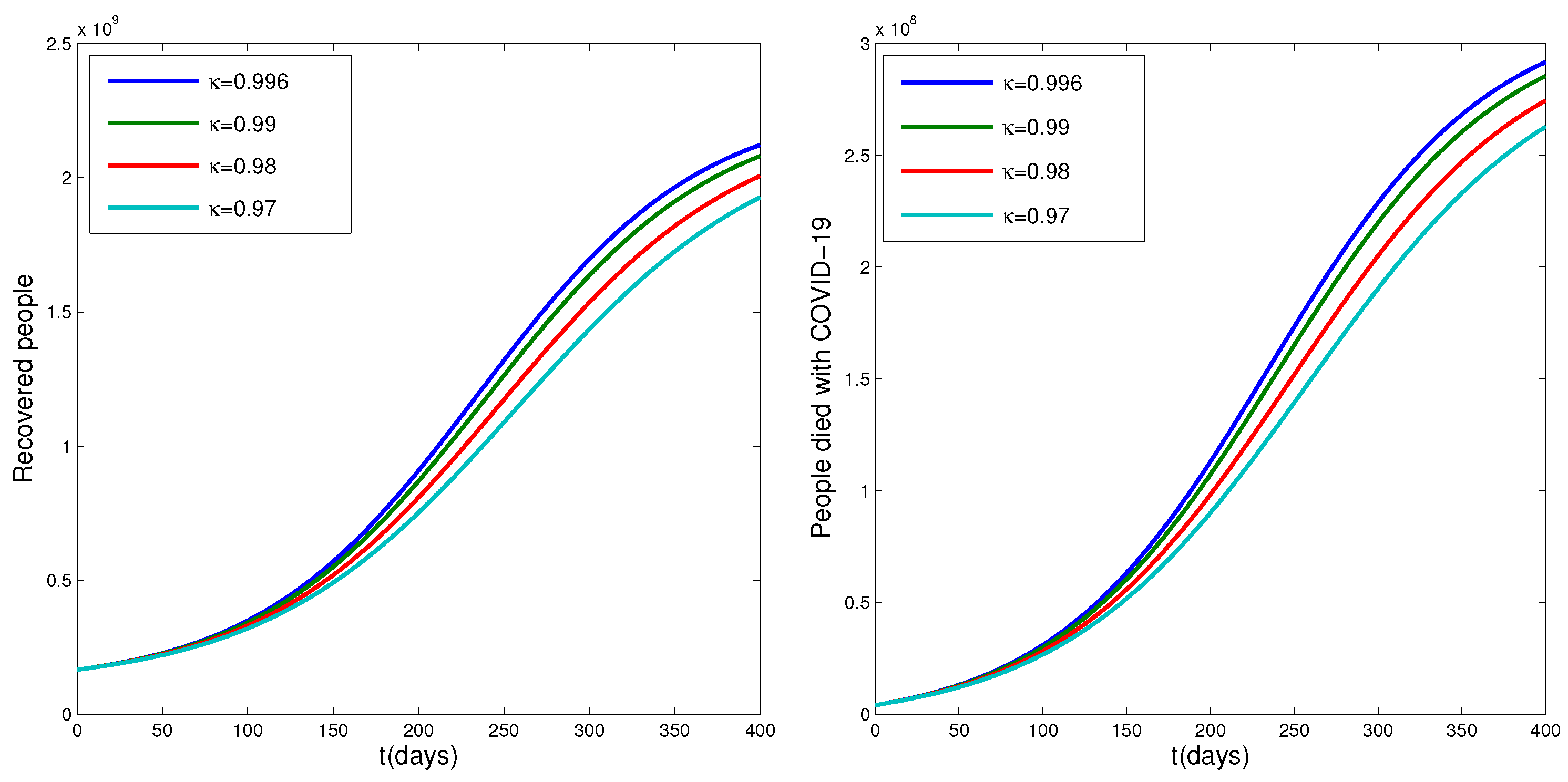
In Figure 4 and Figure 5, the results of the model are plotted for the other four groups and show that the number of susceptible people decreases and the number of infected and recovered and dead people increase. Furthermore, to investigate the effect of the order of derivation on the results, we plot the results for several different fractional orders, and we see that the results have the same behaviour but the obtained numerical value is different for them. The influence of the order of derivation in the obtained numerical results clearly shows the importance of determining the appropriate fractional order for the virus spread model.
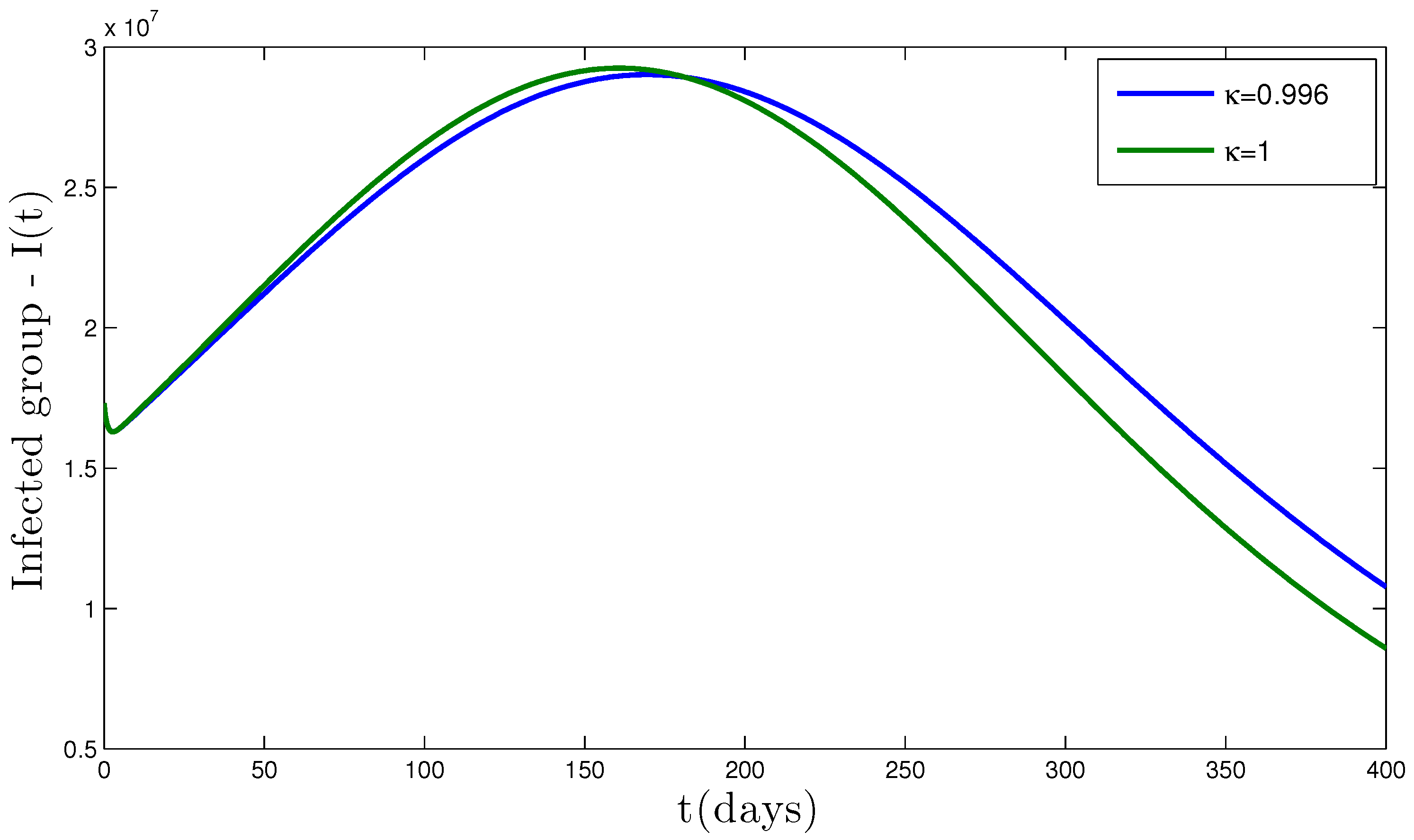
For further comparison, we have drawn the numerical results of the fractional-order and ordinary-order models in Figure 6, and the plot shows that the results are very different in the long run.
Based on the data obtained for this wave COVID-19 outbreak, the basic reproduction number is obtained as R 0 = 2.84 , which indicates that the disease has not yet emerged from the epidemic state and that each infected person infects more than one person, and this poses a serious threat to all countries. Therefore, there will be a need to accelerate vaccination in all countries.
In Table 1 and Table 2, we compare the real data reported for the number of infected people and the results of the model for I ( t ) with three types of fractional-order derivatives. The tables show that the results of the fractional-order model with the Caputo fractional derivative with order κ = 0.996 have less errors than the other two types of derivative, the Caputo–Fabrizio derivative and the Atangana–Baleanu derivative.

4.3. Sensitivity of R 0 with Respect to Model Parameters

According to the formula of number of reproduction, each of the parameters of the model affects it.To calculate the impact of each parameter, we use the formula used in [42], which calculates the impact of each parameter as a numerical value.
Given the importance of the COVID-19 outbreak globally, using the parameters of the third wave of COVID-19 spread in the world, we obtain
S γ 1 = R 0 γ 1 γ 1 R 0 = ω ( τ + ϑ + β ) γ 1 ω ( τ + ϑ + β ) + γ 2 ω λ = 2.71 × 10 10 > 0 ,
S ω = R 0 ω ω R 0 = 1 > 0 ,
S λ = R 0 λ λ R 0 = ( γ 2 ϑ ω γ 1 ω ( τ + ϑ + β ) ) λ ( λ + ϑ ) ( γ 1 ω ( τ + ϑ + β ) + γ 2 ω λ ) = 1.51 × 10 2 < 0 ,
S γ 2 = R 0 γ 2 γ 2 R 0 = λ γ 2 γ 1 ( τ + ϑ + β ) + γ 2 λ = 0.985 > 0 ,
S τ = R 0 τ τ R 0 = τ [ γ 1 ω ( τ + ϑ + β ) 1 ] ( τ + ϑ + β ) [ γ 1 ω ( τ + ϑ + β ) + γ 2 ω λ ] = 4.88 × 10 5 < 0 ,
S β = R 0 β β R 0 = β λ γ 2 ( τ + ϑ + β ) [ γ 1 ( τ + ϑ + β ) + γ 2 λ ] = 1.26 × 10 1 < 0 ,
S ϑ = R 0 ϑ ϑ R 0 = γ 1 ω γ 1 ω ( τ + ϑ + β ) + γ 2 ω λ ϑ λ + ϑ ϑ τ + ϑ + β 1 = 0.879 < 0 .
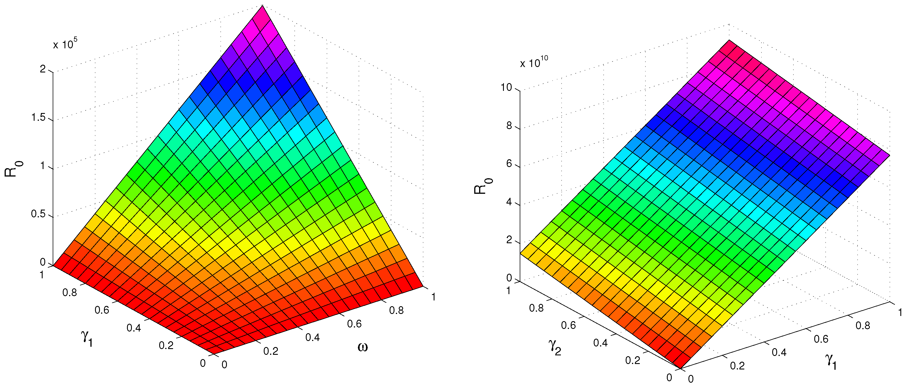
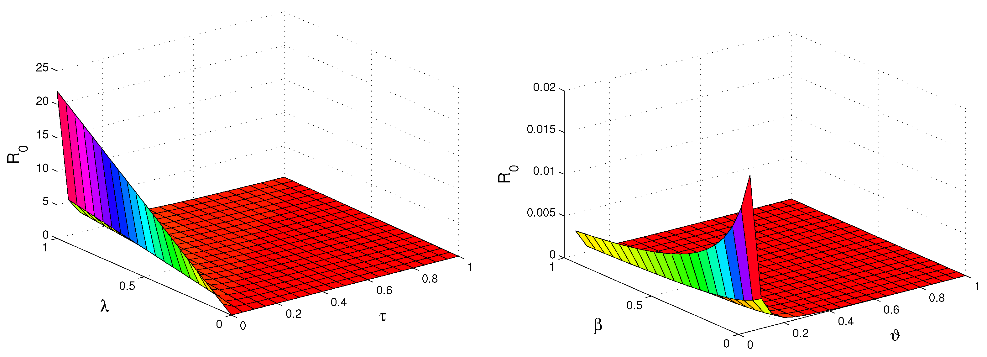
The R 0 sensitivity with respect to each of the parameters of Model (2) has been shown in Figure 7, Figure 8 and Figure 9. Figure 7 shows that parameters ω , γ 1 and γ 2 have a direct effect on R 0 , so that by increasing them, the value of R 0 increases, and among them, γ 1 has the greatest effect on R 0 . Figure 8 and Figure 9 show that λ , τ , β and ϑ have a negative effect on the value of R 0 , so that as they increase, the value of R 0 decreases, and among them, τ has the most negative effect on R 0 . Accordingly, in order to reducing the amount of R 0 and controlling the COVID-19 spread, the amount of γ 1 and γ 2 should be reduced through social distancing and quarantine of infected people.

5. Discussion and Conclusions

In this study, the application of a box fractional-order model integrated with a Caputo fractional derivative was investigated for COVID-19 outbreak. The study was extended to inspect the solutions boundedness and non-negativity. The existence of a unique answer for the system was proved by using the fixed-point theory. The equilibrium points of the system were computed and the stability conditions of the disease-free equilibrium point were determined. Next, with the fractional Euler method, the approximate answers of the system were determined and a numerical simulation for the recent wave of global COVID-19 spread was performed. In the recent wave, the basic reproduction number is obtained as R 0 = 2.84 > 1 , which indicates that the release of COVID-19 will continue for the time being and has not left the pandemic state. The simulation results have also shown that this wave will last for several months and the number of people actively infected could increase to 80 million, a statistic that places many countries in a critical situation. The number of people who are dying with COVID-19 is also increasing dramatically, and to prevent this situation, the vaccination process should be accelerated and the vaccine should be made available to all countries.
The results of the model were also calculated by using three types of fractional-order derivatives of Caputo, Caputo–Fabrizio and Atangana–Baleanu. They were subsequently compared in two tables of results with real data. We observed that the results of the Caputo fractional-order derivative are more consistent with the real data.
Based on the consideration of the significance of the reproduction number in determining the disease propagation process, the effect of each model parameter on the R 0 was investigated via numerical simulation. The subsequent results show that the rate of disease transmission from infected to susceptible individuals still has a large effect on R 0 . Social isolation and the quarantining of infected people also have the greatest impact on controlling the spread of the disease.
Young researchers can evaluate the effect of each control by placing different controls on the system and calculating the optimal control and simulating the results. However, we could not check the Enter system control in this article, since we did not have access to real data related to the applied controls such as vaccination.

Author Contributions

Data curation, formal analysis, conceptualization, methodology, software, writing—original draft, R.Y., A.J. and S.A.-A.; conceptualization, R.Y., A.J. and S.A.-A.; methodology, writing, review and editing, R.Y., A.J. and S.A.-A.; visualization, R.Y.; investigation, R.Y., A.J. and S.A.-A.; project administration, R.Y.; funding acquisition, R.Y., A.J. and S.A.-A. All authors have read and agreed to the published version of the manuscript.

Funding

This research received no external funding.

Data Availability Statement

Data can be provided upon request from the authors.

Conflicts of Interest

The authors declare no conflict of interest.

References

  1. Wang, Y.; Sun, H.; Wei, J.; Liu, X.; Liu, T.; Fan, Y. A mathematical model of human heart including the effects of heart contractility varying with heart rate changes. J. Biomech. 2018, 25, 129–137. [Google Scholar] [CrossRef]
  2. Ghalavand, Y.; Rahimi, A.; Hatamipour, M.S. Mathematical modeling for humidifier performance in a compression desalination system: Insulation effects. Desalination 2018, 433, 48–55. [Google Scholar] [CrossRef]
  3. Xu, H.; Chen, B.; Tan, P.; Cai, W.; He, W.; Farrusseng, D.; Ni, M. Modeling of all porous solid oxide fuel cells. Appl. Energy 2018, 219, 105–113. [Google Scholar] [CrossRef]
  4. Aleisaa, E.; Al-Shayji, K. Ecological–economic modeling to optimize a desalination policy: Case study of an arid rentier state. Desalination 2018, 430, 64–73. [Google Scholar] [CrossRef]
  5. Shi, Y.; Wang, Y.; Cai, M.; Zhang, B.; Zhu, J. An aviation oxygen supply system based on a mechanical ventilation model. Chin. J. Aeronaut. 2018, 31, 197–204. [Google Scholar] [CrossRef]
  6. Zurman, A.; Sarmoria, C.; Brandolin, A.; Asteasuain, M. Mathematical modeling of reverse atom transfer radical polymerization in miniemulsion. Comput. Mater. Sci. 2018, 145, 48–59. [Google Scholar] [CrossRef]
  7. Jagirdar, M.; Lee, P.S. Mathematical modeling and performance evaluation of a desiccant coated fin-tube heat exchanger. Appl. Energy 2018, 212, 401–415. [Google Scholar] [CrossRef]
  8. Kosmidis, K.; Macheras, P. A fractal kinetics SI model can explain the dynamics of COVID-19 epidemics. PLoS ONE 2020, 15, e0237304. [Google Scholar] [CrossRef] [PubMed]
  9. Cooper, I.; Mondal, A.; Antonopoulos, C.G. A SIR model assumption for the spread of COVID-19 in different communities. Chaos Solitons Fractals 2020, 139, 110057. [Google Scholar] [CrossRef]
  10. Martínez, V. A Modified SIRD Model to Study the Evolution of the COVID-19 Pandemic in Spain. Symmetry 2021, 13, 723. [Google Scholar] [CrossRef]
  11. Youssef, H.M.; Alghamdi, N.A.; Ezzat, M.A.; El-Bary, A.A.; Shawky, M.A. A modified SEIR model applied to the data of COVID-19 spread in Saudi Arabia. AIP Adv. 2020, 10, 125210. [Google Scholar] [CrossRef] [PubMed]
  12. Lopez, L.; Rodo, X. A modified SEIR model to predict the COVID-19 outbreak in Spain and Italy: Simulating control scenarios and multi-scale epidemics. Results Phys. 2021, 21, 103746. [Google Scholar] [CrossRef] [PubMed]
  13. Groendyke, C.; Combs, A. Modifying the network-based stochastic SEIR model to account for quarantine: An application to COVID-19. Epidemiol. Methods 2021, 10, 20200030. [Google Scholar] [CrossRef]
  14. Khedher, N.B.; Kolsi, L.; Alsaifd, H. A multi-stage SEIR model to predict the potential of a new COVID-19 wave in KSA after lifting all travel restrictions. Alex. Eng. J. 2021, 60, 3965–3974. [Google Scholar] [CrossRef]
  15. Almeida, R.; Cruz, A.M.C.B.; Martins, N.; Monteiro, M.T.T. An epidemiologial MSEIR model described by the Caputo frational derivative. Int. J. Dynam. Control. 2019, 7, 776–784. [Google Scholar] [CrossRef] [Green Version]
  16. Koca, I. Analysis of rubella disease model with non-local and non-singular fractional derivatives. J. Theor. Appl. 2018, 8, 17–25. [Google Scholar] [CrossRef] [Green Version]
  17. Khan, M.A.; Hammouch, Z.; Baleanu, D. Modeling the dynamics of hepatitis B via the Caputo-Fabrizio derivative. Math. Model. Nat. Phenom. 2019, 14, 311. [Google Scholar] [CrossRef]
  18. Singh, J. Analysis of fractional blood alcohol model with composite fractional derivative. Chaos Solitons Andfractals 2020, 140, 110127. [Google Scholar] [CrossRef]
  19. Ullah, M.Z.; Alzahrani, A.K.; Baleanu, D. An efficient numerical technique for a new fractional tuberculosis model with nonsingular derivative operator. J. Taibah Univ. Sci. 2019, 13, 1147–1157. [Google Scholar] [CrossRef]
  20. Wang, J.L.; Li, H.F. Memory-dependent derivative versus fractional derivative (I): Difference in temporal modelling. J. Comput. Appl. Math. 2021, 384, 112923. [Google Scholar] [CrossRef]
  21. Pakhira, R.; Ghosh, U.; Sarkar, S. Study of Memory effects in an Inventory model using fractional calculus. Appl. Math. Sci. 2018, 12, 797–824. [Google Scholar] [CrossRef] [Green Version]
  22. Sun, H.G.; Chen, W.; Wei, H.; Chen, Y.Q. A comparative study of constant-order and variable-order fractional models in characterizing memory property of systems. Eur. Phys. J. Spec. Top. 2011, 193, 185–192. [Google Scholar] [CrossRef]
  23. Edelstein-Keshet, L. Mathematical Models in Biology; Random House: New York, NY, USA, 1988. [Google Scholar]
  24. Baleanu, D.; Mohammadi, H.; Rezapour, S. Analysis of the model of HIV-1 infection of CD4+ T-cell with a new approach of fractional derivative. Adv Differ Equ. 2020, 71, 1–17. [Google Scholar] [CrossRef] [Green Version]
  25. Dokuyucu, M.A.; Celik, E.; Bulut, H.; Baskonus, H.M. Cancer treatment model with the Caputo-Fabrizio fractional derivative. Eur. Phys. J. Plus 2018, 133, 92. [Google Scholar] [CrossRef]
  26. Kumar, D.; Singh, J.; Tanwar, K.; Baleanu, D. A new fractional exothermic reactions model having constant heat source in porous media with power, exponential and Mittag–Leffler laws. Int. J. Heat Mass Transfer. 2019, 138, 1222–1227. [Google Scholar] [CrossRef]
  27. Ozturk, I.; Ozkose, F. Stability analysis of fractional order mathematical model of tumor-immune system interaction. Chaos Solitons Fractals 2020, 133, 109614. [Google Scholar] [CrossRef]
  28. Alkahtani, B.S.T.; Atangana, A. Chaos on the Vallis Model for El Nino with Fractional Operators. Entropy 2016, 18, 100. [Google Scholar] [CrossRef] [Green Version]
  29. Pan, W.; Li, T.; Ali, S. A fractional order epidemic model for the simulation of outbreaks of Ebola. Adv Differ Equ. 2021, 161. [Google Scholar] [CrossRef]
  30. Rezapour, S.; Mohammadi, H.; Etemad, S. SEIR epidemic model for COVID-19 transmission by Caputo derivative of fractional order. Chaos Solitons Fractals 2020, 490, 1–19. [Google Scholar] [CrossRef] [PubMed]
  31. Alshomrani, A.S.; Ullah, M.Z.; Baleanu, D. Caputo SIR model for COVID-19 under optimized fractional order. Adv Differ Equ. 2021, 185, 1–17. [Google Scholar] [CrossRef]
  32. Khan, M.A.; Atangana, A. Modeling the dynamics of novel coronavirus(2019-nCov) with fractional derivative. Alexandria Eng. J. 2020, 59, 2379–2389. [Google Scholar] [CrossRef]
  33. Lu, Z.; Yu, Y.; Chen, Y.; Ren, G.; Xu, C.; Wang, S.; Yin, Z. A fractional-order SEIHDR model for COVID-19 with inter-city networked coupling effects. Nonlinear Dyn. 2020, 101, 1717–1730. [Google Scholar] [CrossRef] [PubMed]
  34. Baleanu, D.; Mohammadi, H.; Rezapour, S. A fractional differential equation model for the COVID-19 transmission by using the Caputo–Fabrizio derivative. Adv Differ Equ. 2020, 299, 1–27. [Google Scholar] [CrossRef]
  35. Aba Oud, M.A.; Ali, A.; Alrabaiah, H.; Ullah, S.; Khan, M.A.; Islam, S. A fractional order mathematical model for COVID-19 dynamics with quarantine, isolation, and environmental viral load. Adv Differ Equ. 2021, 106. [Google Scholar] [CrossRef] [PubMed]
  36. Araz, S.I. Analysis of a COVID-19 model: Optimal control, stability and simulations. Alex. Eng. J. 2021, 60, 647–658. [Google Scholar] [CrossRef]
  37. Van den Driessche, P.; Watmough, J. Reproduction numbers and subthreshold endemic equilibria for compartmental models of disease transmission. Math. Biosci. 2002, 180, 29–48. [Google Scholar] [CrossRef] [PubMed]
  38. Matignon, D. Stability results for fractional differential equations with applications to control processing. In IMACS; IEEE-SMC: Lille, France, 1996. [Google Scholar]
  39. Nazari, N.; Haeri, M.; Tavazoei, M.S. Phase Plane Characteristics of Marginally Stable Fractional Order Systems. Nonlinear Sci. Complex. 2011, 293–301. [Google Scholar] [CrossRef]
  40. Li, C.; Zeng, F. The finite difference methods for fractional ordinary differential equations. Numer. Funct. Anal. Optim. 2013, 34, 149–179. [Google Scholar] [CrossRef]
  41. George, N.; Tyagi, N.K.; Prasad, J.B. COVID-19 pandemic and its average recovery time in Indian states. Clin. Epidemiol. Glob. Health 2021, 11, 100740. [Google Scholar] [CrossRef]
  42. Khan, T.; Ullah, Z.; Ali, N.; Zaman, G. Modeling and control of the hepatitis B virus spreading using an epidemic model. Chaos Solitons Fractals 2019, 124, 1–9. [Google Scholar] [CrossRef]
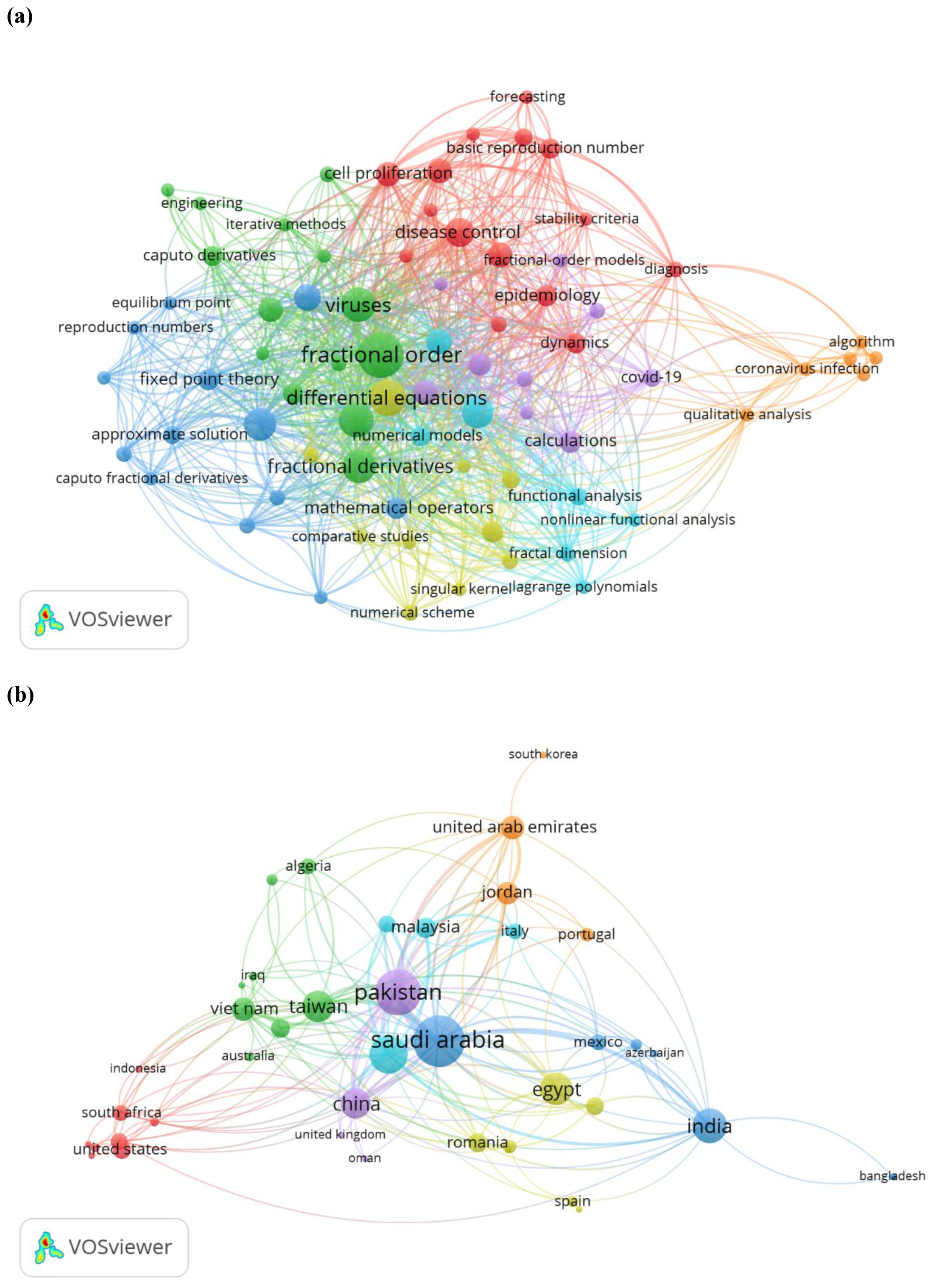
Figure 1. The presentation of the keywords inter-connection on the related literature review studies based on the Scopus database regarding the implementation of fractional-order models for COVID-19. (a) The main keywords of the collected literature review, (b) the main countries focused on this research topic.
Mathematics 11 01036 g001
Figure 2. A diagram for the proposed model of COVID-19.
Mathematics 11 01036 g002
Figure 3. Plot of I ( t ) with κ = 0.996 with the worldwide imported cases of COVID-19 (22 June 2021–24 August 2021). The simulated plot with the above fractional order shows a very good agreement with the real data.
Mathematics 11 01036 g003
Figure 4. Plots of S ( t ) , E ( t ) with different fractional orders. In these plots, the influence of the order of the fractional derivative on the results is clearly visible, the general trend of the plot is maintained, but the resulting numerical values are different.
Mathematics 11 01036 g004
Figure 5. Plots of R ( t ) , D ( t ) with different fractional orders. In these plots, the influence of the order of the fractional derivative on the results is clearly visible, the general trend of the plot is maintained, but the resulting numerical values are different.
Mathematics 11 01036 g005
Figure 6. Plots of I ( t ) with fractional order κ = 0.996 and integer order κ = 1 .
Mathematics 11 01036 g006
Figure 7. Plots of R 0 with respect to parameters ω , γ 1 , γ 2 .
Mathematics 11 01036 g007
Figure 8. Plots of R 0 with respect to parameters λ , τ , β , ϑ .
Mathematics 11 01036 g008
Figure 9. Plots of R 0 with respect to parameters τ , γ 1 , β , γ 2 .
Mathematics 11 01036 g009
Table 1. Comparison between the results of the model for infected group with two types of fractional-order derivatives, Caputo derivative c D κ and Caputo–Fabrizio derivative c f D κ , and reported number of infected people.
t   ( Days ) 102030405060
Real data10,572,13511,946,38513,459,03715,283,45716,719,61318,404,014
c D κ ( κ = 0.996 )10,010,12111,701,24513,041,00415,013,12916,695,92718,925,123
c f D κ ( κ = 0.996 )9,852,91111,024,43912,859,15815,118,25217,251,14920,918,294
Table 2. Comparison between the results of the model for infected group with two types of fractional-order derivatives, Caputo derivative c D κ and Atangana–Baleanu derivative A B C D κ , and reported number of infected people.
t   ( Days ) 102030405060
Real data10,572,13511,946,38513,459,03715,283,45716,719,61318,404,014
c D κ ( κ = 0.996 )10,010,12111,701,24513,041,00415,013,12916,695,92718,925,123
A B C D κ ( κ = 0.996 )9,813,05711,029,15712,918,15014,715,21917,118,40519,581,249
Disclaimer/Publisher’s Note: The statements, opinions and data contained in all publications are solely those of the individual author(s) and contributor(s) and not of MDPI and/or the editor(s). MDPI and/or the editor(s) disclaim responsibility for any injury to people or property resulting from any ideas, methods, instructions or products referred to in the content.