Polynomial Chaos Expansion-Based Enhanced Gaussian Process Regression for Wind Velocity Field Estimation from Aircraft-Derived Data

Abstract

This paper addresses the problem of spatiotemporal wind velocity field estimation for air traffic management applications. Using data obtained from aircraft, the eastward and northward components of the wind velocity field inside a specific air space are calculated as functions of time. Both short-term wind velocity field forecasting and wind velocity field reconstruction are performed. Wind velocity data are indirectly obtained from the states of the aircraft flying in the relevant airspace, which are broadcast by the ADS-B and Mode-S aircraft surveillance systems. The wind velocity field is estimated by combining two data-driven techniques: the polynomial chaos expansion and the Gaussian process regression. The former approximates the global behavior of the wind velocity field, whereas the latter approximates the local behavior. The eastward and northward wind components of the wind velocity field must be estimated, which causes the problem to be a multiple-output problem. This method enables the estimation of the wind velocity field at any spatiotemporal location using wind velocity observations from any spatiotemporal location, eliminating the need for spatial and temporal grids. Moreover, since the method proposed in this article allows for the probability distributions of the estimates to be computed, it causes the computation of the confidence intervals to be possible. Furthermore, since the method presented in this paper allows for data assimilation, it can be used online to continuously update the wind velocity field estimation. The method is tested on different wind scenarios and different training-test data configurations, by means of which the consistency between the results of the wind velocity field forecasting and the wind velocity field reconstruction is checked. Finally, the ERA5 meteorological reanalysis data of the European Centre for Medium-Range Weather Forecasts are used to validate the proposed technique. The results show that the method is able to reliably estimate the wind velocity field from aircraft-derived data.

1. Introduction

1.1. Motivation

Uncertainty is pervasive in the Air Traffic Management (ATM) system, and weather is one of the most significant sources of uncertainty. Four-Dimensional (4D) trajectories will be central elements in the future ATM paradigm; it relies on Trajectory-Based Operations (TBO) because aircraft will be allowed to fly 4D trajectories based on the preferences of the airlines, with the obligation to precisely follow them for traffic synchronization. This means that aircraft trajectories must be predicted with great precision based on reliable meteorological forecasts. Therefore, precise wind information is required to increase trajectory predictability, i.e., the correspondence between planned and actual trajectories [1,2].

Currently, most wind predictions used in aircraft trajectory planning come from Numerical Weather Prediction (NWP) models. NWP meteorological forecasts have a low update rate, typically once every 6 h, and have a coarse spatial resolution. Moreover, observations are mainly gathered from radiosondes, which are launched at specific times, no more than four times per day. All these factors cause using NWP to be inadequate for TBO [3,4]. Therefore, using aircraft-derived data could improve the spatial and temporal resolution of wind forecasts [5].

This paper studies the problem of the spatiotemporal estimation of the wind velocity field within a given air space, in which the eastward and northward components of the wind velocity field are estimated as functions of time using aircraft-derived data. Both short-term wind velocity field forecasting and wind velocity field reconstruction are carried out within a specific air space, in this case, the Terminal Maneuvering Area of the Adolfo Suarez Madrid-Barajas (LEMD) airport, which is located at an altitude of 610 m above sea level. More precisely, the considered airspace is a cuboidal region with a base size of $500\times 500$ km centered at the LEMD airport, with heights ranging from 0.61 km to 14 km. In particular, Mode-S and ADS-B surveillance systems [6,7] will be used in this article to derive the wind velocity, which is indirectly obtained using the relation among the following vectors: the ground speed, the air speed, and the wind velocity itself. A detailed description of the ADS-B and Mode-S technologies can be found in [7].

Several atmospheric data assimilation techniques, which are intended to combine different information sources to estimate the state of the atmosphere, were developed [8]. However, most methods for assimilating these non-conventional aircraft-derived meteorological data are designed to assimilate them into NWP models [9,10,11].

In this article, a different approach to the problem of estimating the state of the atmosphere using aircraft-derived meteorological data is followed. Specifically, the problem of wind velocity field estimation using aircraft-derived wind observations is solved based on a combination of the Polynomial Chaos Expansion (PCE) and the Gaussian Process Regression (GPR) methods, which will be referred to as PCE-GPR. The wind is modeled as a random field with the spatiotemporal position as the input and the wind velocity as the output. The combination of these two techniques is suitable for representing random fields since the PCE models the mean function of the random field and approximates the global behavior of the wind velocity field, whereas the GPR represents the auto-covariance function and approximates the local behavior of such a wind velocity field.

1.2. State of the Art

In [12], a Kalman Filter (KF) was used to estimate the wind speed profile along descent paths using aircraft-derived data. The KF was adapted to account for the uncertainty due to the distance at which observations are collected. This uncertainty was added to the measurement covariance matrix of the KF as a function of the horizontal distance between the observation and estimation locations.

In [13], a novel algorithm for inferring the wind velocity vector from ADS-B data, capable of working in both small and large turning angle situations, is studied. A circle fitting problem is considered, and a sequential least squares optimization algorithm is used.

In [14], the Kriging technique was employed to estimate the wind velocity and temperature fields in the airspace surrounding an airport using aircraft-derived data. Moreover, the same technique was used to predict wind velocity and temperature profiles along descending paths.

In [15], a novel technique that combines particle filtering and Lagrangian transportation was used to partially reconstruct the wind velocity and temperature fields in those regions of the airspace surrounding an airport where a sufficient amount of aircraft-derived data are available. In [16], the technique was further studied, where meteo-particle parameters were optimized and an extrapolation method, based on Delaunay triangulation, to construct a complete wind velocity field was presented.

In [2], the B-splines method was employed to estimate the wind speed profile along descent paths using aircraft-derived data to update the optimal descent trajectory in real-time.

In [17], two approaches to improve the wind velocity data to support TBO are explored: by providing interpolated inter-forecast wind velocity and temperature data and by using aircraft-derived atmospheric observations, such as wind velocity and temperature, to update the forecasted conditions.

In [18], a comparison between several techniques based on the KF and the GPR for wind speed profile estimation from aircraft-derived data in the vertical direction of a given geographical location was conducted, showing that the technique based on the GPR outperforms the methods based on the KF.

In [19], the techniques based on the KF and the GPR for wind speed profile estimation from aircraft-derived data presented in [18] were generalized to wind velocity profile estimation in the vertical direction of a given geographical location, showing that the technique based on the GPR outperforms the methods based on the KF in this case as well.

Finally, in [20], the GPR technique presented in [19] for wind velocity profile estimation in the vertical direction of a given geographical location was extended to the reconstruction and the short-term prediction of the wind velocity field within a given air space. The results showed that the reconstruction has a performance comparable to that of the method proposed in [15] with the advantage of providing an estimate of the entire wind velocity field within a given air space.

In this paper, the PCE is used to enhance the GPR technique. In [21], Wiener first introduced the term PCE for representing the Gaussian distributions using Hermite polynomials.

In [22], the Wiener PCE was extended to other canonical distributions. In [23], the PCE was further extended to arbitrary distributions, which can be specified either analytically, numerically as histograms, or as raw data sets with the introduction of the arbitrary Polynomial Chaos Expansion (aPCE). The aPCE only requires the existence of a finite number of statistical moments and does not rely on the complete knowledge or even on the existence of a probability density function. The aPCE is especially suitable for data-driven applications where no other information is known about the probability distribution of the data, as it eliminates the need to assign parametric probability distributions not sufficiently supported by the available data.

The main contribution of this paper is an innovative method, the PCE-GPR technique, for the reconstruction and short-term prediction of the wind velocity field. The method is iterative and fast, ensuring real-time assimilation of aircraft-derived data is possible. Additionally, the PCE-GPR approach, which previously only allowed for the estimation of scalar output variables, is extended in this study to estimate two output variables: the wind velocity components.

In this paper, the GPR technique employed in [20] is combined with PCE to solve the same problem, generalizing and improving the previous methodology. The PCE-GPR technique was recently introduced in [24] for uncertainty quantification and in [25] for rare event estimation. In both articles, it is referred to as Polynomial Chaos Kriging (PCK). To the best of the authors’ knowledge, the PCE-GPR method has not yet been used for wind velocity field reconstruction and wind velocity field short-term forecasting using aircraft-derived data.

Notice that the terms Kriging and GPR are used interchangeably in the literature. Indeed, GPR and Kriging are essentially the same method, with differences in notation, conceptualization, and in the computation of the confidence intervals of the estimations [26].

The capability of the PCE-GPR method to reconstruct the wind velocity field and to provide short-term predictions within a certain air space was tested using historical aircraft-derived data. Wind velocity observations from two different days characterized by different wind behaviors were chosen. In particular, on the first day, the wind was weaker with a higher degree of directional dispersion, whereas, on the second day, it was stronger with a lower degree of directional dispersion. The data sets were split into training and test sets in two different ways, namely by randomly selecting sets of individual observations and by randomly selecting sets of flights. Moreover, the wind velocity field estimates obtained through the PCE-GPR method were validated using the meteorological reanalysis data retrieved from the ERA5 repository of the European Centre for Medium-Range Weather Forecasts (ECMWF). The results of the validation show that the estimates are consistent with the reanalysis data, demonstrating the capability of the method presented in this article to estimate the wind velocity even in those regions of the air space in which a reduced number of observations are available.

The paper is structured as follows. The procedure for obtaining the aircraft-derived data and the results of the exploratory analysis of the obtained data sets are described in Section 2.1. The GPR technique is introduced in Section 2.2, and the mathematical development of the PCE method is described in Section 2.3. The combination of both methods is explained in Section 2.4, and the extension of the PCE-GPR method to multi-output processes is presented in Section 2.5. The results of the numerical experiments are described in Section 3 and discussed in Section 4. Finally, Section 5 contains the conclusions.

2. Methods

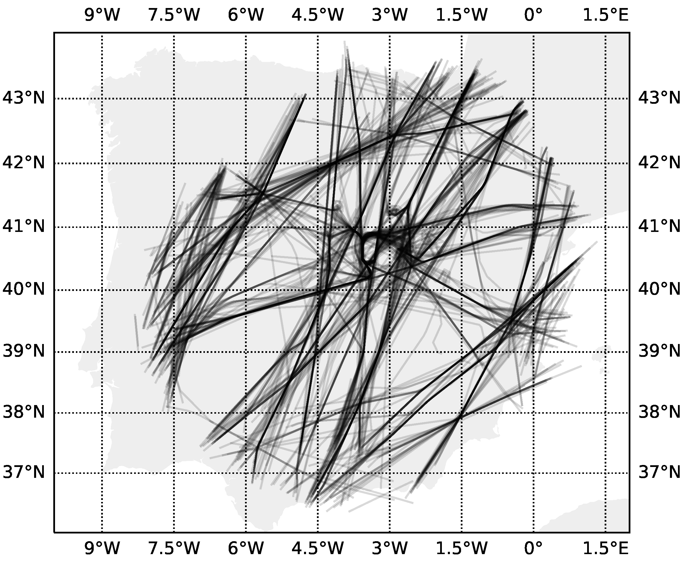
2.1. Data Derivation and Exploratory Analysis

This section presents the procedure through which the wind velocity information is derived from the ADS-B and Mode S data. In addition, the main results of the exploratory analysis of these aircraft-derived data are also summarized.

2.1.1. Data Source

The data employed in this work were supplied by the Spanish Air Navigation Service Provider (ENAIRE). Specifically, the data were extracted from the All-Purpose Structured EUROCONTROL Surveillance Information Exchange (ASTERIX) database, which contains a great amount of flight information, as described in the technical reports of EUROCONTROL [27], from which the ADS-B [28] and Mode-S [29] data were obtained. More precisely, two data sets were extracted from this database. The observations of the first data set, which contains data with lower wind speeds and higher dispersion in the wind direction, correspond to 23 February 2020. It will be referred to as the Day 1 data set. The observations of the second data set, which contains data with higher wind speeds and lower dispersion in the wind direction, correspond to 21 December 2019. It will be referred to as the Day 2 data set. The observations in both data sets were obtained from 08:00 to 14:00 UTC, which corresponds to the time period with the maximum level of traffic at the LEMD airport.

2.1.2. ADS-B and Mode S Systems

The ADS-B system automatically transmits the position and ground speed of the aircraft approximately every 0.5 s. Mode S is a selective interrogation system used to transmit additional flight information. Aircraft are interrogated by surveillance radars and reply through a transponder by means of the so-called Mode S Enhanced Surveillance communication protocol. In fact, the Mode S extended squitter transponder is the most common implementation of ADS-B. In particular, as described in [29], binary data store registers 50 and 60 contain the information necessary for deriving the wind velocity, as it will be explained in Section 2.1.3. For further details on surveillance technologies, the reader is referred to [7].

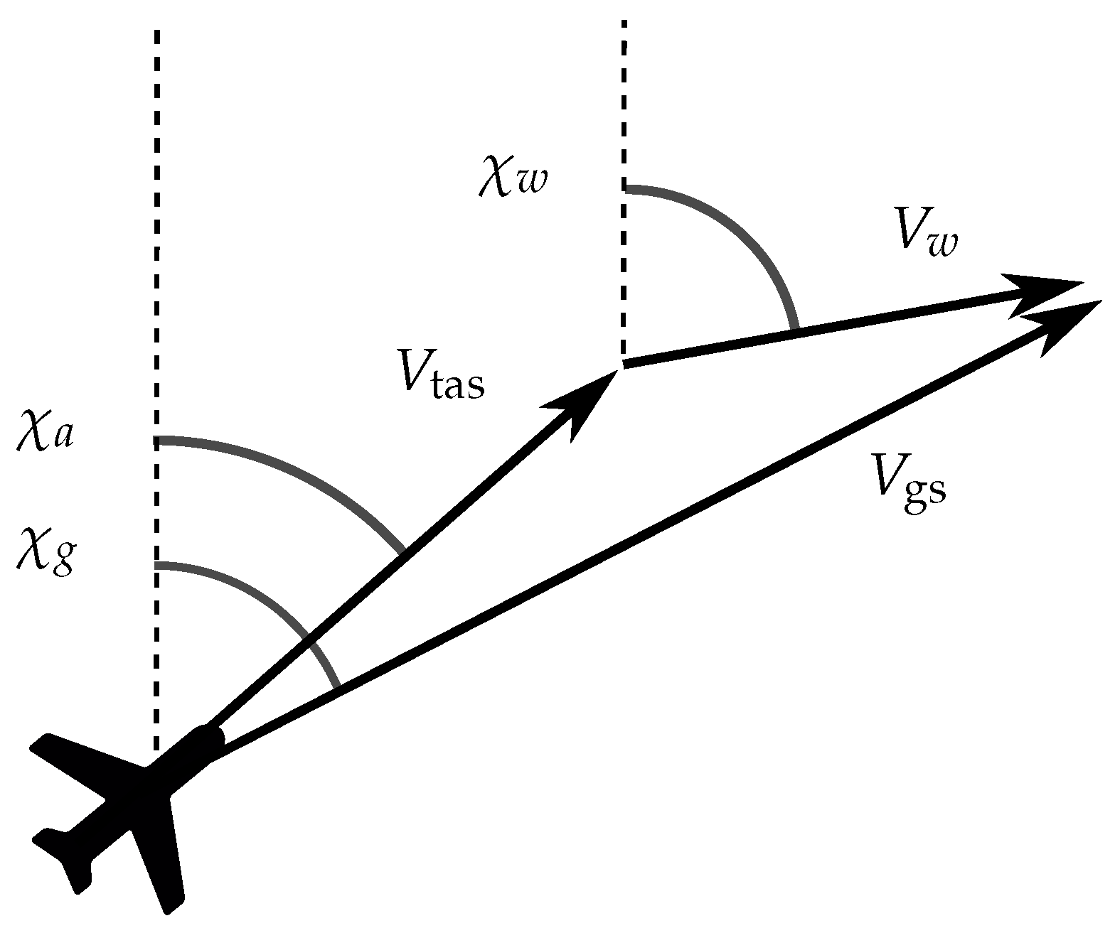
2.1.3. Wind Velocity Derivation from ADS-B and Mode S Data

The vector that represents the wind velocity can be obtained as the difference between the vectors that represent the ground speed and the actual airspeed using the true airspeed, the ground speed, and the heading and track angles. The relationship between the ground speed, true airspeed, and wind velocity vectors, denoted as $V_{gs}$, $V_{tas}$, and $V_w$, respectively, is shown in Figure 1, where ${\chi }_g$, ${\chi }_a$, and ${\chi }_w$ represent the track angle, the heading angle, and the wind direction angle, respectively. Thus, the wind velocity data sets employed in this work were built from the wind velocity observations derived from different aircraft states, which were obtained through the ADS-B and Mode-S surveillance technologies.

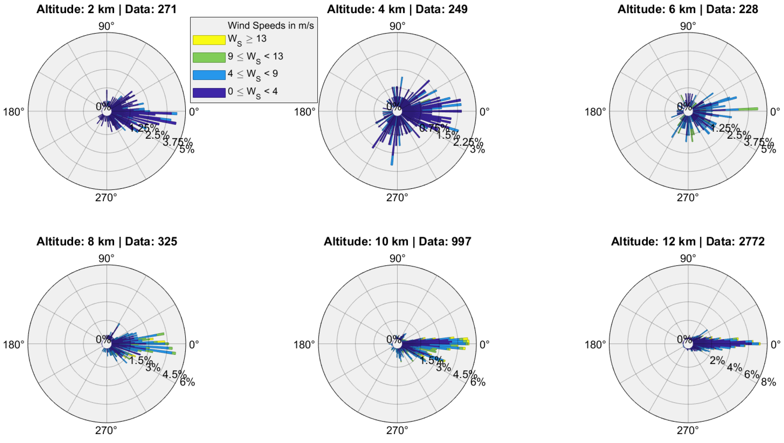
2.1.4. Exploratory Data Analysis

Table 1. Main statistics of the wind velocity.

	Wind Speed (m/s)		Wind Direction (Deg)
	Day 1	Day 2	Day 1	Day 2
Min.	0	0.013	0.01	163.79
Max.	56.04	100.75	359.99	351.55
Mean	17.80	60.56	307.16	166.66
Dispersion	11.30	16.67	19.40 (%)	2.11 (%)

shows the main statistics of the wind velocity of the Day 1 and Day 2 data sets. Circular statistics were used to compute the mean and dispersion of angles [30]. It can be seen that the average wind speed in the Day 2 data set is around 3 times larger than in the Day 1 data set, whereas the dispersion of the wind direction is about 10 times lower. The dispersion of the wind direction, in circular statistics, is measured by a percentage. A 100% dispersion means that the direction of the wind velocity observations is uniformly distributed in all directions, whereas a 0% dispersion means that all the wind velocity observations have the same direction.

The spatial configuration of the Day 1 data set is represented in Figure 2, in which the coverage region over the Iberian Peninsula, together with the flight routes, can be observed. Using this kind of data set to estimate wind velocity fields is a challenging task, since they are non-uniformly distributed in the air space.

For a detailed exploratory analysis of these two data sets, the reader is referred to [20].

2.2. Gaussian Process Regression

Gaussian Processes (GP) are stochastic processes that allow for a wide variety of properties to be modeled, including linearity, continuity, smoothness, differentiability, symmetry, and periodicity. GP can be completely determined by their mean and covariance functions. The deterministic trends of the GP are represented by the mean functions, whereas their stochastic properties are described by the covariance functions, which are usually referred to as kernel functions.

GPR may be thought of as a general regression model, which can be employed in many research areas, such as machine learning [31] or functional data analysis [32]. Given some predictor variables $\mathbf{x}=(x_1,x_2,\dots ,x_d)$, a GPR model provides a prediction $\mathcal{M}\left(x\right)$ of the value of a scalar output variable y, assuming the mapping $y=\mathcal{M}\left(x\right)$ to be a realization of a Gaussian random process, and generalizing the linear regression model

$$y={\mathbf{x}}^T\mathit{\beta }+\epsilon ,$$

(1)

in which $\epsilon \sim N(0,{\sigma }^2)$, $\mathit{\beta }=({\beta }_1,{\beta }_2,\dots ,{\beta }_d)$ represent the parameters of the regression model, and ${\sigma }^2$ denotes the error variance.

GPR introduces a new term $f\left(\mathbf{x}\right)$ in the linear model (1), which is assumed to be a Gaussian process, i.e., it is assumed that, jointly, the random variables $\left\{f\left({\mathbf{x}}_1\right),f\left({\mathbf{x}}_2\right),f\left({\mathbf{x}}_3\right),\dots ,f\left({\mathbf{x}}_n\right)\right\}$ have zero-mean Gaussian distribution with covariance function $K(\mathbf{x},{\mathbf{x}}^{\prime })$, for any collection of observations $\left\{{\mathbf{x}}_1,{\mathbf{x}}_2,\dots ,{\mathbf{x}}_n\right\}$. Additionally, the linear term in (1) is replaced by a basis function $h(·)$, which projects the predictor variable $\mathbf{x}$ into a p-dimensional feature space. Thus, the GPR model can be formulated as:

$$y=\mathcal{M}\left(\mathbf{x}\right)=h{\left(\mathbf{x}\right)}_{1\times p}^T{\mathit{\beta }}_{p\times 1}+f\left(\mathbf{x}\right)+\epsilon .$$

(2)

Given a set of observations $(\mathcal{X},\mathcal{Y})=\left\{({\mathbf{x}}^j,y^j),j=1,2,\dots ,n\right\}$ that relate the input variables $\mathbf{x}$ with the output variable y through the GPR model (2), it can be shown that $\widehat{y}$, the predicted output variable at point $\widehat{\mathbf{x}}$, is also Gaussian distributed [31]. As a consequence, GPR is able to provide both an estimation of the output variable and its associated probability distribution.

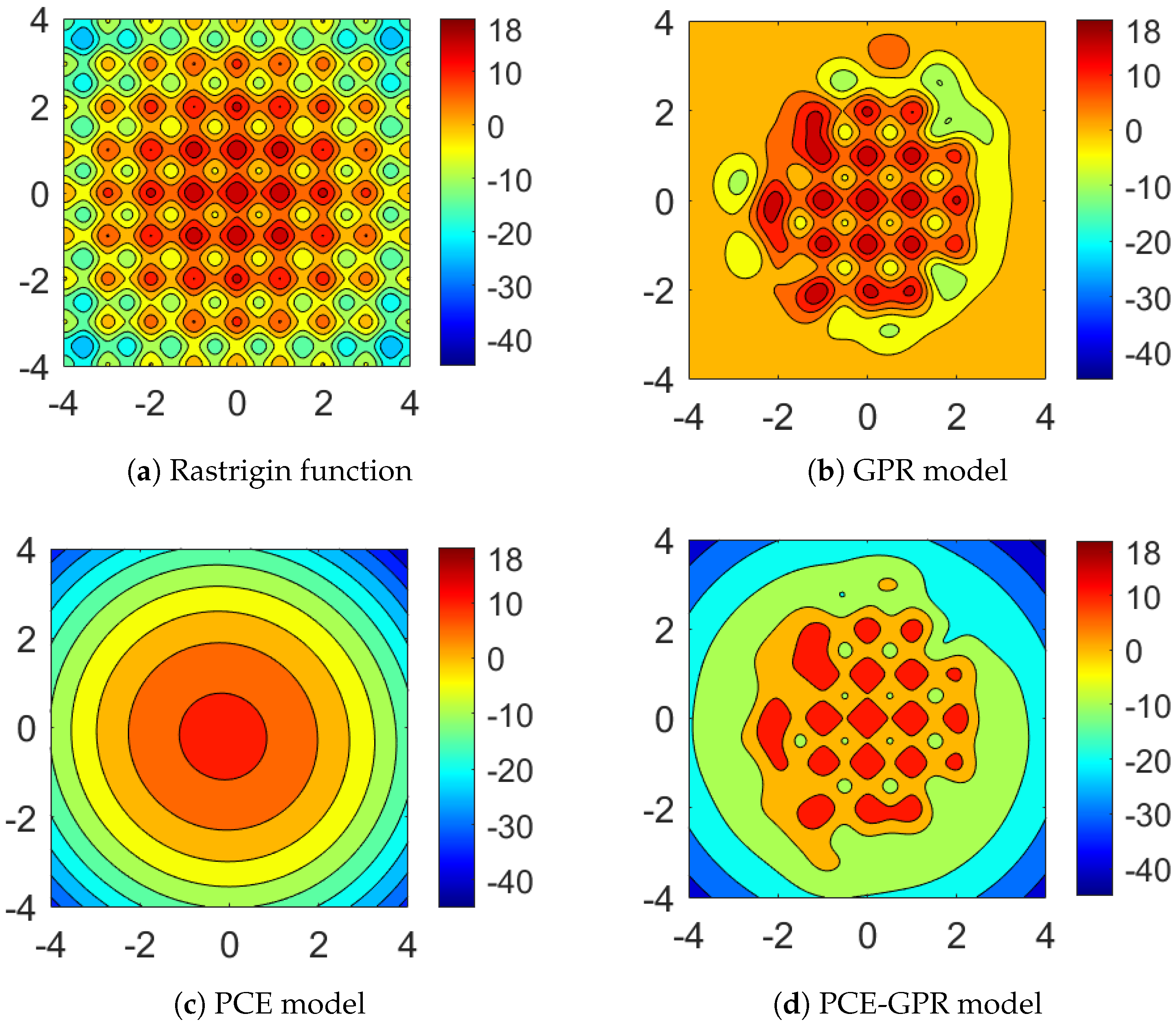
2.3. Polynomial Chaos Expansion

Following [33], this section presents the PCE method, which allows for the computation of an analytical model that maps an input random vector onto an output random variable under certain hypotheses.

Let $(\mathsf{\Omega },\mathcal{F},\mathcal{P})$ be a probability space, with $\mathsf{\Omega }$ the space of events, $\mathcal{F}$ a $\sigma$-algebra, and $\mathcal{P}$ a probability measure. Assume that there exists an unknown deterministic mapping $\mathcal{M}$ from a d-dimensional input parameter space to a one-dimensional output space, namely $\mathcal{M}:{\mathbb{R}}^d\to \mathbb{R}$, such that $y=\mathcal{M}\left(\mathbf{x}\right)$, with $\mathbf{x}=(x_1,x_2,\dots ,x_d)$.

If the input vector x is assumed to be affected by uncertainties, it can be represented by a random vector $\mathbf{X}=(X_1,X_2,\dots ,X_d)$ with a joint Probability Density Function (PDF) $f_{\mathbf{X}}=(f_{X_1},f_{X_2},\dots ,f_{X_d})$, and then $Y=\mathcal{M}\left(\mathbf{X}\right)$ is an output random variable, which is obtained by propagating the input vector uncertainties through the mapping $\mathcal{M}$.

PCE is a spectral decomposition method that provides a computationally efficient way to calculate an analytical representation that maps the input random vector $\mathbf{X}$ onto the output random variable Y, under two hypotheses. The output random variable Y is assumed to be a second-order variable, namely:

$$E\left[Y^2\right]={\int }_{{\mathbb{R}}^d}{\mathcal{M}}^2\left(\mathbf{x}\right)f_{\mathbf{X}}\left(\mathbf{x}\right)d\mathbf{x}<+\infty .$$

Additionally, each component $X_i,i=1,2,\dots ,d$, of the input random vector $\mathbf{X}$ is assumed to have finite moments of all orders.

Provided that these two assumptions are fulfilled, the output random variable Y can be represented by the following PCE

$$Y\left(\mathbf{X}\right)=\mathcal{M}\left(\mathbf{X}\right)=\sum _{\mathbf{\alpha }\in {\mathbb{N}}^d}{c}_{\mathbf{\alpha }}{\mathsf{\Psi }}_{\mathbf{\alpha }}\left(\mathbf{X}\right),$$

(3)

where $\{c_{\mathbf{\alpha }},\mathbf{\alpha }\in {\mathbb{N}}^d\}$ are the coefficients of the expansion and $\{{\mathsf{\Psi }}_{\mathbf{\alpha }}(·),\mathbf{\alpha }\in {\mathbb{N}}^d\}$ is a basis of polynomials orthonormal with respect to the probability measure $\mathcal{P}$ represented by the joint PDF $f_{\mathbf{X}}$, namely

$${\int }_{{\mathbb{R}}^d}{\mathsf{\Psi }}_{\mathbf{\alpha }}\left(\mathbf{x}\right){\mathsf{\Psi }}_{\mathbf{\beta }}\left(\mathbf{x}\right)f_{\mathbf{X}}\left(\mathbf{x}\right)d\mathbf{x}={\delta }_{\mathbf{\alpha }\mathbf{\beta }},$$

(4)

with ${\delta }_{\mathbf{\alpha }\mathbf{\beta }}$ denoting the Kronecker delta and $\mathbf{\alpha },\mathbf{\beta }\in {\mathbb{N}}^d$ representing multi-indexes.

Assuming that the input random vector $\mathbf{X}$ has statistically independent components, each multivariate polynomial ${\mathsf{\Psi }}_{\mathbf{\alpha }}$ of the PCE basis $\{{\mathsf{\Psi }}_{\mathbf{\alpha }}(·),\mathbf{\alpha }\in {\mathbb{N}}^d\}$ can be computed as the tensor product of d univariate orthogonal polynomials as follows

$${\mathsf{\Psi }}_{\mathbf{\alpha }}\left(\mathbf{x}\right)=\prod _{i=1}^d{\psi }_{{\mathbf{\alpha }}_i}^{\left(i\right)}\left(x_i\right),$$

(5)

where each univariate polynomial ${\psi }_{{\mathbf{\alpha }}_i}^{\left(i\right)}(·)$, $i=1,2,\dots ,d$, is the component of degree ${\alpha }_i$ of a basis of univariate polynomials orthonormal with respect to the marginal PDF $f_{X_i}$ of $\mathbf{X}$, namely the PDF of the random variable $X_i$. The component ${\alpha }_i$ of the multi-index $\mathbf{\alpha }=({\alpha }_1,{\alpha }_2\dots ,{\alpha }_d)\in {\mathbb{N}}^d$ designates the degree of the multivariate polynomial ${\mathsf{\Psi }}_{\mathbf{\alpha }}$ in the i-variable, for $i=1,2,...,d$. The total degree of ${\mathsf{\Psi }}_{\mathbf{\alpha }}$ is calculated as $\left|\mathbf{\alpha }\right|={\sum }_{i=1}^d{\alpha }_i$.

In practice, the infinite terms of the PCE (3) must be truncated to a finite sum. There are different ways to choose a truncation scheme, in which a set of multi-indexes is selected. The most commonly used truncation scheme consists of setting an upper bound p on the total degree $\left|\mathbf{\alpha }\right|$ of the multivariate polynomials ${\mathsf{\Psi }}_{\mathbf{\alpha }}$, namely the set of multi-indexes:

$${\mathcal{A}}^{d,p}=\{\mathbf{\alpha }\in {\mathbb{N}}^d:\left|\mathbf{\alpha }\right|\le p\}.$$

(6)

Thus, the truncated PCE that approximates the infinite series (3) can be formulated as

$$Y_{PC}\left(\mathbf{X}\right)={\mathcal{M}}_{PC}\left(\mathbf{X}\right)=\sum _{k=1}^{|{\mathcal{A}}^{d,p}|}{c}_k{\mathsf{\Psi }}_k\left(\mathbf{X}\right),$$

(7)

where

$$|{\mathcal{A}}^{d,p}|=\frac{(d+p)!}{d!p!}.$$

There are different ways to construct the basis of orthonormal polynomials $\{{\mathsf{\Psi }}_{\mathbf{\alpha }}(·),\mathbf{\alpha }\in {\mathbb{N}}^d\}$. In general, the computation of each ${\mathsf{\Psi }}_{\mathbf{\alpha }}$ requires the availability of the marginal distributions of $X_i,i=1,2,\dots ,d$, which are employed in the tensor product (5). However, a wide variety of univariate distributions is associated with a specific family of orthonormal polynomials [22]. In this case, it is straightforward to compute the basis of orthonormal polynomials. For instance, the Hermite polynomials are associated with the Gaussian distribution.

When the distributions of the input random variables $X_i,i=1,2,\dots ,d$, have no family of orthonormal polynomials associated, a common approach consists of directly constructing the basis of orthonormal polynomials using Stiltjes or Gram–Schmidt orthogonalization [34].

As mentioned in the Introduction, a more general approach is the aPCE [23], which consists of constructing the basis of orthonormal polynomials from the statistical moments of the input random variables $X_i,i=1,2,\dots ,d$. Thus, this approach does not require the availability or even the existence of a functional representation of the marginal PDFs $f_{X_i},i=1,2,\dots ,d$. However, in the aPCE approach a large number of input samples is necessary for an accurate estimation of higher order moments [35].

In this paper, the Kernel Density Estimation (KDE) [36] was employed to estimate the marginal PDFs $f_{X_i},i=1,2,\dots ,d$, and then the Stiltjes orthogonalization was used to build the corresponding basis of the orthonormal polynomials. More specifically, given a set ${\mathcal{X}}_i=\left\{x_i^1,x_i^2,\dots ,x_i^n\right\}$ of n observations of the input random variable $X_i$, the kernel density estimate of the marginal PDF $f_{X_i}$ was calculated as

$${\widehat{f}}_{X_i}\left(x\right)=\frac{1}{n\eta }\sum _{j=1}^{n}K\left(\frac{x-x_i^j}{\eta }\right),$$

(8)

where $K(·)$ represents the kernel function and $\eta$ denotes an appropriate kernel bandwidth. In particular, a Gaussian kernel was used, and the corresponding kernel bandwidth was learned from the set of observations ${\mathcal{X}}_i$ by means of the Silverman’s rule [37].

Once the truncation scheme (6) was selected, the coefficients $c_k,k=1,2,\dots ,\left|{\mathcal{A}}^{d,p}\right|$, of the truncated expansion (7) can be calculated using different approaches, such as Galerkin projection, collocation, numerical integration, or regression [22].

In this paper, given a set of observations of the input random vector and the corresponding output random variable, namely $(\mathcal{X},\mathcal{Y})=\left\{({\mathbf{x}}^j,y^j),j=1,2,\dots ,n\right\}$ the expansion coefficients have been estimated using regression. More specifically, the vector of expansion coefficients $\mathbf{c}=(c_1,c_2,\cdots ,c_{|{\mathcal{A}}^{d,p}|})$ was estimated by solving the least squares minimization problem:

$$\widehat{\mathbf{c}}=\underset{\mathbf{c}\in {\mathbb{R}}^{|{\mathcal{A}}^{d,p}|}}{arg\; min}\sum _{j=1}^n{\left(y^j-Y_{PC}\left({\mathbf{x}}^j\right)\right)}^2=\underset{\mathbf{c}\in {\mathbb{R}}^{|{\mathcal{A}}^{d,p}|}}{arg\; min}\sum _{j=1}^n{\left(y^j-\sum _{k=1}^{|{\mathcal{A}}^{d,p}|}{c}_k{\mathsf{\Psi }}_k\left({\mathbf{x}}^j\right)\right)}^2.$$

(9)

In particular, the vector of expansion coefficients $\widehat{\mathbf{c}}$ estimated in (9) was calculated as

$$\widehat{\mathbf{c}}={\left({\mathbf{A}}^T\mathbf{A}\right)}^{-1}{\mathbf{A}}^T\left(\begin{array}{c}{y}^1\\ y^2\\ ⋮\\ y^n\end{array}\right),$$

where $a_{jk}={\mathsf{\Psi }}_k\left({\mathbf{x}}^j\right),j=1,2,\dots ,n,k=1,2,\dots ,\left|{\mathcal{A}}^{d,p}\right|$, are the entries of matrix $\mathbf{A}$.

2.4. Polynomial Chaos Expansion-Based Enhanced Gaussian Process Regression

As explained in Section 2.2, the GPR model (2) interpolates local variations of the output variable y as a function of experimental observations of the predictor variables $\mathbf{x}$, whereas the PCE model (3) approximates the global behavior of the mapping $y=\mathcal{M}\left(\mathbf{x}\right)$ by means of a set of orthonormal polynomials, as described in Section 2.3. Therefore, as pointed out in [24], the aim of combining PCE and GPR is to capture at the same time both the global behavior and the local variability of the mapping that relates the output variable y to the predictor variables $\mathbf{x}$. To this end, the trend of the GPR model (2), represented by the term $h{\left(\mathbf{x}\right)}_{1\times p}^T{\mathbf{\beta }}_{p\times 1}$, is replaced by the truncated PCE (7), so that the PCE-GPR model can be formulated as follows:

$$y=\mathcal{M}\left(\mathbf{x}\right)=\sum _{k=1}^{|{\mathcal{A}}^{d,p}|}{c}_k{\mathsf{\Psi }}_k\left(\mathbf{x}\right)+f\left(\mathbf{x}\right)+\epsilon .$$

(10)

The ability of capturing local and global properties through the PCE-GPR model (10) is analyzed in [24] through several benchmark analytical functions, such as the Rastrigin function [38], which is a two-dimensional function that combines a quadratic term and a high-frequency trigonometric term. The contour plot of the Rastrigin function is illustrated in Figure 3a–d to show the approximations of the Rastrigin function by the GPR, PCE, and PCE-GPR models, which were generated using 128 sample points from a standard normal bivariate distribution, respectively.

It can be seen in Figure 3b that the GPR model properly approximates the local extrema of the Rastrigin function, whereas the global feature of the function is barely learned by this model. Conversely, Figure 3b shows how the PCE model reproduces the global behaviour of the Rastrigin function while missing out on the local extrema. Finally, the capability of the PCE-GPR model to combine both characteristics of the Rastrigin function is illustrated in Figure 3d.

2.5. Adaptation of PCE-GPR to the Wind Velocity Output

As mentioned before, this paper addresses the problem of spatiotemporal wind velocity field estimation. More specifically, the eastward and northward components of the wind velocity, which will be referred to as u and v components, respectively, are inferred at different altitudes as functions of time from aircraft-derived data. Therefore, the single output PCE-GPR model described in Section 2.4 must be extended to this multiple-output setting.

The GPR method cannot be directly generalized to multi-output processes in a unique and effective way. The ability of the GPR model to estimate multiple-outputs, seeking to take advantage of the knowledge about the relation between them, is still a field of active research. Usually, a covariance function describing both the auto-correlation of the output variables as well as the correlation among them is included in the formulation of the model [39]. However, the formulation of a covariance function for multiple correlated output variables is a difficult task. Besides, the estimation efficiency of a GPR model can be significantly reduced if the covariance structure among outputs is mis-specified [40]. Therefore, the common approach in practice is to address these estimation problems by means of independent single-output GPR models.

In this paper, the following approach was followed to adapt the PCE-GPR method to the wind velocity output. First, the wind speed and wind direction were predicted using three outputs, namely $(y_1,y_2,y_3)=(r,cos\gamma ,sin\gamma )$, with r being the wind speed and $\gamma$ the wind velocity direction. Then, the u and v components were retrieved as $(u,v)=(rcos\gamma ,rsin\gamma )$.

The motivation behind this approach is threefold. The estimation of the wind velocity using independent single-output GPR models has already been proven to be effective in [20]. Moreover, since they are two different physical magnitudes, the separation between the wind speed and the wind direction predictions benefits the training process of the PCE-GPR model. Finally, because each of the three output variables $(y_1,y_2,y_3)$ are trained independently, parallel computing can be used.

3. Results

3.1. Model Set Up

In this section, the PCE-GPR model layout is presented, namely the selection of the model parameters, which include the total degree of the truncated PCE expansion, the hyperparameter vector of the kernel function, and the error standard deviation.

The total degree p of the truncated PCE expansion included in (10) was selected between 1 and 10. More specifically, the value of p that provides the least leave-one-out error, ${ϵ}_{LOO}$, was chosen, where

$${ϵ}_{LOO}=\frac{1}{n}\sum _{j=1}^n{\left(\frac{y^j-Y_{PC}\left({\mathbf{x}}^j\right)}{1-{\nu }_j}\right)}^2,$$

with ${\nu }_j,j=1,2,\dots ,n$, being the jth diagonal term of the matrix $\mathbf{A}{\left({\mathbf{A}}^T\mathbf{A}\right)}^{-1}{\mathbf{A}}^T$ [24].

The covariance function in (10) was computed using the squared exponential kernel [31], namely

$$K(\mathbf{x},{\mathbf{x}}^{\prime }|\theta )={\sigma }_{\mathrm{f}}^2{e}^{-R^2},$$

(11)

with

$$R=\sqrt{\sum _{i=1}^d\frac{{(x_i-x_i^{\prime })}^2}{{\sigma }_i^2}},$$

where $\theta =({\sigma }_f,{\sigma }_1,{\sigma }_2,{\sigma }_3,{\sigma }_4)$ is the hyperparameter vector and $d=4$, since the components of the input vector x are the coordinates of the spatiotemporal position of the aircraft. The kernel function (11) produces continuous and smooth GP samples, thus providing a smooth regression capable of uniformly approximating any continuous function on a compact subset contained in the input space [41].

Moreover, the correlation between two spatiotemporal input points decreases as a function of the weighted Euclidean distance. Since, in the wind velocity estimation the input variables have different length scales, each input variable $x_i,i=1,2,3,4$, in the kernel function (11) was scaled by a factor ${\sigma }_i^2$. The hyperparameter ${\sigma }_f$, referred to as the signal standard deviation, allows the auto-covariance to be adapted to the output scale. To achieve a fast and accurate estimation of the hyperparameter vector $\theta$, the subset of the data method [31], together with the block coordinate descent approximation [42], were used during the training phase of the model.

Finally, according to [12], the standard deviation $\sigma$ of the model error $\epsilon$ in (10) was set to 3 m/s, which is the typical wind instrumental error.

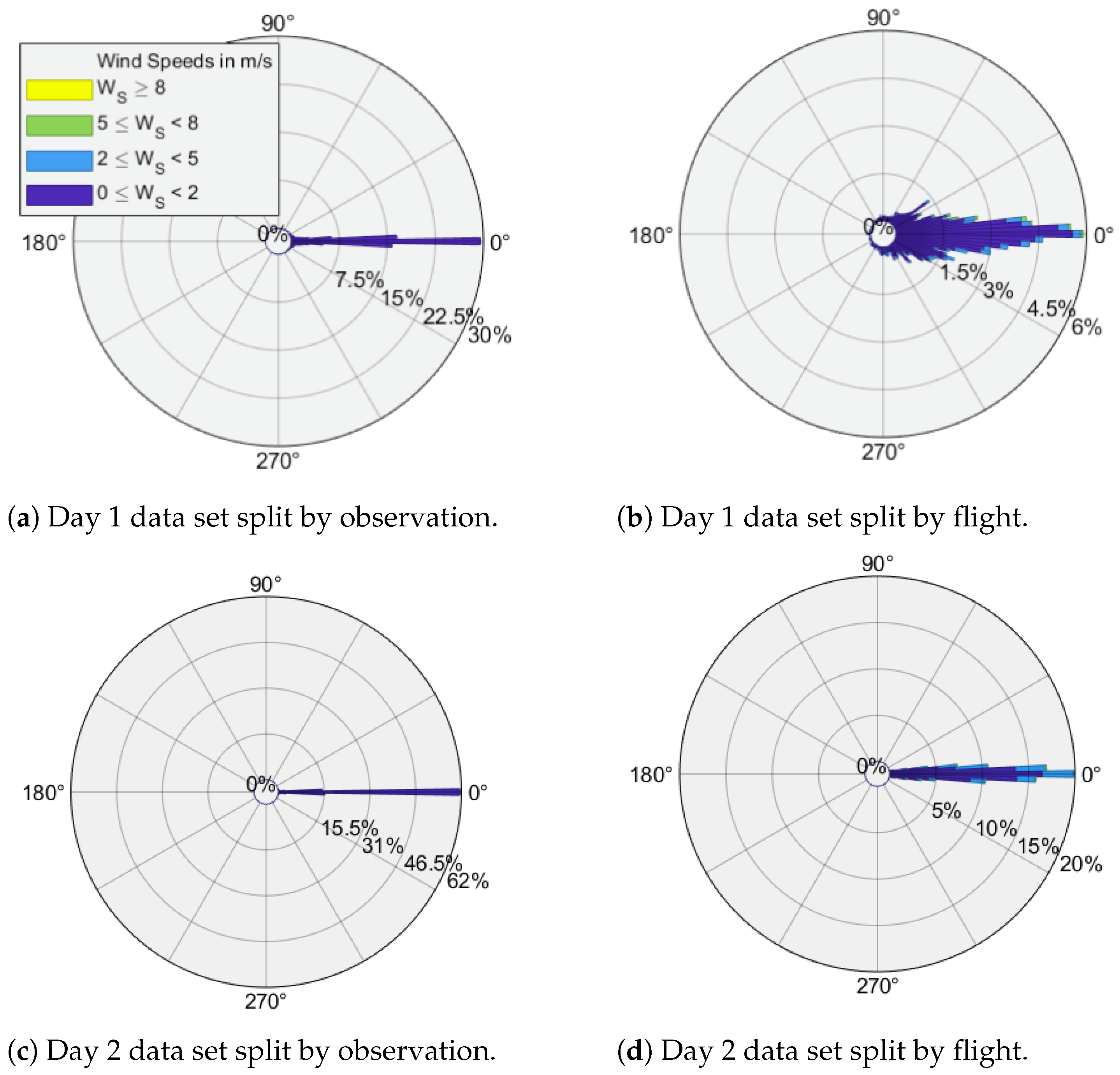
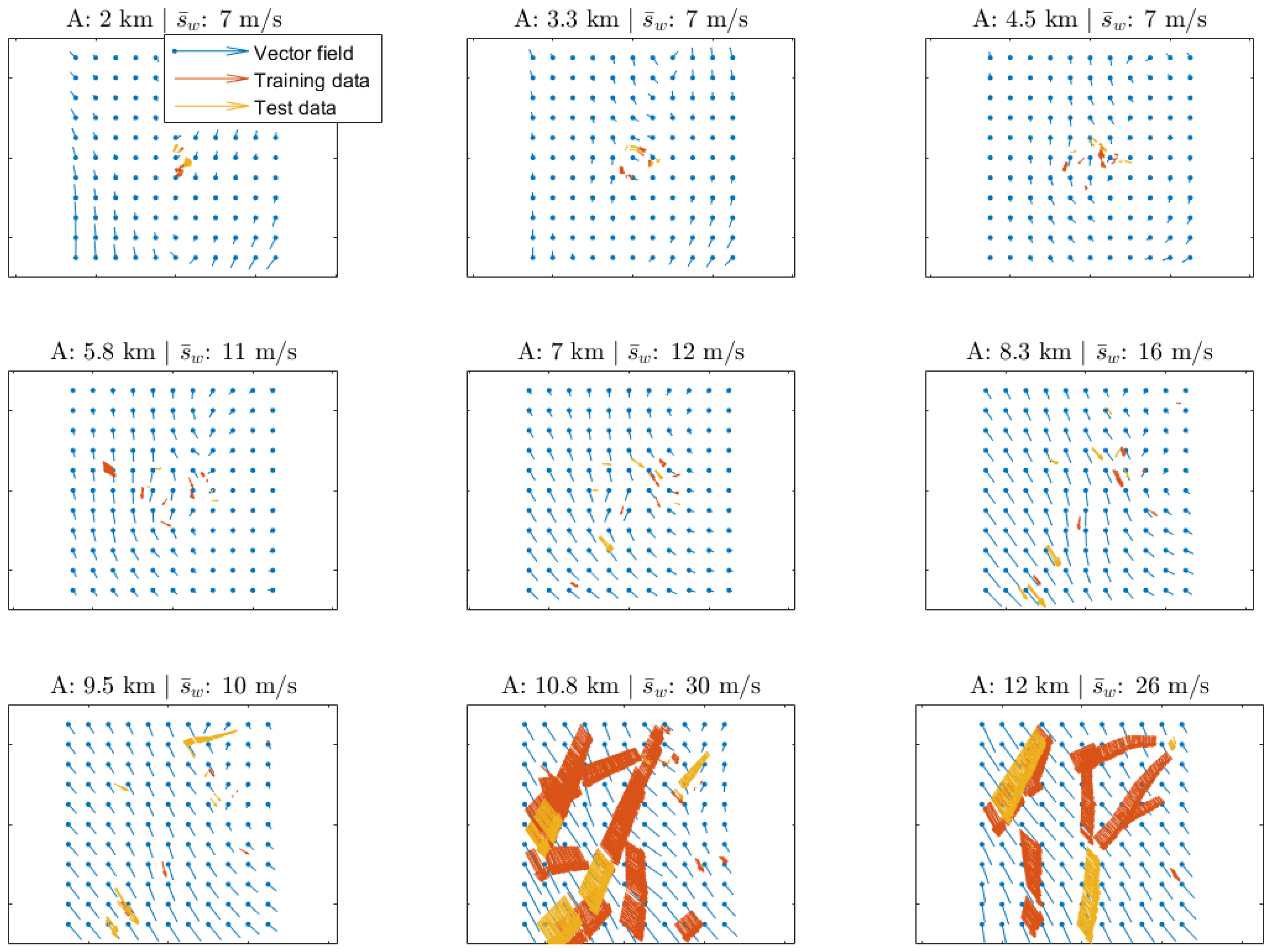
3.2. Wind Velocity Field Reconstruction

The capability of the PCE-GPR method to reconstruct the wind velocity fields within a particular air space using historical aircraft-derived data is studied in this section. More specifically, the wind velocity field was reconstructed around the LEMD airport employing the wind velocity data sets introduced in Section 2.1.1 using data collected over a one-hour period. In particular, a cuboidal region centered at the LEMD airport with base size $500\times 500$ km and altitude ranging between 0.6 km and 14 km was used. Moreover, both aircraft-derived data sets were split into training and test sets using two different approaches:

• By randomly choosing sets of individual observations, which will be referred to as data set randomly split by observation.
• By randomly selecting sets of flights, employing the individual observations gathered from them, which will be referred to as a data set randomly split by flight.

Specifically, in both cases, $20\%$ of the data were kept for testing to assess the accuracy of the wind velocity field reconstruction. Thus, four different PCE-GPR models were trained. The computational time of the training phase for each of these models was less than 5 min.

Three different measurements of the estimation error were computed for each of the four models, namely the Root Mean Square Error (RMSE), the Mean Absolute Error (MAE), and the Median Absolute Deviation (MAD), which are reported in

Table 2. Wind velocity field reconstruction: Estimation errors for the u and v components of the wind velocity.

		Data Set Split by Observation		Data Set Split by Flight
Measure of Error	Component	Day 1	Day 2	Day 1	Day 2
RMSE (m/s)	u	2.26 (18%)	1.50 (21%)	5.84 (1%)	6.06 (−4%)
	v	1.46 (44%)	1.45 (22%)	4.79 (14%)	4.84 (1%)
MAE (m/s)	u	1.17 (22%)	0.99 (22%)	4.46 (−1%)	4.37 (−2%)
	v	0.83 (43%)	1.05 (19%)	3.45 (13%)	3.59 (3%)
MAD (m/s)	u	0.53 (23%)	0.64 (22%)	3.60 (−6%)	3.03 (−2%)
	v	0.49 (31%)	0.80 (15%)	2.44 (9%)	2.70 (5%)

.

It can be seen that the values of the estimation errors of the wind velocity components for both the Day 1 and Day 2 data sets are similar. Conversely, the values of the estimation errors significantly differ depending on the data splitting procedure chosen. This is due to the fact that the spatiotemporal distance between the training and test observations is higher when the data sets are randomly split by flight, which causes the estimation to be more challenging.

Table 2 also reports, between parentheses, the relative improvement obtained in comparison with the values of the estimation errors reported in [20], in which the wind velocity field reconstruction was carried out using the GPR method without the enhancement provided by the PCE. It can be seen that the PCE-GPR method considerably outperforms the GPR method when the data sets are randomly split by observation, whereas the incorporation of the PCE into the GPR model does not statistically improve the estimation errors already achieved when the data sets are randomly split by flight.

Figure 4 shows the rose diagrams of the wind velocity estimation errors for each of the four models, which can be thought of as circular histograms. The values in the inner circumferences represent percentages of the total data set, whereas the quantities in the outer circumference denote angles representing the wind velocity direction errors that are expressed in degrees. Moreover, a color scale is used to indicate the wind speed. It can be seen that the estimation errors of the wind velocity direction are symmetrically distributed around 0 degrees, showing a low dispersion. Moreover, the dispersion is particularly low when the data sets are randomly split by observation. Likewise, the estimation errors of the wind speed adopt low values, ranging between 0 and 5 m/s.

The wind velocity fields reconstructed using the PCE-GPR method from the Day 1 data set, at a given instant in time and for different altitudes ranging from 2 to 12 km, are shown in Figure 5, together with the value of the associated mean wind speed ${\overline{s}}_w$. A selection of members of the corresponding training and test data sets are also depicted. It can be observed that the reconstructed wind velocity fields properly fit the data and behave smoothly.

In addition, to complement Figure 5, the rose diagrams that represent the wind velocity estimation errors segmented by height are shown in Figure 6. It can be seen that, at altitudes below 10 km, the wind speed is low, ranging from 0 km/h to 36 km/h, and the wind direction variability is high. This effect can be observed in the first three rose diagrams.

The reconstruction of the wind speed dynamics from 14:10 to 15:00 UTC at cruise altitude (10.3 km) for the Day 2 data set is illustrated in Figure 7 by means of an isotach map. It can be seen how the contour bars gradually change over the considered space and time period.

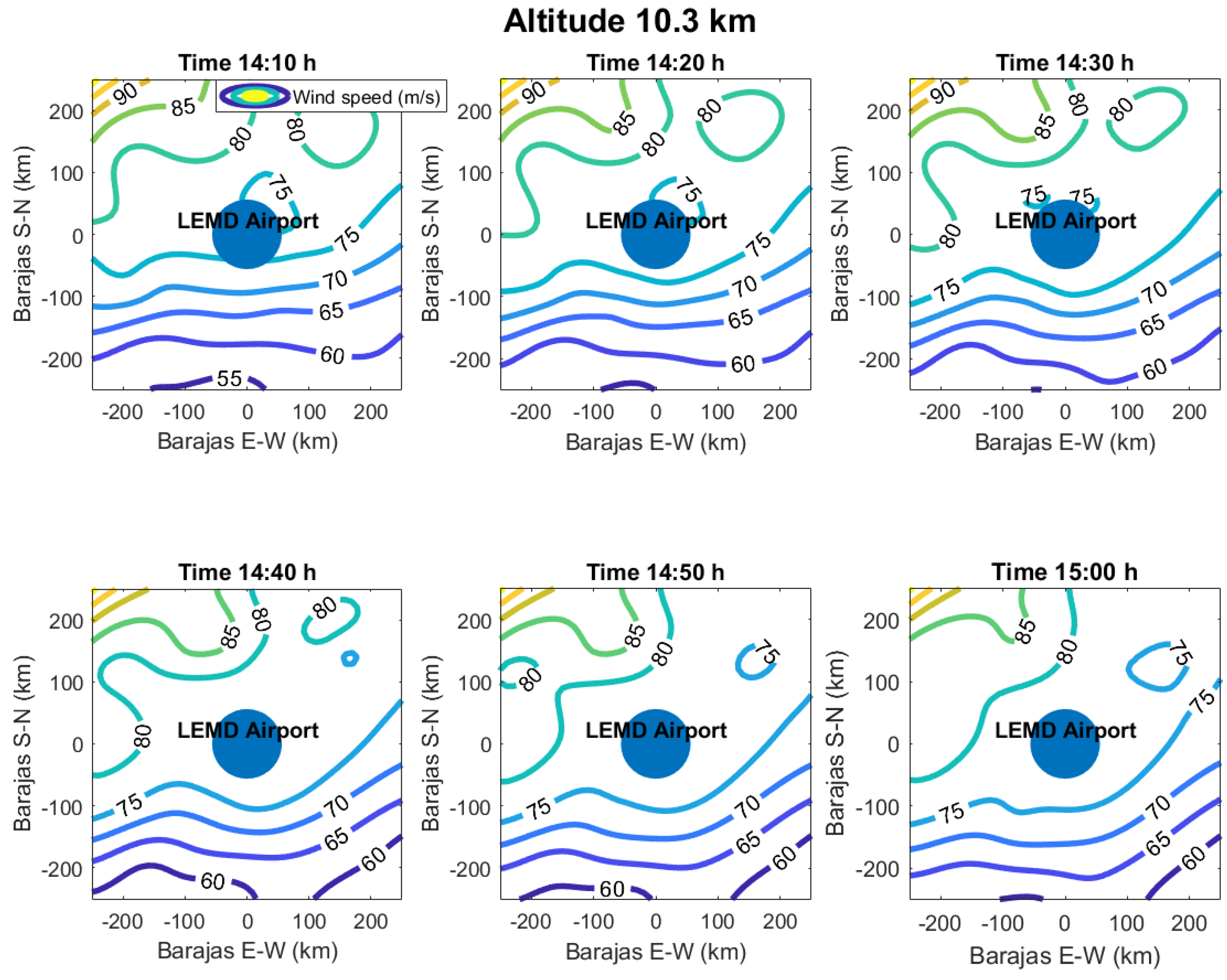
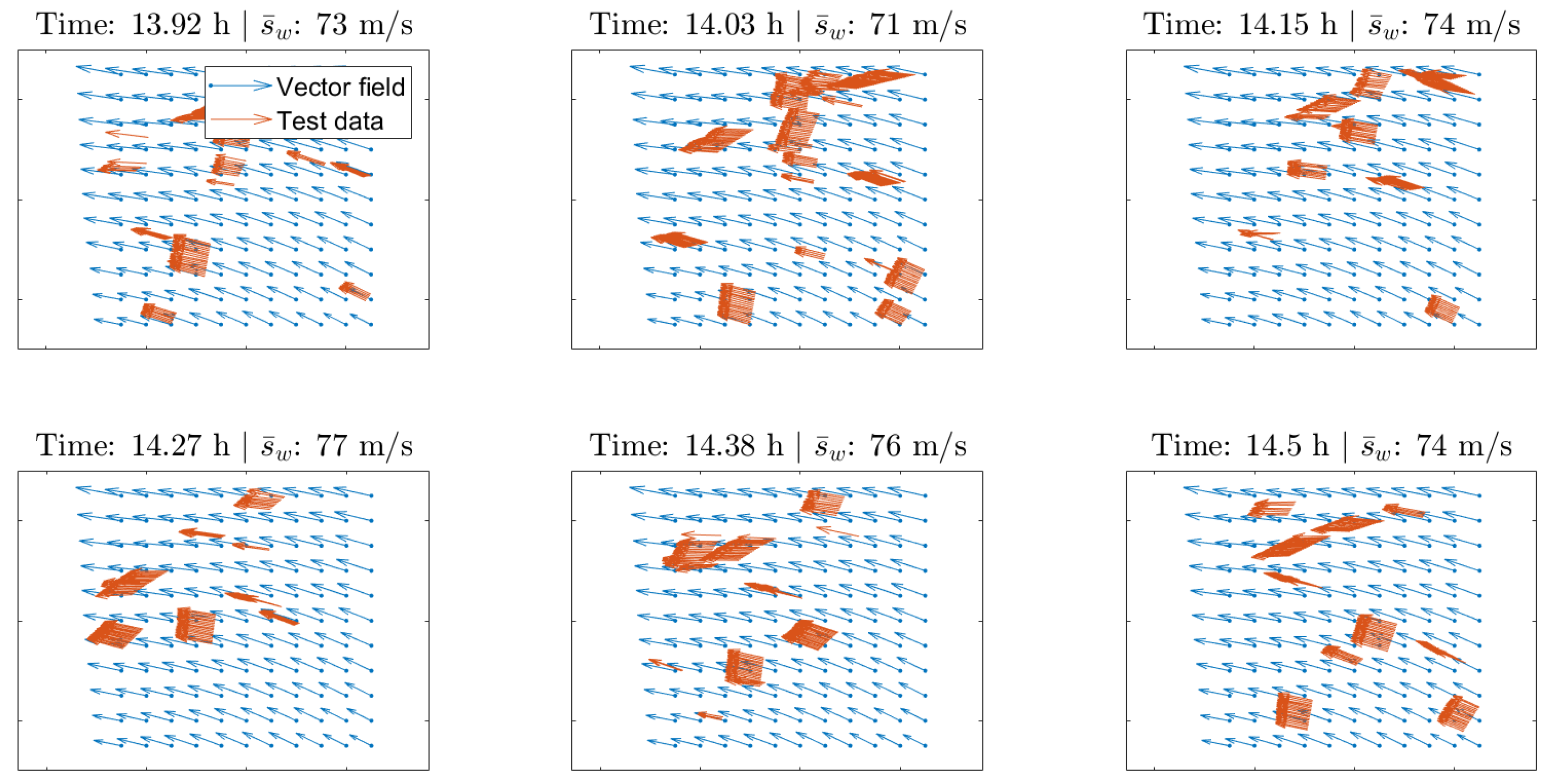
3.3. Wind Velocity Field Short-Term Prediction

The capability of the PCE-GPR method to provide the short-term wind velocity field predictions is studied in this section. In particular, several wind velocity fields were predicted around the LEMD airport using the two data sets introduced in Section 2.1.1. Each of these short time horizon predictions consists of a 15 min ahead forecast, in which the PCE-GPR model was trained using data from the previous hour and the corresponding prediction was compared to the test data available at this short time horizon. The estimation errors of these predictions were collected and aggregated. More specifically, the RMSE, the MAE, and the MAD were computed and are summarized in

Table 3. Wind velocity field prediction: Estimation errors for the u and v components of the wind velocity field.

Measure of Error	Component	Day 1	Day 2
RMSE (m/s)	u	5.28 (6%)	6.37 (13%)
	v	5.16 (6%)	5.80 (8%)
MAE (m/s)	u	4.00 (12%)	4.19 (29%)
	v	3.93 (12%)	4.40 (15%)
MAD (m/s)	u	3.00 (4%)	3.25 (12%)
	v	3.07 (3%)	3.52 (4%)

.

It can be observed that the magnitude of the estimation errors shown in Table 3 for the wind velocity field prediction is similar to the magnitude of the estimation errors reported in Table 2 for the wind velocity field reconstruction using the data sets randomly split by flight. This higher value of the estimation uncertainty with respect to the wind velocity field reconstruction using the data sets randomly split by observation is due to the fact that, unlike the PCE-GPR reconstruction model, the PCE-GPR prediction model solely relies on past observations of the wind velocity.

Table 3 also reports, between parentheses, the relative improvement obtained in comparison with the values of the estimation errors reported in [20], in which the wind velocity field prediction was carried out using the GPR method without the improvement provided by the PCE. It can be seen that, for all error measures, the PCE-GPR method outperforms the GPR method. Therefore, the PCE-GPR model yields better short-term forecasts than those provided by the GPR model, which already provided short-term predictions with reasonable estimation errors.

Figure 8 presents the wind velocity field prediction at cruise altitude obtained using the Day 2 data set and the PCE-GPR method for different instants in time. In addition, some of the members of the test data sets along with the mean wind speed at each instant in time are also shown. It can be seen that the predicted wind velocity fields largely agree with the observations.

3.4. Validation of the PCE-GPR Model

This section presents the validation of the PCE-GPR model. More specifically, the obtained estimates are compared with the observations available in the ECMWF ERA5 reanalysis database, which contains global atmospheric reanalysis data for each altitude level with a resolution of 0.25 degrees in the latitude and longitude.

In order to assess whether the aircraft-derived data agree with the reanalysis data, a comparison between the aircraft-derived data and the ECMWF ERA5 data was carried out in [20]. The differences between the aircraft-derived data and the reanalysis data were calculated for each hour ranging between 09:00 and 15:00 UTC, with a time gap of 15 min and an altitude difference of 1000 ft. Since the ECMWF ERA5 data are provided at the grid points, a linear interpolation was used to compute the reanalysis observations corresponding to the locations at which aircraft-derived observations were available. It can be seen in ([20], Table 4) that, for both the Day 1 and Day 2 data sets, the wind speed bias is less than 3 m/s, whereas the wind direction bias is less than 4 degrees. Moreover, the MAE of the wind speed is similar for both data sets, whereas the dispersion in the wind direction is significantly higher for the Day 1 data set. However, despite the difference, it is expected that the estimates provided by the PCE-GPR model agree on average with the reanalysis data.

The following steps were performed to compare the estimates of the PCE-GPR method with the ECMWF ERA5 reanalysis data. First, the reanalysis data corresponding to the Day 1 and Day 2 data sets were extracted from the ECMWF ERA5 database. Various instants in time and altitudes were considered for each data set. More precisely, the ECMWF ERA5 reanalysis data for altitudes of 5.6, 9.3, 10.5, 11.2, 12, and 12.9 km, corresponding to times 09:00, 12:00, and 15:00 UTC were considered. A cuboidal space centered at the LEMD airport with base size $500\times 500$ km was used to represent the relevant airspace. Then, the PCE-GPR model was trained on the aircraft-derived data observed in the relevant airspace and an estimation was performed at every grid point of the ECMWF ERA5 data set. The obtained estimates were compared with the ECMWF ERA5 reanalysis observations. Finally, several measures of error were calculated.

The comparison between the estimates of the wind speed and the wind direction computed using the PCE-GPR technique and the ECMWF ERA5 observations, for both the Day 1 and Day 2 data sets, are shown in

Table 4. Validation of the PCE-GPR model: Comparison between the estimates obtained using the PCE-GPR method and the ECMWF ERA5 reanalysis data.

Measure	Variable	Day 1	Day 2
Bias (m/s)	Wind speed	−2.75	−0.24
MAE (m/s)	Wind speed	4.5	5.79
Bias (deg)	Wind direction	2.06	−1.36
Dispersion (%)	Wind direction	8.5	0.33

. It can be seen that all the measures are even smaller than those reported in ([20], Table 4), except for the MAE of the wind speed for the Day 2 data set, which is almost the same. This is because the wind velocity field estimates provided by using the PCE-GPR method are smoother than the aircraft-derived data, which contain noise. Since the measurement noise $\epsilon$ is incorporated into the model (2), the PCE-GPR acts as a noise filter.

Notice that most of the aircraft-derived observations are located at cruise altitudes close to the LEMD airport. Nevertheless, the estimates provided by using the PCE-GPR model are also similar to the reanalysis data when the aircraft-derived observations near the ECMWF ERA5 grid points are not available, which shows the ability of the PCE-GPR method to yield reasonable wind velocity field estimations.

4. Discussion

Aircraft-derived wind velocity data employed in this article were supplied by ENAIRE. Specifically, they were extracted from the ASTERIX database. The wind velocity was indirectly obtained from the state of the aircraft. An exploratory analysis of the data can be found in [20], where it was observed that the noise in the wind speed increases in the data collected during aircraft turning maneuvers. The data availability and quality are expected to increase after the deployment of the European System-Wide Information Management (SWIM), an ongoing European project [43,44], which consists of a unified infrastructure to exchange the flight information, including the wind velocity directly measured by the aircraft.

The method proposed in this article was tested in different wind scenarios and different training-test data configurations. Specifically, two sets of data collected on two different days with different wind intensities and directions were selected. Each data set was randomly split in two different ways, namely by observation and by flight.

The method was tested first in the wind vector field reconstruction using both data sets. The performance of the method in terms of errors is similar. In particular, as expected, the data set configuration obtained by randomly splitting the data set by flight led to the worst wind vector field reconstruction errors in comparison to the data set configuration obtained by randomly splitting the data set by observation because, in the first case, the observations are less evenly distributed in space. However, in all training-test data configurations, these errors are unbiased and have little dispersion. Therefore, it can be concluded that the method is not affected by the wind scenario in wind vector field reconstruction.

The proposed method has also been tested in wind vector field short-term prediction using both data sets. The performance of the method, in terms of errors, is again similar. The prediction errors are higher than the reconstruction errors using the data set configuration obtained by randomly splitting the data set by observation but are similar to the reconstruction errors using the data set configuration obtained by randomly splitting the data set by flight. Therefore, it can be concluded that the errors in the short-term wind velocity field prediction are reasonably small, given that wind velocity information is only based on the past observations and therefore carries a higher level of uncertainty compared to wind velocity field reconstruction.

The performance in terms of the estimation errors of the method proposed in this paper was compared with that of the Gaussian process regression method presented by the same authors in [20]. The results demonstrate that the good performance of the previous method was further improved. Moreover, the obtained estimates were validated using an external data set, namely the ECMWF ERA5 reanalysis data, which are a reliable collection of historical atmospheric data. This comparison has shown that there is consistency between the obtained estimates and the ECMWF ERA5 reanalysis data, including the regions in which the aircraft-derived data broadcasting is low or nonexistent.

5. Conclusions

In this paper, a technique for short-term wind velocity field forecasting and wind velocity field reconstruction using aircraft-derived wind velocity data was presented. The wind velocity data were obtained in an indirect way from the states of the aircraft transmitted by the ADS-B and Mode-S aircraft surveillance systems. The amount of wind velocity data derived from aircraft states continuously transmitted airborne is large, causing these aircraft surveillance systems to be a suitable source for data assimilation algorithms. The proposed technique combines the Gaussian process regression method with the arbitrary polynomial chaos expansion, which causes the Gaussian process regression to be more precise since it models the mean spatiotemporal behavior of the wind through polynomial functions rather than linear functions.

The main advantages of the method are that it does not rely on spatial and temporal grids and that new observations can be assimilated in less than 5 min, causing it to be suitable for short-term forecasting. The ultimate goal of the method presented in this article is to increase aircraft trajectory predictability in TBO, which is an operational concept that is expected to be implemented soon [45].

Future research will concentrate on showing the advantages of the improved wind velocity information obtained through the method described in this paper on the predictability of aircraft trajectories in the TBO framework. These advantages have already been demonstrated in some articles, such as [2], where the optimal descent trajectory is updated in real-time using wind velocity profiles, and [12], where KF-based wind velocity profiles are used for reducing the temporal spacing error between aircraft.

References

1. Hernández-Romero, E.; Valenzuela, A.; Rivas, D. Probabilistic multi-aircraft conflict detection and resolution considering wind forecast uncertainty. Aerosp. Sci. Technol. 2020, 105, 105973. [Google Scholar] [CrossRef]
2. Dalmau, R.; Prats, X.; Baxley, B. Using broadcast wind observations to update the optimal descent trajectory in real-time. J. Air Transp. 2020, 28, 82–92. [Google Scholar] [CrossRef]
3. Reynolds, T.G.; McPartland, M. Establishing wind information needs for four dimensional trajectory-based operations. In Proceedings of the 1st International Conference on Interdisciplinary Science for Innovative Air Traffic Management, Daytona Beach, FL, USA, 25–27 June 2012. [Google Scholar]
4. Reynolds, T.G.; McPartland, M.; Teller, T.; Troxel, S. Exploring wind information requirements for four dimensional trajectory-based operations. In Proceedings of the 11th USA/Europe Air Traffic Management Research and Development Seminar, Lisbon, Portugal, 23–26 June 2015. [Google Scholar]
5. de Haan, S. High-resolution wind and temperature observations from aircraft tracked by Mode-S air traffic control radar. J. Geophys. Res. Atmos. 2011, 116, D10111. [Google Scholar] [CrossRef]
6. Sun, J.; Vû, H.; Ellerbroek, J.; Hoekstra, J.M. pyModeS: Decoding Mode-S surveillance data for open air transportation research. IEEE Trans. Intell. Transp. Syst. 2020, 21, 2777–2786. [Google Scholar] [CrossRef]
7. Sun, J. The 1090 Megahertz Riddle: A Guide to Decoding Mode S and ADS-B Signals; TU Delft OPEN Publishing: Delft, The Netherlands, 2021. [Google Scholar]
8. Guzzi, R. Data Assimilation: Mathematical Concepts and Instructive Examples; Springer: Cham, Switzerland, 2016. [Google Scholar]
9. de Haan, S.; Stoffelen, A. Assimilation of high-resolution Mode-S wind and temperature observations in a regional NWP model for nowcasting applications. Weather Forecast. 2012, 27, 918–937. [Google Scholar] [CrossRef]
10. Cardinali, C.; Isaksen, L.; Andersson, E. Use and impact of automated aircraft data in a global 4DVAR data assimilation system. Mon. Weather Rev. 2003, 131, 1865–1877. [Google Scholar] [CrossRef]
11. Talagrand, O. Assimilation of observations, an introduction. J. Meteorol. Soc. Jpn. 1997, 75, 191–209. [Google Scholar] [CrossRef] [Green Version]
12. de Jong, P.M.A.; van der Laan, J.J.; in ’t Veld, A.C.; van Paassen, M.M.; Mulder, M. Wind-profile estimation using airborne sensors. J. Aircr. 2014, 51, 1852–1863. [Google Scholar] [CrossRef]
13. Liu, T.; Xiong, T.; Thomas, L.; Liang, Y. ADS-B based wind speed vector inversion algorithm. IEEE Access 2020, 8, 150186–150198. [Google Scholar] [CrossRef]
14. Dalmau, R.; Pérez-Batlle, M.; Prats, X. Estimation and prediction of weather variables from surveillance data using spatio-temporal Kriging. In Proceedings of the 2017 IEEE/AIAA 36th Digital Avionics Systems Conference, St., Petersburg, FL, USA, 17–21 September 2017. [Google Scholar]
15. Sun, J.; Vû, H.; Ellerbroek, J.; Hoekstra, J.M. Weather field reconstruction using aircraft surveillance data and a novel meteo-particle model. PLoS ONE 2018, 13, e0205029. [Google Scholar] [CrossRef]
16. Zhu, J.; Wang, H.; Li, J.; Xu, Z. Research and optimization of meteo-particle model for wind retrieval. Atmosphere 2021, 12, 1114. [Google Scholar] [CrossRef]
17. Enea, G.; McPartland, M. Wind enhancements for trajectory based operations automation. In Proceedings of the AIAA Aviation 2022 Forum, Chicago, IL, USA, 27 June–1 July 2022. [Google Scholar]
18. Marinescu, M.; Olivares, A.; Staffetti, E.; Sun, J. Wind profile estimation from aircraft derived data using Kalman filters and Gaussian process regression. In Proceedings of the 14th USA/Europe ATM Research and Development Seminar, Virtual Event, 20–23 September 2021. [Google Scholar]
19. Marinescu, M.; Olivares, A.; Staffetti, E.; Sun, J. On the estimation of vector wind profiles using aircraft-derived data and Gaussian process regression. Aerospace 2022, 9, 377. [Google Scholar] [CrossRef]
20. Marinescu, M.; Olivares, A.; Staffetti, E.; Sun, J. Wind field estimation from aircraft derived data using Gaussian process regression. PLoS ONE 2022, 17, e0276185. [Google Scholar] [CrossRef] [PubMed]
21. Wiener, N. The homogeneous chaos. Am. J. Math. 1938, 60, 897–936. [Google Scholar] [CrossRef]
22. Xiu, D.; Karniadakis, G.E. The Wiener-Askey polynomial chaos for stochastic differential equations. SIAM J. Sci. Comput. 2002, 24, 619–644. [Google Scholar] [CrossRef]
23. Oladyshkin, S.; Nowak, W. Data-driven uncertainty quantification using the arbitrary polynomial chaos expansion. Reliab. Eng. Syst. Saf. 2012, 106, 179–190. [Google Scholar] [CrossRef]
24. Schöbi, R.; Sudret, B.; Wiart, J. Polynomial-chaos-based Kriging. Int. J. Uncertain. Quantif. 2015, 5, 171–193. [Google Scholar] [CrossRef] [Green Version]
25. Schöbi, R.; Sudret, B.; Marelli, S. Rare event estimation using polynomial-chaos Kriging. ASCE-ASME J. Risk Uncertain. Eng. Syst. Part A Civ. Eng. 2017, 3, D4016002. [Google Scholar] [CrossRef] [Green Version]
26. Martino, L.; Read, J. A joint introduction to Gaussian processes and relevance vector machines with connections to Kalman filtering and other kernel smoothers. Inf. Fusion 2021, 74, 17–38. [Google Scholar] [CrossRef]
27. ASTERIX Official Web Page. Available online: https://www.eurocontrol.int/asterix (accessed on 15 November 2022).
28. EUROCONTROL Technical Document Part12-CAT021. Available online: https://www.eurocontrol.int/publication/cat021-eurocontrol-specification-surveillance-data-exchange-asterix-part-12-category-21 (accessed on 15 November 2022).
29. EUROCONTROL Technical Document Part04-CAT048. Available online: https://www.eurocontrol.int/publication/cat048-eurocontrol-specification-surveillance-data-exchange-asterix-part4 (accessed on 15 November 2022).
30. Jammalamadaka, S.R.; Sengupta, A. Topics in Circular Statistics; World Scientific Publishing: Singapore, 2001. [Google Scholar]
31. Rasmussen, C.E.; Williams, C. Gaussian Processes for Machine Learning; MIT Press: Cambridge, MA, USA, 2006. [Google Scholar]
32. Shi, J.Q.; Choi, T. Gaussian Process Regression Analysis for Functional Data; Chapman and Hall: London, UK, 2011. [Google Scholar]
33. Torre, E.; Marelli, S.; Embrechts, P.; Sudret, B. Data-driven polynomial chaos expansion for machine learning regression. J. Comput. Phys. 2019, 388, 601–623. [Google Scholar] [CrossRef] [Green Version]
34. Wan, X.; Karniadakis, G.E. Beyond Wiener-Askey expansions: Handling arbitrary PDFs. J. Sci. Comput. 2006, 27, 455–464. [Google Scholar] [CrossRef] [Green Version]
35. Oladyshkin, S.; Nowak, W. Incomplete statistical information limits the utility of high-order polynomial chaos expansions. Reliab. Eng. Syst. Saf. 2018, 169, 137–148. [Google Scholar] [CrossRef]
36. Gramacki, A. Nonparametric Kernel Density Estimation and Its Computational Aspects; Springer: Cham, Switzerland, 2018. [Google Scholar]
37. Silverman, B.W. Density Estimation for Statistics and Data Analysis; Chapman and Hall: London, UK, 1986. [Google Scholar]
38. The Modified Rastrigin Function. Available online: https://uqworld.org/t/modified-rastrigin-function/126 (accessed on 15 November 2022).
39. Wang, B.; Chen, T. Gaussian process regression with multiple response variables. Chemom. Intell. Lab. Syst. 2015, 142, 159–165. [Google Scholar] [CrossRef] [Green Version]
40. Stein, M.L. The loss of efficiency in Kriging prediction caused by misspecifications of the covariance structure. Geostatistics 1989, 4, 273–282. [Google Scholar]
41. Micchelli, C.A.; Xu, Y.; Zhang, H. Universal kernels. J. Mach. Learn. Res. 2006, 7, 2651–2667. [Google Scholar]
42. Bo, L.; Sminchisescu, C. Greedy block coordinate descent for large scale Gaussian process regression. In Proceedings of the Proceedings of the Twenty-Fourth Conference on Uncertainty in Artificial Intelligence, Helsinki, Finland, 9–12 July 2008. [Google Scholar]
43. Masutti, A. Single European sky—A possible regulatory framework for System Wide Information Management (SWIM). Air Space Law 2011, 36, 275–292. [Google Scholar] [CrossRef]
44. SWIM Project. Available online: https://www.eurocontrol.int/concept/system-wide-information-management (accessed on 15 November 2022).
45. AIRBUS: 4D-TBO. Available online: https://www.airbus.com/en/newsroom/stories/2020-12-4d-tbo-a-new-approach-to-aircraft-trajectory-prediction (accessed on 15 November 2022).
Figure 1. Relationship among the true airspeed, ground speed, and wind velocity vectors.
Mathematics 11 01018 g001
Figure 2. Aircraft flight routes for the Day 1 data set.
Mathematics 11 01018 g002
Figure 3. The Rastrigin function and its approximation by the GPR, PCE, and PCE-GPR models.
Mathematics 11 01018 g003
Figure 4. Rose diagrams of the wind velocity estimation errors.
Mathematics 11 01018 g004
Figure 5. Wind velocity field reconstruction: Reconstructed wind velocity field obtained using the Day 1 data set and the PCE-GPR method for different altitudes (A). A selection of members of the training and test data sets, along with the mean wind speed ( s ¯ w ), are also included.
Mathematics 11 01018 g005
Figure 6. Rose diagrams of the wind velocity estimation errors, segmented by altitude, for the Day 1 data set split by flight.
Mathematics 11 01018 g006
Figure 7. Wind speed reconstruction from 14:10 to 15:00 UTC at cruise altitude for the Day 2 data set.
Mathematics 11 01018 g007
Figure 8. Wind velocity field prediction: Predicted wind velocity field at cruise altitude obtained using the Day 2 data set and the PCE-GPR method for different instants in time. A selection of members of the test data sets, along with the mean wind speed ( s ¯ w ), are also included.
Mathematics 11 01018 g008