Article

Efficient Net-XGBoost: An Implementation for Facial Emotion Recognition Using Transfer Learning

by
Sudheer Babu Punuri
1,
Sanjay Kumar Kuanar
1,
Manjur Kolhar
2,*,
Tusar Kanti Mishra
3,*,
Abdalla Alameen
4,
Hitesh Mohapatra
5 and
Soumya Ranjan Mishra
5
1
CSE Department, GIET University, Gunupur 765022, Odisha, India
2
Department of Computer Science, College of Arts and Science, Prince Sattam Bin Abdulaziz University, Al-Kharj 16278, Saudi Arabia
3
School of Computer Science and Engineering, Vellore Institute of Technology, Vellore 632014, Tamil Nadu, India
4
Computer Science Department, Prince Sattam Bin Abdul Aziz University, Al-Kharj 16278, Saudi Arabia
5
School of Computer Engineering, KIIT (Deemed to Be) University, Bhubaneswar 751024, Odisha, India
*
Authors to whom correspondence should be addressed.
Mathematics 2023, 11(3), 776; https://doi.org/10.3390/math11030776
Submission received: 29 December 2022 / Revised: 14 January 2023 / Accepted: 29 January 2023 / Published: 3 February 2023
(This article belongs to the Special Issue Fuzzy Logic and Computational Intelligence)

Abstract

:
Researchers are interested in Facial Emotion Recognition (FER) because it could be useful in many ways and has promising applications. The main task of FER is to identify and recognize the original facial expressions of users from digital inputs. Feature extraction and emotion recognition make up the majority of the traditional FER. Deep Neural Networks, specifically Convolutional Neural Network (CNN), are popular and highly used in FER due to their inherent image feature extraction process. This work presents a novel method dubbed as EfficientNet-XGBoost that is based on Transfer Learning (TL) technique. EfficientNet-XGBoost is basically a cascading of the EfficientNet and the XGBoost techniques along with certain enhancements by experimentation that reflects the novelty of the work. To ensure faster learning of the network and to overcome the vanishing gradient problem, our model incorporates fully connected layers of global average pooling, dropout and dense. EfficientNet is fine-tuned by replacing the upper dense layer(s) and cascading the XGBoost classifier making it suitable for FER. Feature map visualization is carried out that reveals the reduction in the size of feature vectors. The proposed method is well-validated on benchmark datasets such as CK+, KDEF, JAFFE, and FER2013. To overcome the issue of data imbalance, in some of the datasets namely CK+ and FER2013, we augmented data artificially through geometric transformation techniques. The proposed method is implemented individually on these datasets and corresponding results are recorded for performance analysis. The performance is computed with the help of several metrics like precision, recall and F1 measure. Comparative analysis with competent schemes are carried out on the same sample data sets separately. Irrespective of the nature of the datasets, the proposed scheme outperforms the rest with overall rates of accuracy being 100%, 98% and 98% for the first three datasets respectively. However, for the FER2013 datasets, efficiency is less promisingly observed in support of the proposed work.

1. Introduction

Facial Emotion Recognition (FER) techniques are used to identify facial expressions that convey emotions on human faces. Different types of emotions exist, some of which might not be apparent to the human eye. Hence, with proper tools, any indications preceding or following can be related to identifying the recognition [1]. In the field of FER, there are seven universal facial expressions namely: anger, fear, disgust, happiness, sadness, surprise, and neutral. Emotion extraction from facial expressions is a topic of active research in psychology, psychiatry, and mental health at present. The automatic detection of emotions from facial expressions has many uses, including smart living, health care, HCI (human-computer interaction), HBI (human-robot interaction), and modern augmented reality [2]. Researchers keep looking into FER because it has so many uses.
The main goal of FER is to match different facial expressions with different emotional states. In the classical FER, the two most important steps are “feature extraction” and “emotion recognition”. Prior to feature extraction, all images need to be preprocessed, which includes finding faces, cropping, resizing, and normalising. Standard techniques which includes notable methods such as discrete wavelet transform and histogram of oriented gradients (HOG) [3] are suitably used for feature extraction. Finally, neural networks (NN) and other machine learning techniques are used to classify emotions based on the features that were extracted.
Deep neural networks (DNNs), especially convolutional neural networks (CNNs), are popular among researchers working on FER. This is because of the inherent feature extraction and recognition integration architectures [4,5,6]. However, the current FER approaches reported by CNN still have some challenges. The very low difference in facial expressions due to different emotional states makes the task challenging. Further, substantial intra-class variance and low inter-class variation [7] along with changes in facial position have also posed several challenges. Challenges also persist in emotion recognition under naturalistic situations like occlusion and pose variation [8], which can dramatically alter facial appearance. This is where we try to identify an opportunity for research. Advances in computer vision [9] has lead to high-quality emotion recognition under controlled conditions and consistent environments.
Nowadays, the applications of deep learning, particularly CNN, make it possible to extract numerous features and learn from them. A CNN with several hidden layers requires difficult training and performs poorly in practice. In order to improve accuracy, deep CNN architecture can be pre-trained using a variety of models and methodologies. EfficientNet [10], DenseNet-161 [1], Inception-v3, Resnet-50, and VGG-16 [1] are the most popular pre-trained DCNN models; however, training a large model takes a huge dataset and intensive computing power.
Advanced computer vision research, is also able to solve the problem of unlabeled data, in medical image analysis. Moreover, there is no guarantee of large datasets for training. Ref. [11]’s work has solved the problem of unlabeled data and developed an estimation method for hard cases. As the volume of the dataset grows, we require high computing power. This situation is resource hunger. GPUs are a must for computing large datasets. For efficiently Using GPUs, we need to accelerate. Mengyang Zhao et al. [12] contribute a novel method for GPU acceleration by a method fast mean shift algorithm, which increases speed by up to 7–10 times. Face recognition has a wide range of applications. Capturing devices may produce 2D images, but there is a need for 3D images for more spatial information. Jin, B [13] have introduced the D+GAN method for the translation of image-to-image with facial conditions.
Training a deep learning model from scratch requires a lot of processing power and takes a long time. As a result, rather than reinventing the wheel, a Deep Convolutional Neural Network (DCNN) trained on another task and fine-tuned can be used. This approach is called “Transfer Learning” (TL) [14]. The conditions required for applying transfer learning are data type consistency and similarity in the problem domain. In our study EfficientNet [10], already pre-trained on a large dataset of imagenet is used for the task of FER. CNN’s are scaled up to achieve better accuracy in the task of classification on most benchmark datasets. But convolutional techniques of model scaling are done randomly. Some models are scaled depth-wise and others width-wise. Random scaling requires manual tuning and requires many person-hours. EfficientNet on the other hand, uses a method called “compound co-efficient” to scale models in a simple but effective way. After extraction of features using pre-trained DCNN models, efficient classification models can be employed for the task of emotion recognition. XGBoost [15] is an algorithm under the category of supervised learning. This algorithm runs on both single and distributed systems for classifying the input samples. In case of large data sets, XGBoost does efficient memory management keeping the limitations of the RAM size and supports cross validation. It also has a wide range of regularizations, which helps with the reduction of overfitting. Through auto tree pruning it avoids decision tree growth after a certain limit internally. This motivates us to take-up XGBoost as a classifier in our research pipeline. This study’s key contribution can be summed up as follows:
(i)
To implement a robust FER technique utilising the power of Transfer Learning through EfficientNet-XGBoost model.
(ii)
Adding fully connected layers to the model for fine tuning for attaining high accuracy.
(iii)
Analyze the proposed method’s proficiency by comparing its accuracy in recognising emotions to that of other methods currently in use.

2. Related Work

In recent times, several techniques have been proposed in the context of FER. According to conventional methods, facial features are extracted first, and emotions are then classified using those features. On the other hand, the FER job is done by current deep-learning models that combine both steps into a single computational process.
In the domain of artificial intelligence (AI) domain, automatic FER has become a challenging task, mostly in its subdomain of Machine Learning (ML). FER was implemented using different traditional algorithms like K-Nearest Neighbor (KNN), neural networks, etc. during the origin of FER. The methods like wavelet energy feature (WEF) and Fisher’s linear discriminants (FLD) were the first methods used for feature extraction, and the KNN method is used for classifying the classes of emotions. Feng et al. [16] extracted the Local Binary Patterns (LBP) histograms from images at different locations, summed all these patterns, and then classified the emotion using a linear programming (LP) technique. Lee et al. [1] improved the wavelet transform for 2D, named contourlet transform (CT), in order to extract features from images and used boosting algorithms for classifying emotions. Support vector machine (SVM) is used by various models for classification of emotions for the extracted features using different techniques. Liew adn Yairi [17] have done a comparative study considering SVM and several other methods, which include Gabor, Haar, and LBP. Two years ago, researchers found various classification algorithms for their suggested geometry-based feature extraction, including logistic regression, LDA (linear discriminate analysis), examples include KNN, naive Bayes, SVM, and classification and regression trees. Goodfellow et al. [3] FER2013 dataset is used to construct a model on FER, although it could only reach 57.7% accuracy using the Histogram of Oriented Gradients (HOG) feature extractor and SVM. This is much worse accuracy than the baseline. The primary drawback of these conventional methods is that they only consider the frontal views of FER as features.
A new approach for FER is deep learning in machine learning, and so far there are several CNN-based models introduced in the literature. The integration of deep belief network (DBN) and neural network (NN) was proposed by Zhao and Shi [18], where DBN is used for feature extraction and the neural network is used for classifying emotions. At first, some models used a standard CNN architecture with two convolutional-pooling layers to look at the images of facial expressions of emotion that they had collected for FER. Mollahosseini et al. [19] introduced a bigger model with 4-inception and 2-convolutional-pooling layers. Pons and Masipcite [4] developed an ensemble of 72 CNNs, where each CNN is trained on different filter sizes in convolutional layers and a different number of neurons in fully connected layers. The [5] model also employs an ensemble of 100 CNNs, whereas the previous model utilised a predetermined number of CNNs. When all of the FER datasets were benchmarked, CNN-based deep learning models had the highest accuracy. However, unlike HOG or LBP, existing models implement the recognition process as a whole. Image classification applications were used by combining CNN model using KNN or the SVM classifier, which attained slightly higher accuracy than CNN models. Jabid et al. [6] and Shima and Omori [20] fine-tuned the algorithm and improved better accuracy on the dataset JAFFE by 90.1% and 95.3% respectively. With 35,887 images, the FER-2013 dataset is the most challenging one. Saeed et al. [21] achieved a baseline accuracy of 68 percent.
Xiao Sun and Man Lv [22] created a model with hybrid features that combine SIFT and deep learning features using a CNN model with different levels of extraction. Ref. [23] proposed a multilevel Haar wavelet-based approach. By using the Viola-Jones cascade, object detector components like eyes, mouths, and eyebrows are extracted. Kuan Li and Yi Jin [24] proposed a cropping and rotation method which makes the model easy to train only on the useful features. C. Shi, CTan et al. [25] proposed a model that effectively extracts features by modifying the structure of a single CNN model based on a Multi-Branch Cross-Connection (MBCC-CNN). M. Aouayeb et al. [26] developed a model with Squeeze and Excitation with Vision Transformer which overcomes the disadvantages of regular CNN models. Shervin et al. [2] implemented an approach using attentional convolutional networks by focusing only on the significant parts of the face images. SL Happy et al. [27] developed a model, by identifying facial patches that are active in particular emotions, thus these features are classified. [28] The authors created an automatic FER by identifying the best feature descriptor using the Facial Landmarks descriptor and classifying with Support Vector Machine (SVM). Due to ambiguity facial gestures, less-informative facial images, and subjectivity of annotators, it is enormously hard to annotate a qualitative large-scale facial expression dataset. These uncertainties pose a significant obstacle of FER in large-scale in the era of deep learning. The work of the researcher [29] proposes a simple yet effective SelfCure Network (SCN) that efficiently suppresses uncertainties and prevents deep neural networks from overfitting uncertain facial images.
Training a large neural model such as deep convolutional neural network is difficult due to the network’s numerous parameters. It is common knowledge that a large network is required to train large amounts of data. If trained with too little or insufficient data, overfitting is inevitable. In some research works, it has become a combustion task arrange sufficient sample set to train on deep convolutional neural network. However, in cases where a huge amount of data is not available, transfer learning [14,30] solves the issue. No doubt, transfer learning is a concept used to represent the knowledge learned from different tasks which has the same applications. In the literature review, it was identified that the TL method worked better when both the tasks were similar. It has been investigated that TL achieved good accuracy on the task different from training, which is the motivation of this work.

3. Materials and Methods

3.1. Deep Learning Using Transfer Learning

Reusing a model that has already been trained to solve a new issue is called transfer learning. Transfer learning has a number of advantages, but its major ones are reducing training time, improving neural network performance, and not requiring a lot of data. To the pre-trained model (EfficientNet), fully connected layers, namely global average pooling, dropout, and dense layer, are added. Lastly, to the pre-trained model, we added XGBoost for the classification.
FER is also done through pre-trained deep neural frameworks using appropriate Transfer Learning. Mahendran [30] has the learning process in frameworks such as CNN. The visualization reveals preliminary features from input images from the first layer. The next layer identifies the complex features like texture or shape. So the same mechanism goes on towards identifying the complex features. Transfer learning is primarily advantageous because it is difficult to train a DCNN from scratch. Instead of reinventing the wheel, we will use the pre-trained weights and fine-tune the model for FER. Employing TL for FER provides promising results as well.
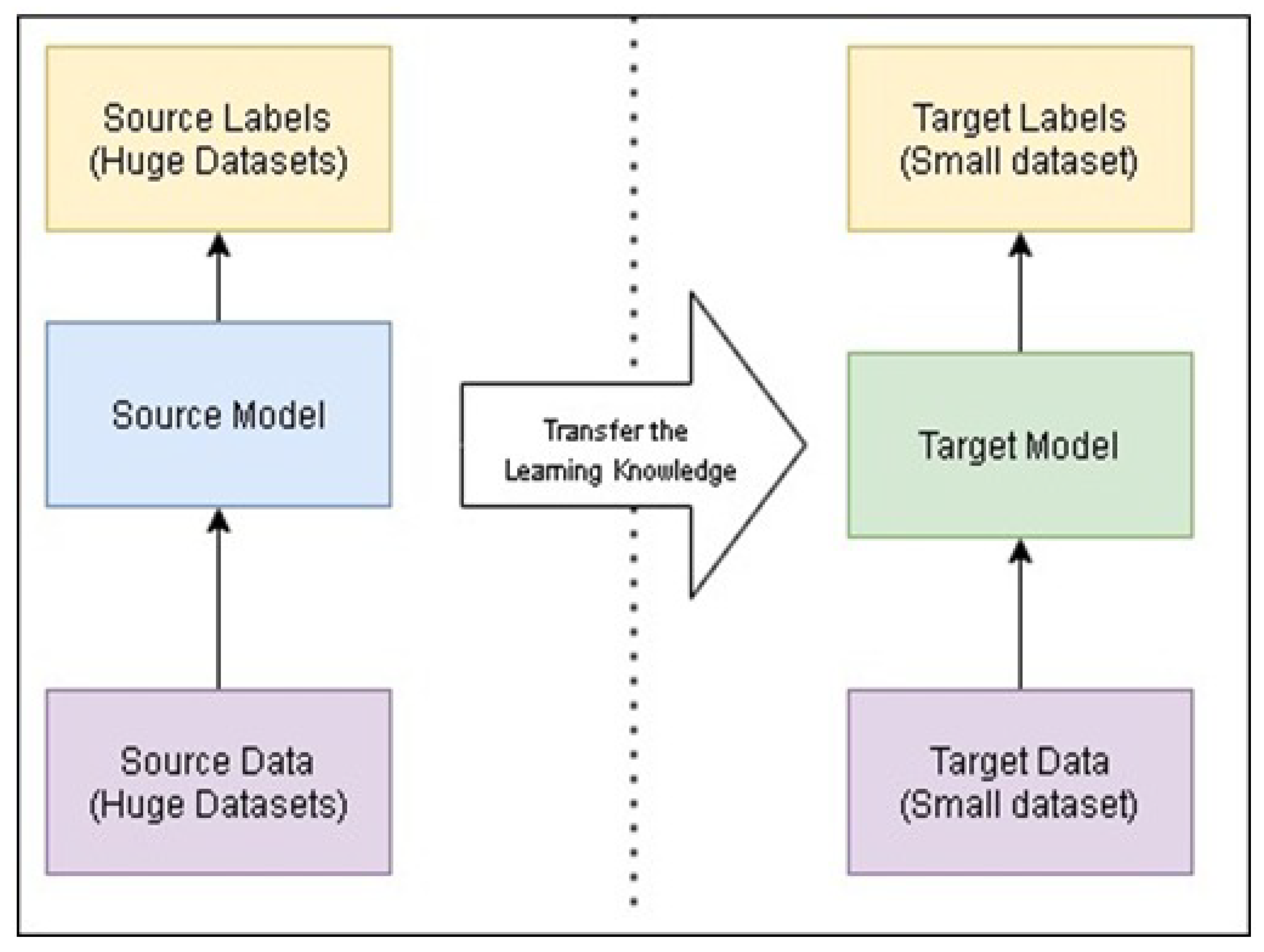
A DCNN model (EFficientNet) pre-trained with a large dataset with 1000 classes (e.g., ImageNet) is well suited for FER. Figure 1 shows the general architecture of transfer learning. Here, the foundation of the convolutional is similar to that of pre-trained DCNN by excluding the classification stage. The existing classifier part in the model is replaced by newly added fully connected layers and a classifier. Overall, the module consists of a Convolutional Base to extract feature extraction, fully connected layers for fine-tuning the model, and an XGBoost Classifier.
EfficientNets is a collection of models (named as EfficientNet-B0 to B7). They are derived by compound scaling up the baseline network EfficientNet-B0. The benefit of EfficientNets manifests itself in two ways. First, it offers high accuracy. Second, it enhances the performance of the model by reducing the dimensionality and floating-point computational cost. Compounding scaling is used to produce various versions of EfficientNet. Compound Scaling refers to the utilization of a weighted scale containing three interconnected hyperparameters of the model (stated in Equation (1)), namely depth d, width w and resolution r defined as:
d e p t h : d = A ϕ , w i d t h : w = B ϕ , r e s o l u t i o n : r = Γ ϕ
where A, B and Γ are the constants that defines the resolution of the network.
Initially, the compound coefficient is set to 1, which defines the base compound configuration, EfficientNetB0. The same configuration is used in the grid search, for optimizing the co-efficients A, B and Γ such that:
A B 2 Γ 2 2
where A ≥ 1, B≥ 1, Γ 1
We achieved the optimal values for A, B and Γ as 1.2, 1.1 and 1.15 respectively, under the constraints stated in of (2). If we change the value of in Equation (1), the scaled versions of EfficientNet-B1 to B7 will be achieved. EfficientNet-B0 baseline architecture is used for feature extraction. The EfficientNet-B0 architecture consists of mainly 3 modules, the Stem, the Blocks and the Head.
Stem: Stem has a convolutional Layer, (3 × 3) with kernel size, Batch normalization Layer, and a Swish activation. These 3 are integrated.
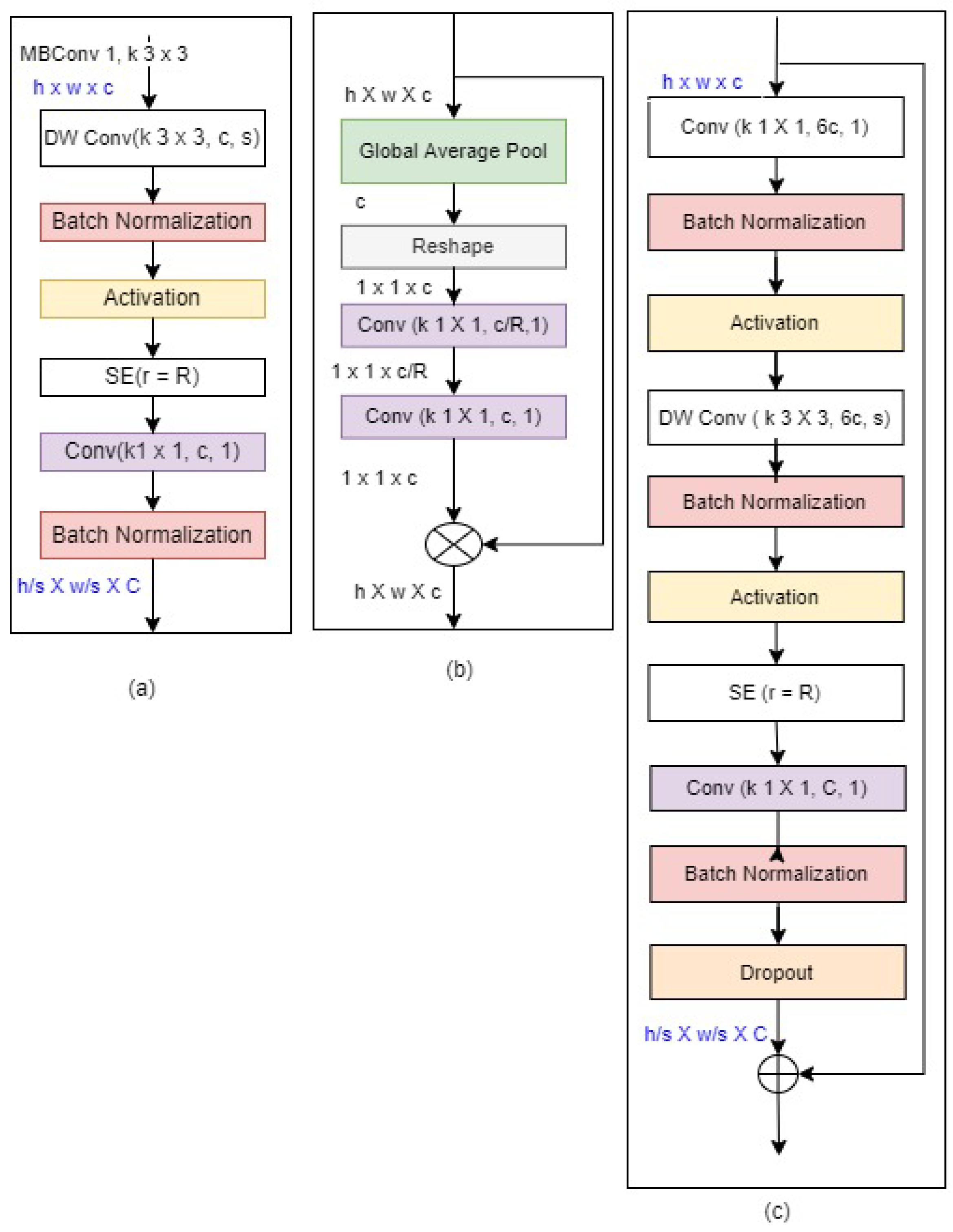
Blocks: Blocks consist of several Mobile inverted bottleneck convolutions (MBConv) Figure 2. MBConv has different versions. In MBConvX, X denotes the expansion ratio. Basically, MBConv1 and MBConv6 is used in EfficientNet. MBConv1 and MBConv6 description is given below.
M B C o n v 1 D w C + B N + S w i s h + S E + C o n v + B N
M B C o n v 6 C o n v + B N + S w i s h + D w C + B N + S w i s h + S E + C o n v + B N
where
  • DwC—DepthWise Convolution
  • BN—Batch Normalisation
  • SE—Squeeze Excitation.
  • Swish—an activation.
Figure 2. EfficientNet Blocks: (ac) are the 3 basic building blocks. h, w, and c are input with respect to height, width, and channel for all the MBConv blocks. The Output channel for the two blocks is denoted by C.
Mathematics 11 00776 g002
The no. of layers in blocks are MBConv1, k3 × 3, MBConv6, k3 × 3 repeated twice, MBConv6, k5 × 5 is repeated twice, MBConv6, k3 × 3 is repeated thrice, MBConv6, k3 × 3 is repeated thrice, MBConv6, k5 × 5 is repeated thrice, MBConv6, k5 × 5 is repeated 4 times, MBConv6, k3 × 3, total 16 blocks exists.
Head: Head is a layer consisting of Convolution, Batch Normalization, Swish, Pooling, Dropout and Fully Connected layers. Head is represented as follows:
H e a d C o n v + B N + S w i s h
The detailed EfficietNet Architecture is represented in Table 1. A Note to remember is that MBConv6, k5 × 5 and MBConv6, k3 × 3 but only the difference is that MBConv6, k5 × 5 is applied to a kernel size of 5 × 5.

3.2. Fully Connected Layer

This module consists of 3 layers Global Average Pooling, Dropout layer and Dense Layer.
Global Average Pooling: Global Average Pooling layers replace fully connected layers in traditional CNNs. In the final layer, the goal is for generating the feature sets corresponding to respective classification levels. We take the average of each feature map instead of designing a complete connected layers above the feature maps. The basic advantage of global average pooling is that it is very similar to the structure of convolutional structure by enforcing the relation between corresponding feature maps with respect to classes. Another advantage is to avoid over-fitting, as there are zero parameters to optimize in global average pooling. Global Average Pooling does something different. Average pooling is applied on. It uses average pooling on the spatial dimensions until each is one and leaves the other dimensions alone. Global Average Pooling layer does transformation of ( N 1 , N 2 , N 3 ) , feature set of size ( 1 , N 3 ) and feature map where ( N 1 , N 2 ) corresponds to image dimension, and N 3 being the count of filters used.
Dropout: While using DCNN, co-adaptation is the drawback when training a model. This indicated that the neuron are very dependent on other neurons. They influence each other considerably and are not independent enough regarding their inputs. It is very common to find in some situation that some neurons have a predictive capacity that is more significant than others. These kind of state can be avoided and the weights must be distributed to prevent over-fitting. There are various regularization methods which can be applied for regulating co-adaptation and high predictive capacity of of some neurons. To resolve this problem Dropout can be used. Depending on whether the model is DCNN, or a CNN or a Recurrent Neural Network (RNN) different dropout methods can be used. Here in our work we have used standard dropout method. The modeling of dropout layer on a neuron mathematically represented as follows:
f ( κ , ρ ) = κ if κ = 1 1 ρ if κ = 0
where:
  • κ denotes the desired results.
  • ρ is the probability of the real-valued representations.
  • If ρ = 1 the neuron holding a real value is de-activated else activated.
The next layer we have is dense layer. In the neural network, a dense layer deeply connects to its next layer. Each of the neuron links to every neuron of its next layer. The neuron in this dense layer represents the neuron’s matrix-vector multiplications. Every neuron in the dense layer unit receives output from each neuron in the preceding layers in the model. The dense layer units perform matrix-vector cross product. In product, the row vector of the output from the previous layers is identical to the column vector of the dense layer. The major hyper parameters to tune in this layer are units and activation function. The very basic and necessary parameter in dense layer is units. In dense layer, size is defined by units which is always greater than 1. Activation function aids in transforming the input values to neurons. Basically it produces non-linearity into the network where relationship of input and output values are learnt.
3.3. XGBoost

eXtreme Gradient Boosting (XGBoost) [15] algorithm is one of the best algorithm in Machine Learning (ML) developed by Chen and Guestrin. XGBoost can be considered as both a classifier and regressor in the framework of scikit-learn. The XGBoost model for classification is called XGBClassifier which is used in this study. We can create and fit to our training dataset. The beauty of XGBoost is its scalability, which drives fast learning through parallel and distributed computing and provides memory usage efficiently. XGBoost is a distributed gradient boosting library that has been developed to be highly versatile and portable. The objective function (loss function and regularization) is represented as follows:
F t j = 1 T [ ( i ϵ I j g i ) w j + 1 2 ( i ϵ I j h i + λ ) w j 2 ] + = ρ T
  • F—Objective Function
  • g i —Mean Square Error first derivative.
  • w—Score Vectors on leaves.
  • h i —Mean Square Error second derivative.
  • λ —Penality
  • T—Number of leaves.
  • ρ —Leaf’s Complexity
  • I j —Leaf node j data samples.
The beauty of XGBoost motivated and produced the best results in our work.

4. Proposed Work

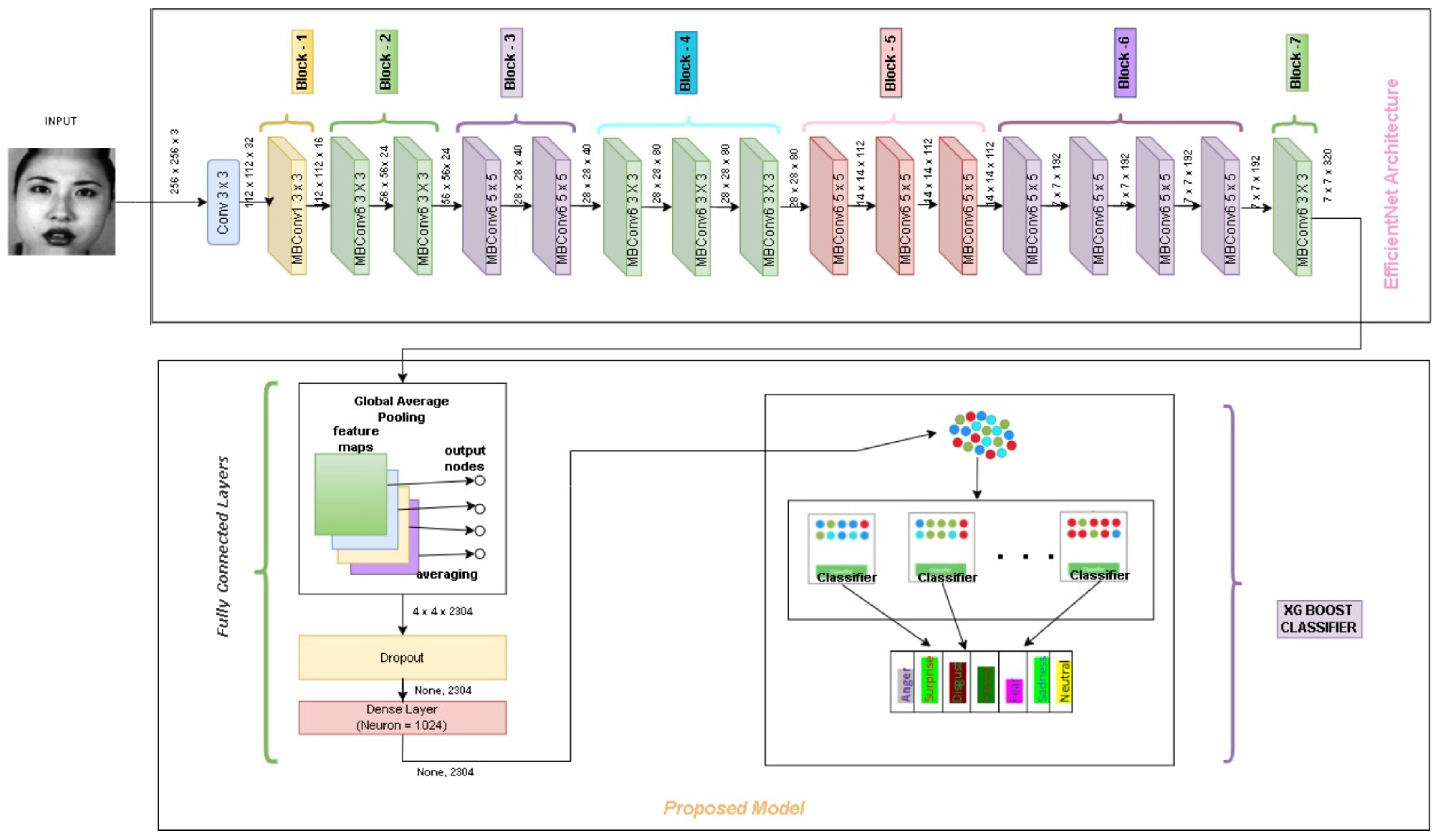
The proposed work consists of 3 modules. First the EfficientNet Module, Fully Connected Layer and Finally the XGBoost Classifier. Figure 3 illustrates the models block diagram. Images are given as input to the EfficientNet and processed for feature extraction.

4.1. Proposed Algorithm

The Algorithm for the EfficientNet-XGBoost is designed in this section. Algorithms 1 and 2 are the step wise refinements of MBConv1 and MBConv6 respectively. Algorithm 3 is the model step wise refinement, MBConv1 and MBConv functions are executed repeatedly as discussed in the model setup Section 3.1.
Algorithm 1: MBConv1(K × K, B, S)
Require: K K e r n e l S i z e , B : O u t p u t F e a t u r e M a p s , S : S t r i d e , R : R e d u c t i o n r a t i o o f S E , T : T o t a l I m a g e s { X 1 , X 2 , . . . X T }
   1: d w c D e p t h w i s e C o n v ( K × K , M , S )
   2: b n B a t c h N o m a l i z a t i o n ( d w c )
   3: s w S w i s h ( b n )
   4: e S E ( R = 4 , s w )
   5: c o n v C o n v ( 1 × 1 , B , 1 , s e )
   6: b n B a t c h N o r m a l i z a t i o n ( c o n v )
   7: return (h/s × w/s, B = bn)
Algorithm 2: MBConv6(K × K, B, S)
Require: Inputs: K : K e r n e l S i z e , B : O u t p u t F e a t u r e M a p s , S : S t r i d e , R: Reduction ratio of SE, T : T o t a l I m a g e s { X 1 , X 2 , X T }
   1: c o n v C o n v ( 1 × 1 , 6 M , 1 )
   2: b n B a t c h N o m a l i z a t i o n ( d w c )
   3: b n B a t c h N o r m a l i z a t i o n ( b n )
   4: s w S w i s h ( b n )
   5: s e S E ( R = 4 , s w )
   6: c o n v C o n v ( 1 × 1 , B , 1 , s e )
   7: b n B a t c h N o r m a l i z a t i o n ( c o n v )
   8: return (h/s × w/s, B = bn)
Algorithm 3: EFFICIENTNET-XGBOOST()
Ensure: weights I m a g e n e t w e i g h t s
Ensure: biases I m a g e n e t B i a s
Ensure: input ( 48 , 48 , 3 ) , T is total images.
  1: begin:
      for i in range(0, T) do
      begin:
      {     conv<-- Conv(3 × 3, image)
          bn <-- BatchNormalization(conv)
          sw <-- bn * sigmoid(bn)}
      end;
  2: m b c 1 M B C o n v 1 ( 3 × 3 , B , S , s w ) 16 rounds
      for i in range(0, 2):
            mbc6 <-- MBConv6(3 × 3, B, S,mbc1)
      for i in range(0, 2):
          mbc6 <-- MBConv6(5 × 5, B, S,mbc6)
      for i in range(0, 3):
          mbc6 <-- MBConv6(3 × 3, B, S,mbc6)
      for i in range(0, 6):
          mbc6 <-- MBConv6(5 × 5, B, S,mbc6)
  3: m b c 6 M B C o n v 6 ( 3 × 3 , B , S ) ( m b c 6 )
  4: c o n v 1 C o n v ( 1 × 1 , M , S ) ( m b c 6 ) Fully Connected Layer
  5: p o o l M a x P o o l 2 D ( pool_size = [1, 1],padding = ’valid’,S = 2)
  6: d D r o p o u t ( 0.5 , p o o l )
  7: d e D e n s e ( N = 1024 , d )
      for i in [feature\_maps]:
        read i:
      begin
        {   train\_y = train[$neurons=1024$]
    train\_x = train.drop[$neurons=1024$]
    dataset = xgboost.Dmatrix(train\_y, train\_x) }
      end:
  8: PARAMS: m a x _ d e p t h = 7 , e t a = 0.2 , n u m c l a s s e s = 7 , o b j e c t i v e = s o f t m a x
  9: X g X G B O O S T . t r a i n ( p a r a m s , d a t a s e t , num_boost_round = 200)
  10: Y h a t X g . p r e d i c t ( x _ t e s t )
  11: s c o r e a c c u r a c y _ s c o r e ( t e s t _ y , Y h a t )
  12: End
  13: O u t p u t : : s c o r e

4.2. Experimental Setup

In our work, we are trying to use the EfficientNet by TL method to extract the features for the given input image, fine tune the model, and finally, classify it using the XGBoost classifier. The model is divided into 3 modules: EfficientNet, Fully Connected Layer, and XGBoost Classifier. First we try to preprocess the images, which is explained in Section 4.4, and then apply TL for feature extraction. EfficientNet is known for obtaining great precision with few parameters and FLOPS (Floating Point Operation Per Second). Traditional CNNs are involved in fine tuning manually. Fine tuning is done in 3 dimensions. There are three of them: the number of layers, the number of channels, and the image size. The compound scaling process is used by EfficientNet for scaling. The Swish function is used, and the following is the mathematical representation:
s w i s h ( x ) = x s i g m o i d ( x )
The image is of size (48 × 48) is given as input. Various phases of feature extraction are performed on the input image by the model. The model architecture consists of seven inverted residual blocks denoted by MBConv and two residual blocks denoted by Conv. In Table 1, detailed information about each layer of the EfficientNet-B0 baseline network is shown. Both MBConv1, k3 × 3, and MBConv6, k3 × 3, employ depthwise convolution, which combines the 3 × 3 kernel size with s as the stride size. Both of these blocks comprise batch normalization, activation, and convolution. They have a kernel size of 1 × 1. The classifier and expression predictor is XGBoost. XGBoost is replaced with softmax, for best performance and accuracy.
Model Training and Evaluation: The model execution for training and testing was performed on Google Colab Cloud Platform. Tensorflow 2.6 was used on Python 3.7, and the GPU was a Tesla P100-PCIE-16GB. The CPU is an Intel(R) Xeon(R) CPU running at 2.20 GHz. The researchers can reuse the weights learned and unfreeze some layers as per requirement to perform training, thanks to TL, helped for developing FER system. We have used Adam optimizer an adaptive learning rate method for training. The batch size considered is 32 with epochs ranging from 100–150. The parameters used are shown in Table 2.

4.3. Datasets

To measure the performance of the proposed model, we have chosen 4 datasets for facial emotion. Table 3 shows the no of sample images in each category of different datasets.

4.3.1. CK+

The (CK+) [28] was published in the year 2010. CK+ is an extension of the Cohn-Kanada dataset is used in our research which contains 7 types of basic expressions. The images of this dataset are in size of 48 × 48. They are Anger, Disgust, Fear, Happiness, Sadness, Surprise with sample size of 135, 177, 75, 207, 84, 249 respectively. This makes it a total count to be 927 images. The dataset split for Training is 648, Validation is 139 and Testing is 140 images.

4.3.2. KDEF

In total, the Karolinska Directed Emotional Faces (KDEF) dataset [31] contains 490 images of human facial expressions. The images in this dataset are 256 × 256 in size. This dataset contains 7 emotion classes as mentioned similar to Section 4.3.1. Here the samples are distributed evenly, with 70 images of each type.

4.3.3. JAFFE

The JAFFE [26] dataset consists of 180 images of 6 basic classes. The images in this dataset are of size 120 × 120. The emotion classes are Sad, Disgust, Fear, Surprise, Anger and Happy with 30 images each.

4.3.4. FER2013

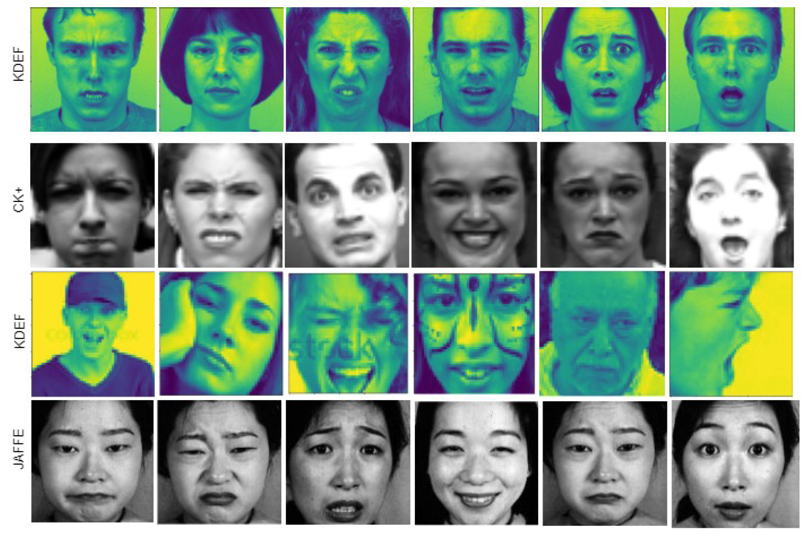
The FER2013 [28], very challenging dataset consists of 35,887 face image samples. 28,709 images for training and 3589 images for training and testing each. The images in this dataset are set to grayscale. The images are of size 48 × 48. The samples are categorized into 7 classes of emotions. 0—Anger, 1—Disgust, 2—Fear, 3—Happy, 4—Sad, 5—Surprised and 6—Neutral. We discovered some label errors in the test dataset during the experiment. This dataset’s benchmark accuracy is only (65 + 5) percent, which is extremely difficult. Even so, most researchers continue to use this dataset to test their models. A snapshot of the samples is presented in Figure 4.

4.4. Data Pre-Processing

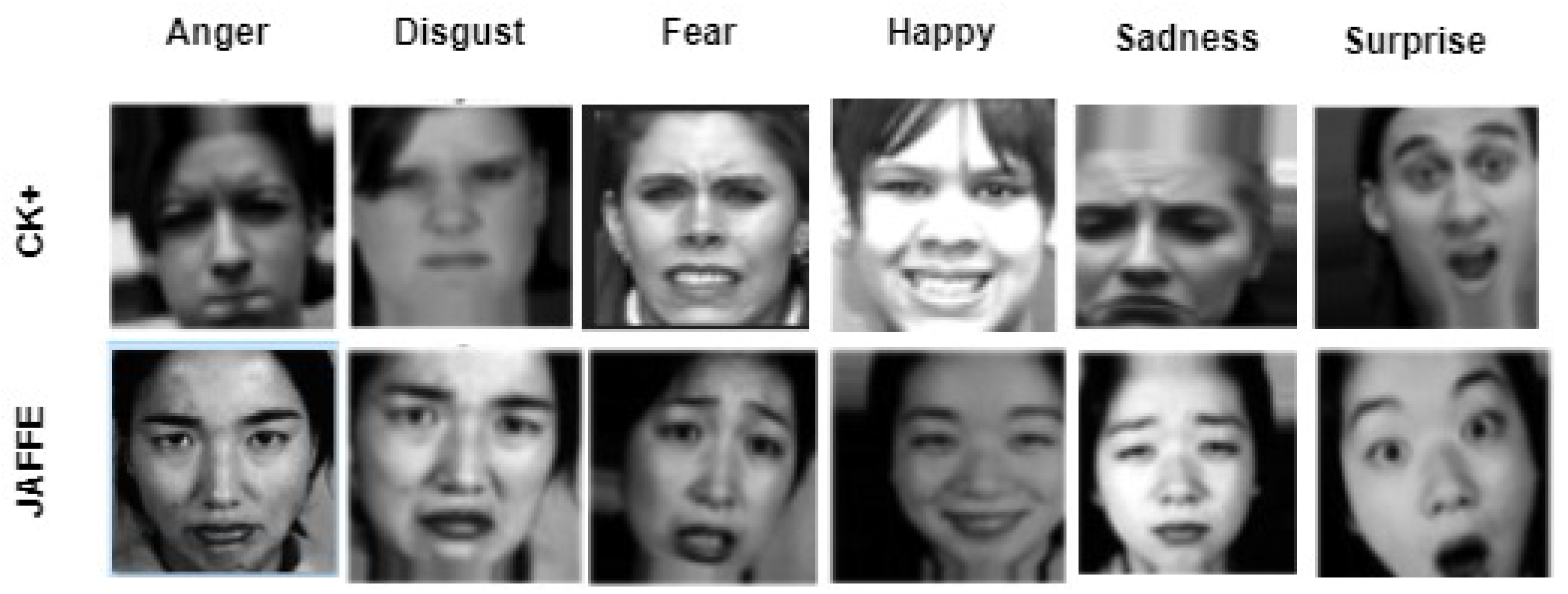
It is very natural that we need to process the image before training. Data sets namely KDEF and FER2013 are in Comma Separated Values .CSV format. CK+ dataset and JAFFE are in .jpg images. During the preprocessing phase, we reshaped the images into an acceptable format for the model. If we look at Table 3 for the FER2013 and CK+ datasets, we can see that all of the images in classes are not equal. Few classes have a larger sample size, while others have fewer samples. This is referred to as class-imbalance. To overcome this type of issue, we must include additional images into the classes with fewer samples. This is possible with the help of data-augmentation. Augmentation aids in increasing the size of the data set as Table 4. The more variation in the train data, the better the model learns. In this work, data is augmented is carried out artificially through geometric transformation techniques like translation, reflection, shearing, and other means [20]. The augmented image samples generated during the pre-processing phase are shown in Figure 5.
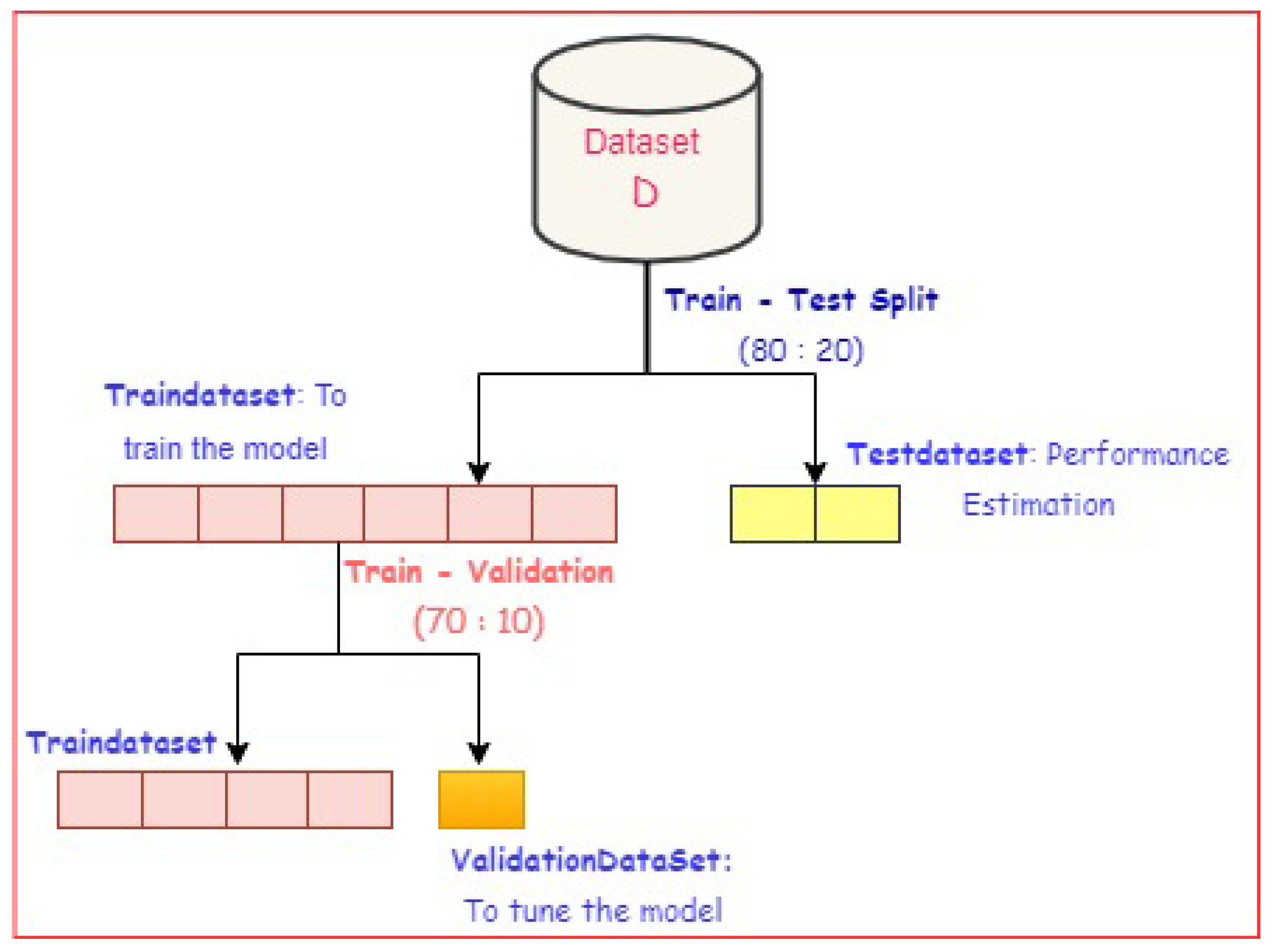
The dataset has three sections: train data, validate data, and test data. In our model, we used an 80/20 split to train the model and the remaining 20% to test the model’s performance. To avoid performance errors, 10% of train data is split into validation data using parameter adjustment. After the model has been trained, test data is used to assess the model’s performance. Figure 6 clearly represents splitting of data into Train, Test and Validation.
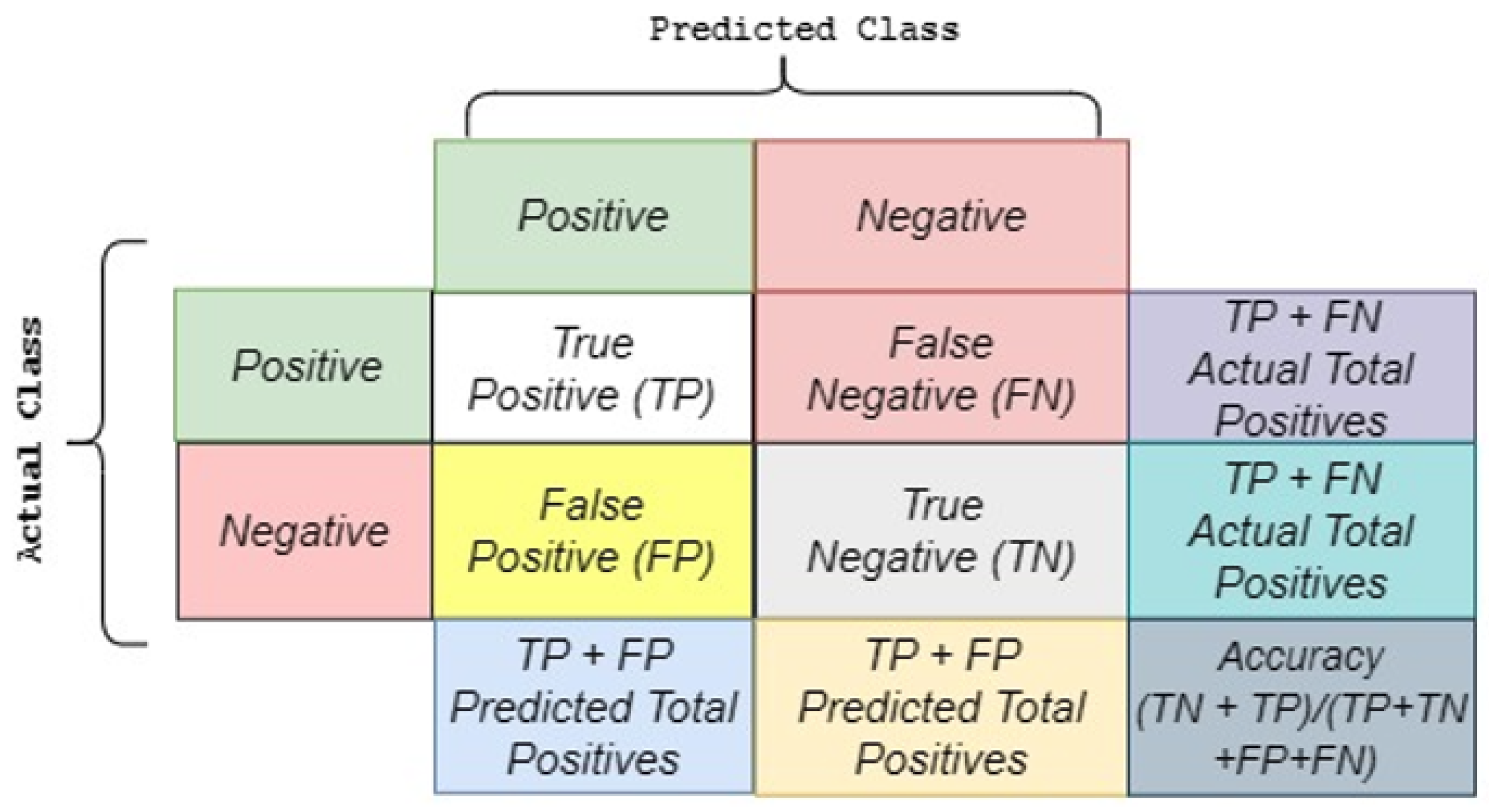
A confusion matrix is used to evaluate a classification’s performance. The confusion matrix (as shown in Figure 7) is calculated for finding the class’s accuracy. It’s represented as a matrix. The confusion matrix allows for a comparison of actual and predicted values. The confusion matrix for N-class classification is N × N. True Positive ( T P ) , False Positive ( F P ) , True Negative ( T N ) , and False Negative ( F N ) are the four terms that make up the confusion matrix ( F N ) . Representation of confusion matrix is shown in Figure 7.
Accuracy: Accuracy is calculated by dividing the total number of predicted values by the total number of predictions made by the model. The formula below represents accuracy.
A c c u r a c y = TP + TN TP + FN + FP + TN
Accuracy gives a false sense of prediction if the dataset is imbalanced.
Precision: Precision is the percentage of true positive predictions out of all positive predictions. Precision is denoted by the following equation:
P r e c i s i o n = TP TP + FP
Recall: What proportion of the total positive is predicted to be positive? It’s the same as TPR (True Positive Rate). The formula is represented as:
R e c a l l = TP TP + FN
F1-score: The harmonic mean of precision and recall is defined. It’s a statistical metric for evaluating performance.
F 1 S c o r e = 2 R e c a l l P r e c i s i o n R e c a l l + P r e c i s i o n
ROC AUC: Receiver Operating Characteristics (ROC) is a graph that compares the true positive rate (on the y-axis) and false positive rate (on the x-axis) for every classification threshold that is conceivable. ROC-AUC stands for the area determined under the ROC curve.
R O C A U C = 1 + T P F P 2
It represents the probability that a model ranks randomly positive observation higher than the randomly chosen negative observation, and thus it is a useful metric. We can see parameters used for XGBoost as Table 5.

5. Results and Discussion

In this section, confusion matrix analysis, classification performance analysis, accuracy, and feature maps of the proposed model EfficientNet-XGBoost are discussed clearly.

5.1. Training and Validation

The model is trained and validated with the training dataset. Loss must be reduced in order to fine-tune the model. The accuracy and loss corresponding to validation process are represented through a plot respectively in Figure 8. In Figure 8a, the plot related to training and validation accuracy is shown. The X-axis represents the count of epochs and the Y-axis represents the rate of accuracy, scaled from 0.3 to 1.0, where 0.3 is 30% and 1.0 is 100% accuracy, and Figure 8b is the plot for training and validation loss. The linear axis represents the count of epochs, and the vertical axis represents the measure of loss. These plots represent the model training and validation on the CK+ dataset. From Figure 8a, it is clearly observed that 100% accuracy is obtained on training and validation of the dataset. The accuracy measure corresponding to test samples is presented in the results section in the form of a confusion matrix.

5.2. Analysis Using Confusion Matrix

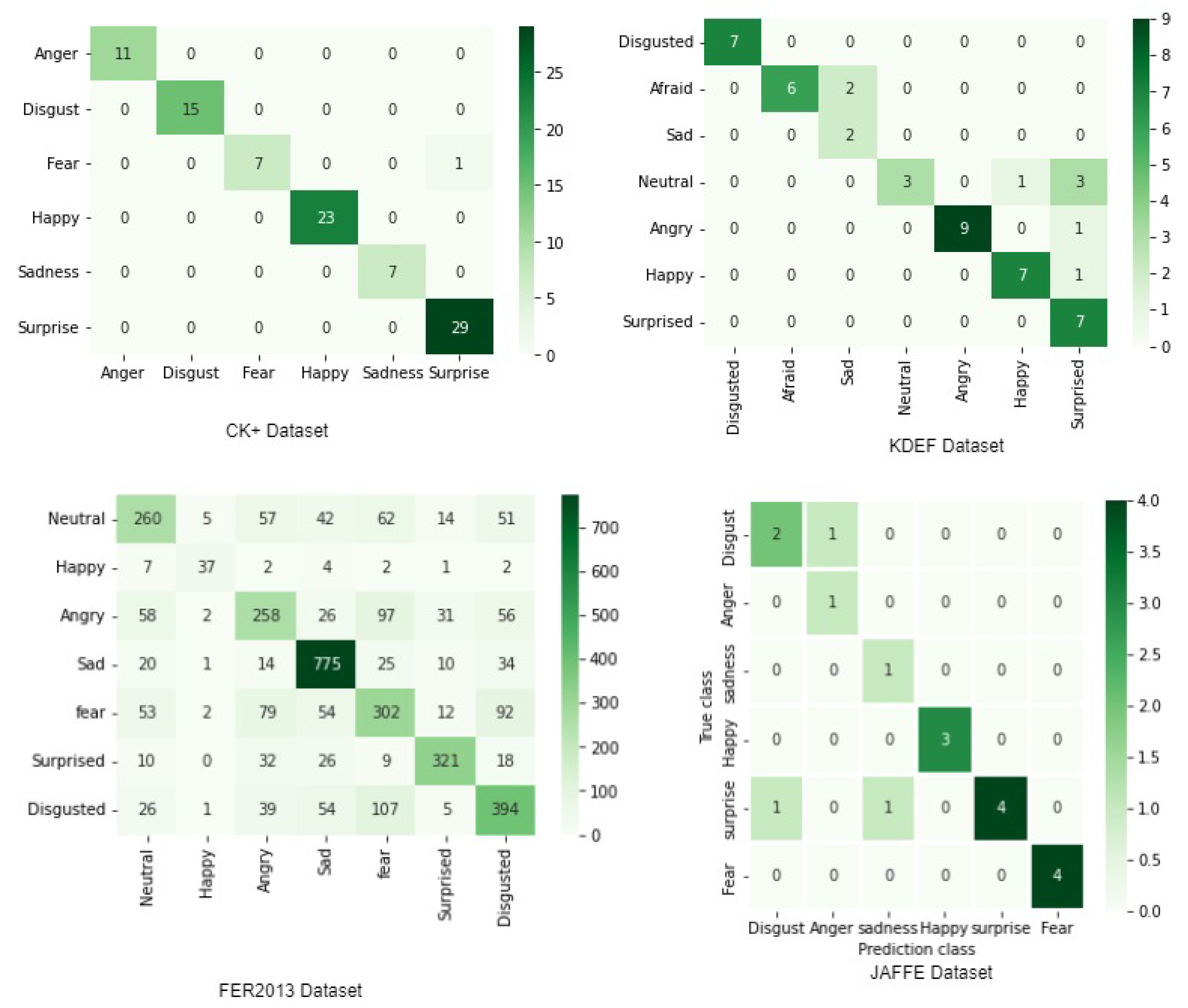
The confusion matrix is primarily utilized for comparing the classifier outcomes with the actual class level. This helps in genuine evaluation of the classifier model. The confusion matrices in Figure 9 are derived from the datasets CK+, KDEF, FER2013, and JAFFE. As shown in Figure 9, each class’s prediction accuracy is concentrated along the diagonal. Each of the confusion matrices has the predicted class and the true class. In contrast to Fer2013’s data set, which has low classification accuracy, the CK+ data set’s seven categories have high prediction accuracy. Fer2013 is a very large and challenging dataset which has class imbalance. Despite this, the most popular data set for facial expression recognition is Fer2013. The experiment also uses the Fer2013 dataset to compare outcomes with other approaches using the same parameters. If we look at the CK+ dataset, all the emotions are correctly identified, except that the emotion “fear” is classified as “surprise”. Figure 9 also depicts the confusion matrix of the KDEF and JAFFE data sets. We can see from the confusion matrix results that the proposed method has good classification performance.
For the KDEF dataset also, if we observe the figure, 8 images are misclassified. 4 images of neutral emotions are classified as 1 happy and 3 surprise emotions. One image of a happy emotion and one image of anger are misclassified as surprise. There are clearly a lot of misclassified emotions in FER2013 dataset. This is due to the large size and very challenging dataset. For the JAFFE dataset, we have 4 misclassified emotions. One disgust image is identified as an angry image, one surprise image is identified as a disgust image, and finally, one surprise image is identified as sadness. This is due to the similarity expression in the dataset. Also, to train the model, we have a very small number of images per class.

5.3. Analysis of Classification Performance

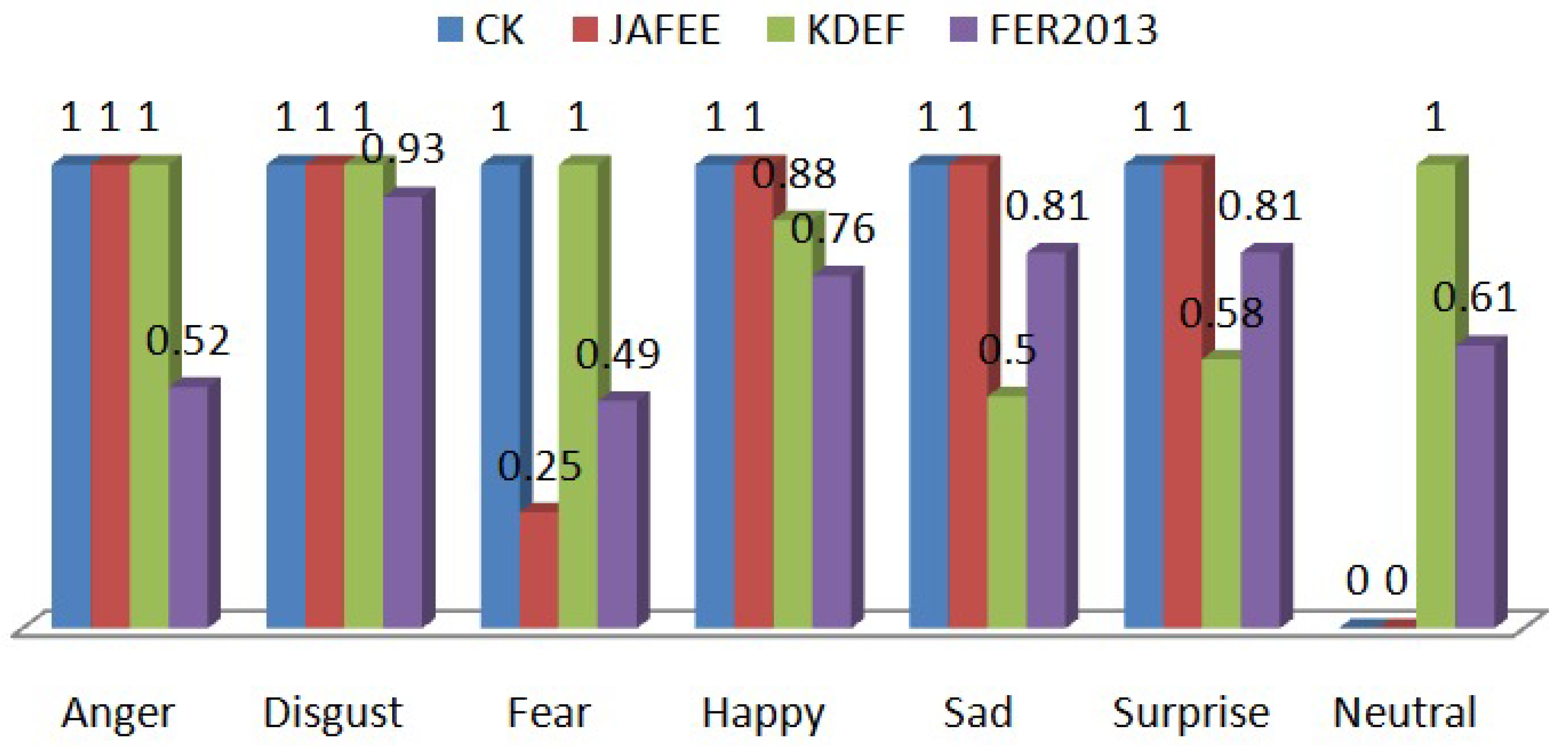
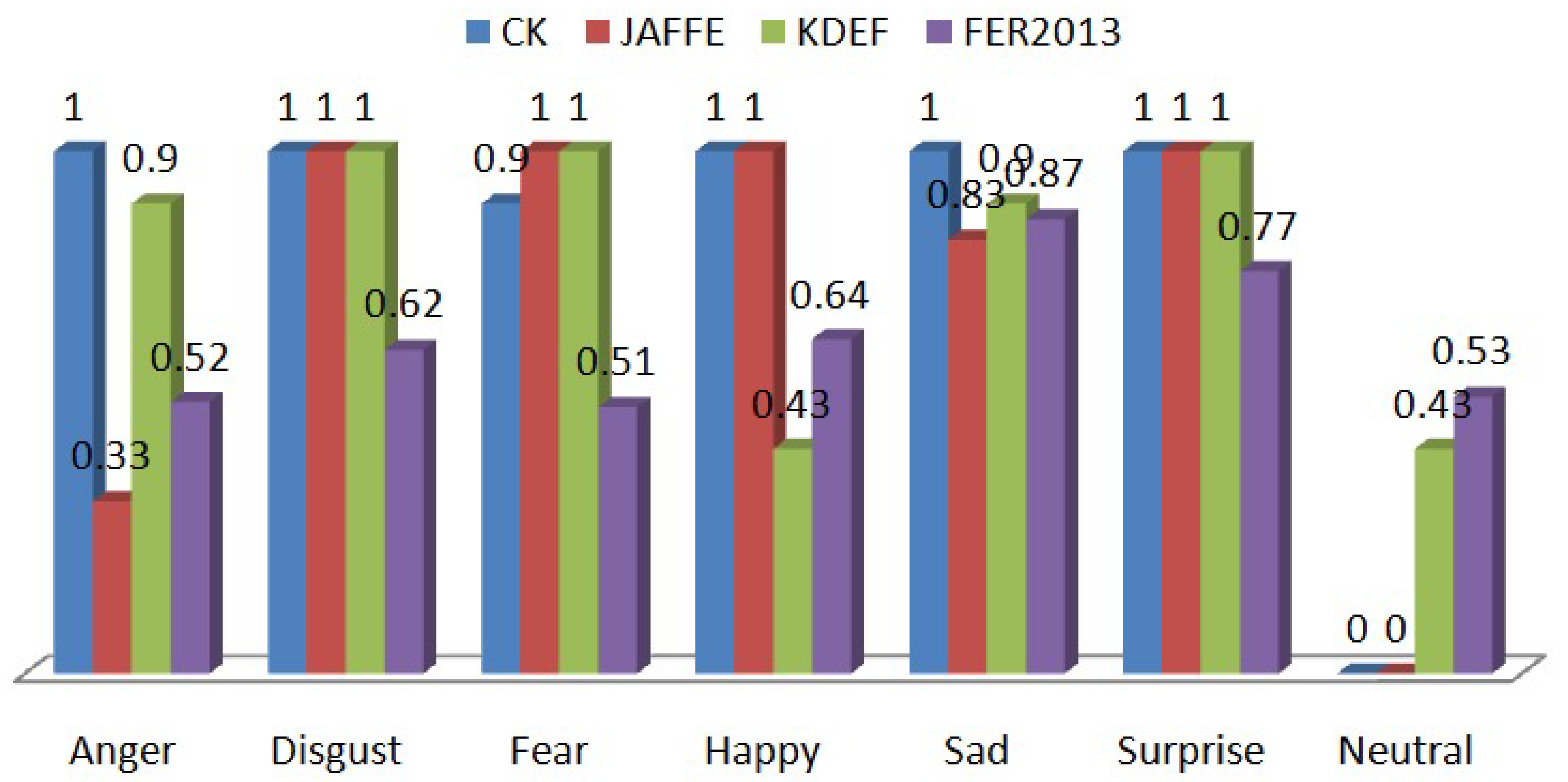
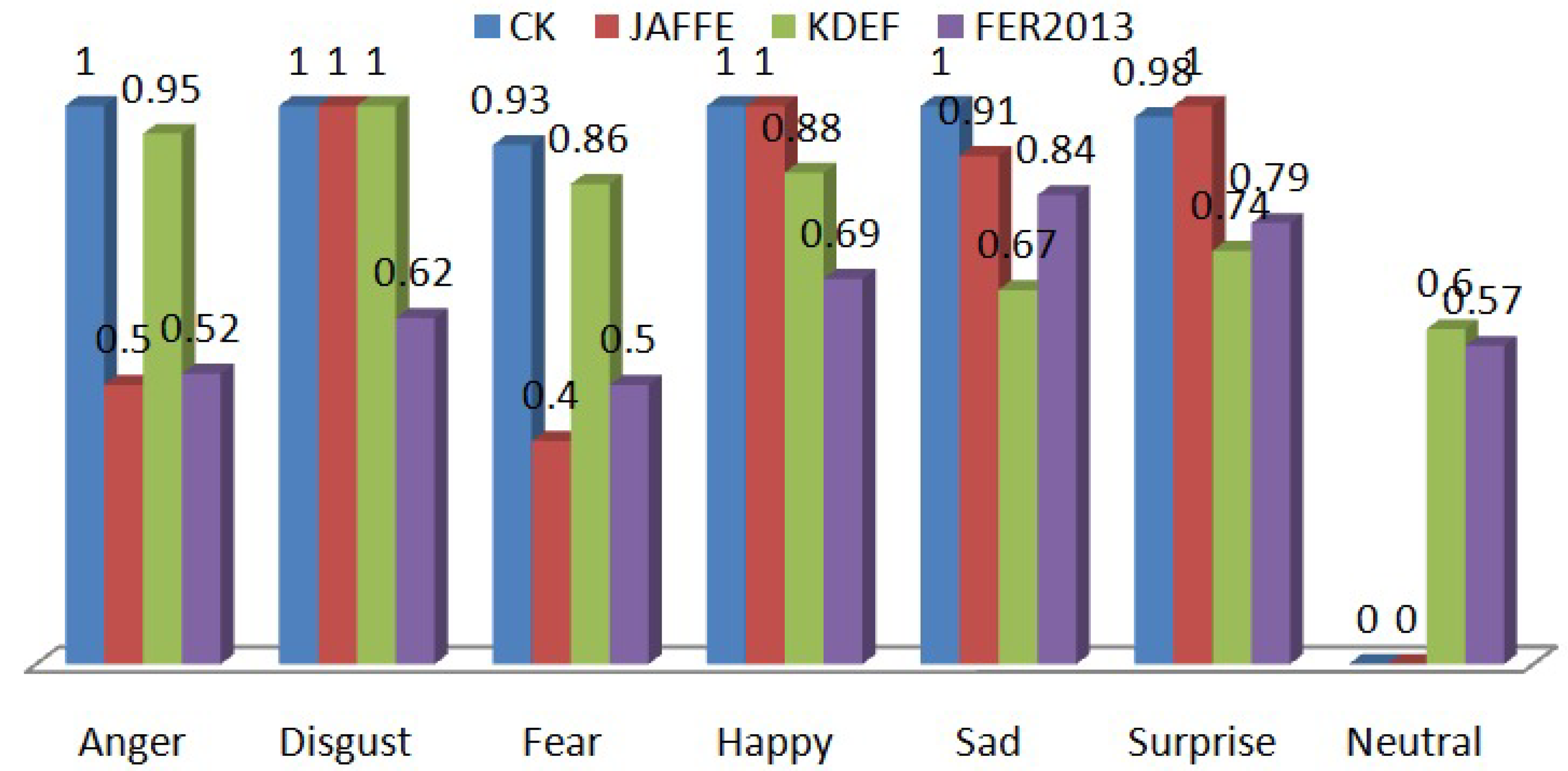
Figure 10, Figure 11, Figure 12 and Figure 13 shows the Precision, Recall, F1-Score, and Support of the proposed model EfficientNet-XGBoost on the CK+, KDEF, JAFFE, and FER2013 datasets. It is clearly observed that from Figure 10, Figure 11 and Figure 12 all the evaluation shown for each emotion classes of CK+ dataset is very high. The FER2013 dataset is low. The reason for this is due to FER2013 dataset is very challenging dataset. These figures represent the classification performance of the model. The representation is in the form of bar plots. In the figures, X-Axis represents classes of emotions of 4 datasets. The CK+ and JAFFE datasets have six categories of emotions. The FER2013 and KDEF datasets each contain seven categories of emotions. Y-Axis represents the percentage of accuracy, scaling from 0.00 to 1.00 range. The order of the datasets represented in the plot is CK+, JAFFE, KDEF, and FER2013.
Precision is shown in Figure 10. The bar plot show emotions on the X-Axis. It is very clear that for Anger, Disgust, Fear, Happy, Sad and Surprise shows 1, which indicates that these emotions achieved 100% precision measure for CK+, JAFFE and KDEF dataset. For the datasets CK+ and JAFFE the expression NEUTRAL is not available. Hence marked as zero.
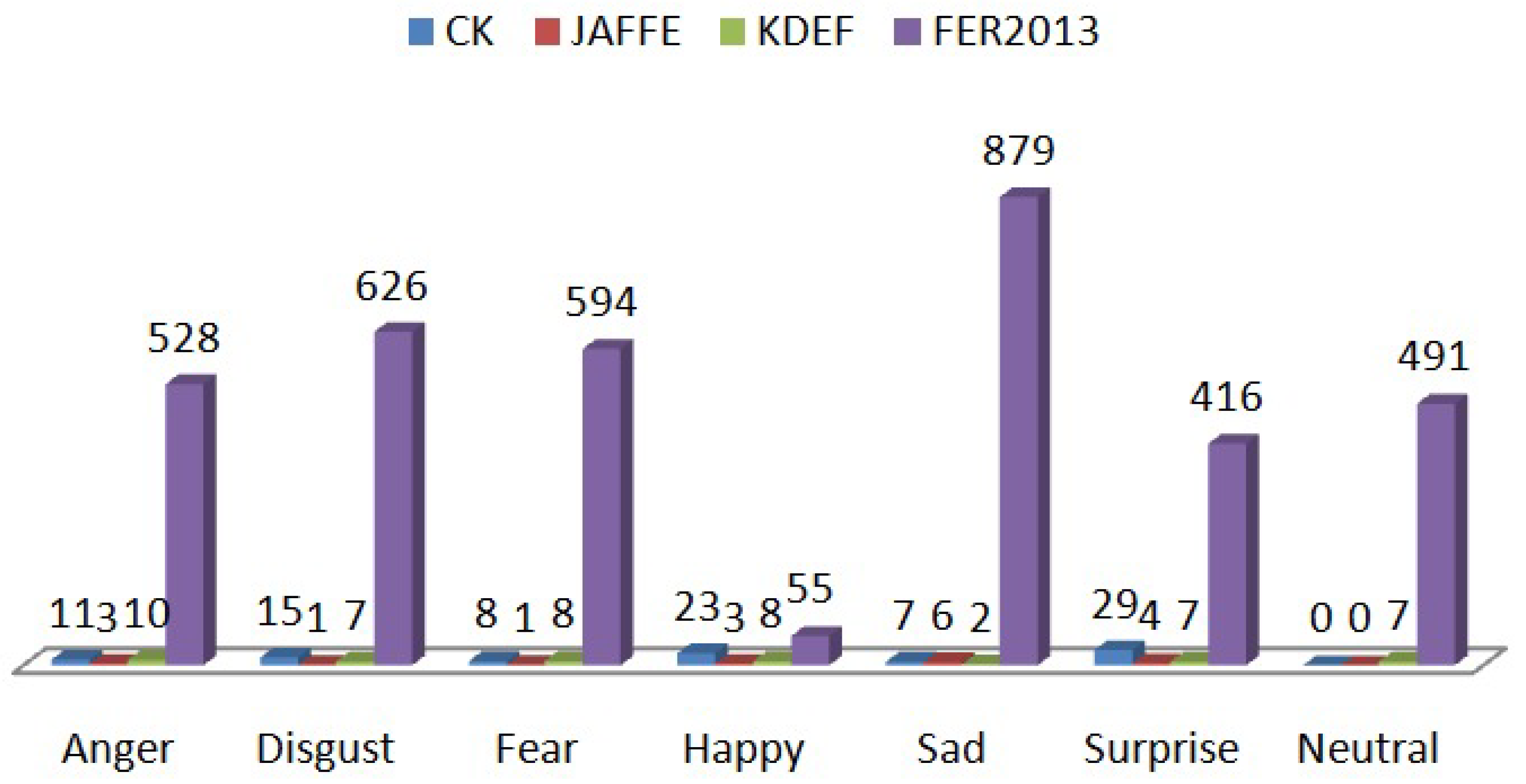
Recall is shown in Figure 11, anger, fear, happy, sad and surprise emotions for CK+, JAFFE and KDEF achieved 100%. Fear emotion is 90%. for CK+ dataset, this is due to class imbalance. It has only 75 sample in the dataset. A very less sample for the model to train. Recall in Anger class of JAFFE dataset is 33%. The reason behind this is the images are very similar to fear emotion. This is the challenge in this dataset. The F1-Score for the model is calculated. It is shown in Figure 12. From figure, we can see that the best results for CK+ and KDEF datasets are very close to 100% for anger, disgust, fear, happiness, sadness, and surprise. Support for the datasets CK+, JAFFE, KDEF, and FER2013 is shown in Figure 13. The number of samples of the true prediction that fall into each class of target values can be used to determine support. The structural weakness in the scores represents the imbalanace state of the training data. Low value of support, leads either for stratified sampling or rebalancing.

5.4. Feature Maps

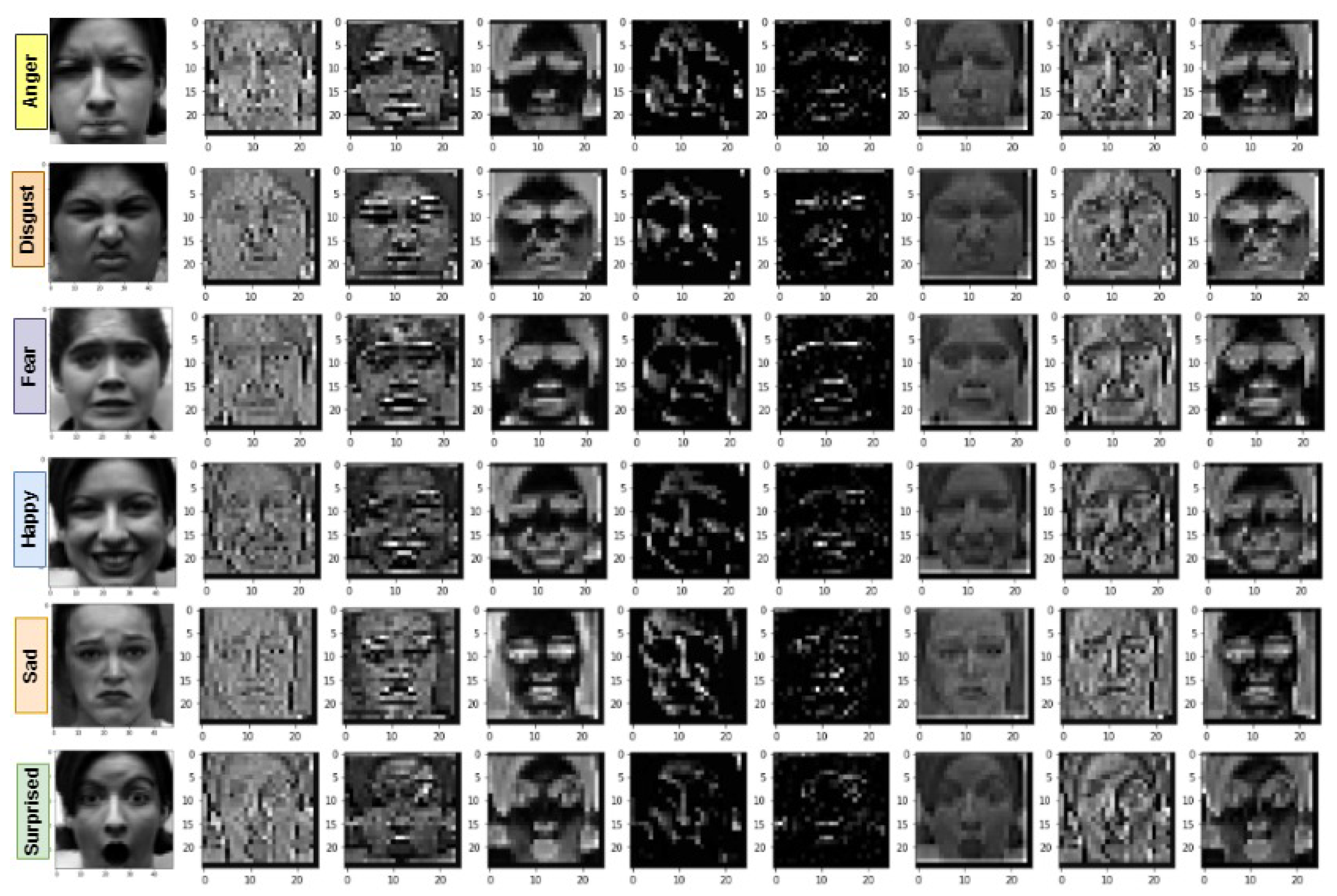
Verification of the feature extraction can be done by visualising the feature sets for the images in different layers. The major objective to visualize a feature set corresponding to particular input image is to gain some understanding about the inherent characteristics. The proposed model thus, gains further insights of the inputs. Perhaps it detects some parts that we desire to extract. It is very interesting to directly examine the features like colors and edges, which are known as low-level features, and high level features like shapes and objects. In our model, it’s easy to see that the eyes, nose, and lips are all there.
Feature maps for the images at random layers are shown in Figure 14. In Figure 14 we see that the features extracted by each layer from the face’s most significant features.

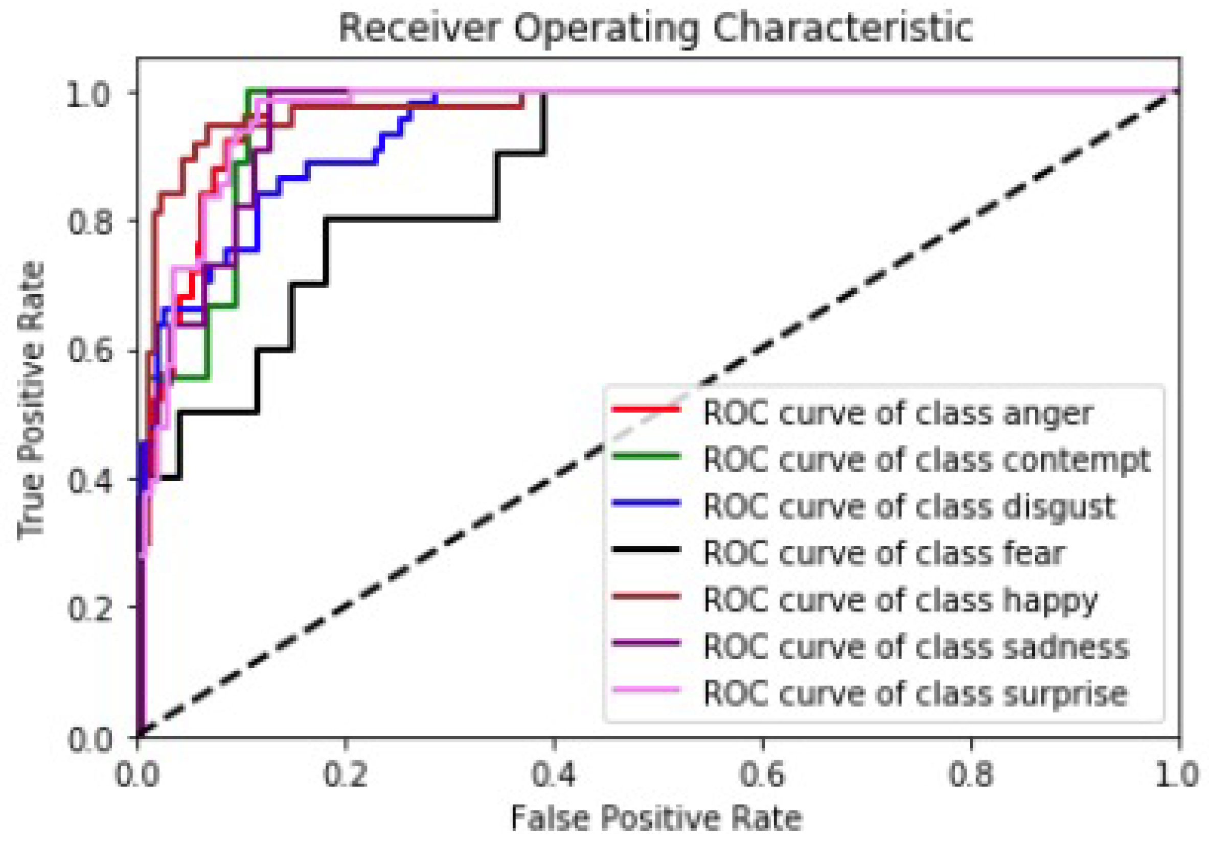
5.5. Receiver Operating Characteristic

The area under the curve (AUC) values and receiver operating characteristic (ROC) curves were computed in order to further assess the results of each expression’s recognition. It is a curve of probability that plots the True Positive Rate (TPR) over False Positive Rate (FPR) at different threshold values and essentially separates the signal from the noise. The ROC for the CK+ dataset is shown in Figure 15. X_axis represents the false positive rate and Y_axis represents the true positive rate. The colored curves indicate different classes. As shown in Figure 15 black curve which is far away from other curves and at the bottom represents fear emotion. Fear emotion is falsely predicted as a surprise (Figure 9) emotion of the cK+ dataset. The accuracy of the Fear class is less when compared with other emotions.

5.6. Comparison of Results with Other Works

This section presents an investigation on the efficacy of the stated model on benchmark datasets. EfficientNet-XGBoost, the developed model, is entirely based on the transfer learning technique. Because EfficientNet is the foundation of the proposed model, it is thoroughly tested to determine how well it works. Table 6 represents the results for the accuracy in training, validation, and test images experimented with the base model EfficientNet. The dataset was split into 80% and 20% for training and testing data. We have experienced that feature extraction was done efficiently by this model. Here, the softmax layer helps in classifying emotions. We replace this softmax layer with the machine learning algorithm XGBoost to improve accuracy. The proposed EfficientNet-XGBoost method can efficiently extract image features and enhance the accuracy of facial expression recognition.
Suitable simulations are carried out on the same train/test split using notable methods from the literature. To fully validate the proposed method’s effectiveness, for comparison under the same conditions, 20 related expression recognition techniques are chosen. Table 7, Table 8, Table 9 and Table 10 shows the accuracy of other models compared with our model EfficientNet-XGBoost on CK+, JAFFE, KDEF and FER2013 datasets respectively.
A weighted mixture deep neural network (WMDNN) [32] was proposed and tested on the CK+ dataset with 97.02% accuracy. SIFT-CNN, a hybrid model proposed by X. Sun and M. Lv [33], has a 94.82 percent accuracy. In [23] AdaBoost was used to segment the face’s largest geometric component, and multistage Haar wavelet was used to extract the features of the components. AdaBoost, on the other hand, is sensitive to abnormal samples, which will result in higher weights in the iterative process and thus affect segmentation performance. In the meantime, using the Haar wavelet base will result in inefficient feature extraction. The recognition accuracy of this model for the CK+ data sets is 90.48 percent. This model has a very low recognition accuracy when compared to other methods. A region-aware sub-net (RASnet) [34] learns binary masks for locating expression-related critical regions with coarse-to-fine granularity levels, whereas an expression recognition sub-net (ERSnet) with a multiple attention (MA) block learns comprehensive discriminate features. This model achieved 96.28% accuracy.
Among the models [33,34] in the above comparison, two have used traditional methods for mining expression recognition. Shi, Cuiping, et al. [25] created a CNN model based on a residual network. Before extracting the features from the expression images, this model first preprocesses the input images. The accuracy of feature extraction is increased to 98.48 percent after being extracted by various network branches and then fused together, which is higher than other methods but lower than our accuracy.
From Table 7 our model EfficientNet-XGBoost has achieved 100% accuracy when compared with other models. This was achieved with epoch of 150 on dataset CK+.
Table 8 shows the accuracies of the KDEF dataset with other models. [28] identifies the features through the Facial Landmarks descriptor and the Center of Gravity descriptor. On KDEF, these features are classified by Support Vector Machine (SVM) with an accuracy of 90.80% which is the lowest accuracy among the comparisons. The stacked Convolutional Auto-Encoder (SCAE) [28] model is proposed and used random weights for training the images. Random weights will take many person-hours. Convolution layers and a recurrent neural network (RNN) are the two components of the network architecture that Jain et al. [31] proposed. The combined model extracts relationships within facial images, and by using the recurrent network, the temporal dependencies that exist in the images can be taken into account during classification.
The accuracy of our model using the JAFFE dataset is compared with other works in Table 9. For the FER task, [26] proposes a model called the Vision Transformer in conjunction with a Squeeze and Excitation (SE) block. with an accuracy of 94.83% which is a bit low compared to our work. Vision transformers require large datasets, whereas JAFFE only has a small number of samples. image distribution of JAFFE is shown in Table 3. The JAFFE dataset has only 180 images, but they are equally distributed with all 7 classes of emotions. The paper [2] proposes a deep learning strategy based on an attentional convolutional network, which is capable of focusing on key facial features such as the nose, eyes, lips, and cheeks. The accuracy of [14] is 92.8%. The proposed models’ accuracy using the JAFFE dataset would be high if the number of samples were greater. This attention was drawn during experimentation.
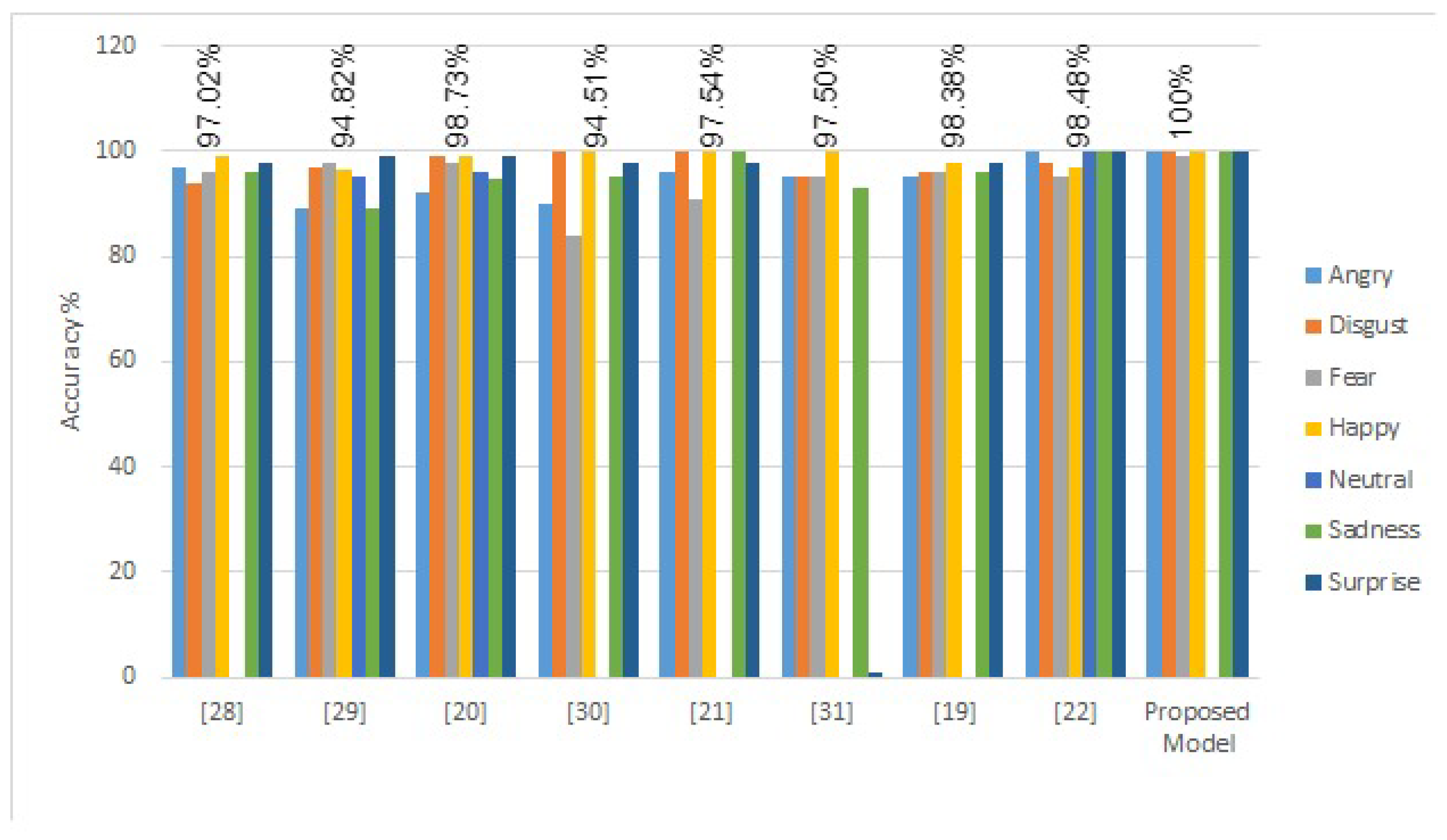
The model’s test results for each class are compared to other works. The overall accuracy of the model is directly proportional to the accuracy of the individual classes. Figure 16 shows the accuracy achieved by our model and others on individual classes of emotions. X_axis denotes the works and Y_axis denotes accuracy. It is observed from Figure 16 that our proposed work achieves 100% accuracy for each emotion class except Fear. Six basic facial emotion classes are depicted in the figure. Though, some researchers have also included Neutral as one of the emotions. The proposed model, EfficientNet-XGBoost, has shown the best performance on the CK+ dataset. The JAFFE dataset and KDEF dataset contain frontal images. The FER2013 dataset is a challenging dataset with 35,887 sample images, which did not produce high accuracy but was equal to the benchmark accuracy. The major issue with this dataset is the class imbalance. Proper augmentation needs to be done by producing synthetic images rather than augmenting them using geographic features.

6. Conclusions and Future Scope

An efficient scheme with a state-of-the-art transfer learning mechanism has been presented suitably for facial emotion recognition. The scheme is dubbed as EfficientNet-XGBoost. Novelty of the scheme is exhibited with certain combination of pre-trained EfficientNet architecture, fully connected layers, XGBoost classifier, and custom fine-tuning of parameters. Input facial images are suitably pre-processed and the task of feature extraction is carried out through using the custom model. The feature points are extracted through various networks. To average the feature maps, the global average pooling is applied and the final feature set is fed to XGBoost Classifier which recognizes the class labels for distinct emotions. Four distinct datasets are used to validate the scheme. The experimental results for the dataset CK+ shows outstanding performance at an overall rate of accuracy of 100%. Further, the proposed model can recognize expressions accurately with low latency. An overall rate of accuracy of 98% is observed on datasets like JAFFE and KDEF. In FER2013, although the sample distribution is imbalanced, augmentation through geometric transformation techniques has led to reach a benchmark accuracy of 72.54%. In support of our claim, a comparative analysis of our results with other works on existing datasets is presented. The future scope of the work would be to mitigate the issue of increasing its efficiency for imbalanced sample sets. Exploring the use of custom GAN (generative adversarial networks) could be a wise consideration towards the recognition of facial expressions from the imbalanced datasets.

Author Contributions

Conceptualization, S.B.P., S.K.K., T.K.M., H.M. and S.R.M.; Methodology, S.B.P., T.K.M., A.A. and H.M.; Software, S.B.P., S.K.K., T.K.M., A.A., H.M. and S.R.M.; Validation, S.B.P., S.K.K., T.K.M., A.A. and H.M.; Formal analysis, S.B.P., S.K.K., T.K.M. and A.A.; Investigation, S.B.P., S.K.K. and T.K.M.; Resources, S.B.P., S.K.K. and H.M.; Data curation, S.B.P., T.K.M., H.M. and S.R.M.; Writing—original draft, S.B.P., S.K.K., T.K.M., A.A., H.M. and S.R.M.; Writing—review and editing, S.B.P., S.K.K., T.K.M., H.M. and S.R.M.; Visualization, S.B.P., S.K.K. and H.M.; Supervision, S.B.P., S.K.K., M.K. and H.M.; Project administration, S.B.P., S.K.K., M.K. and H.M.; Funding acquisition, M.K. All authors have read and agreed to the published version of the manuscript.

Funding

This research received no external funding.

Data Availability Statement

Not applicable.

Conflicts of Interest

The authors declare no conflict of interest. No financial support has been received from any agency for the proposed work.

References

  1. Akhand, M.; Roy, S.; Siddique, N.; Kamal, M.A.S.; Shimamura, T. Facial emotion recognition using transfer learning in the deep CNN. Electronics 2021, 10, 1036. [Google Scholar] [CrossRef]
  2. Minaee, S.; Minaei, M.; Abdolrashidi, A. Deep-emotion: Facial expression recognition using attentional convolutional network. Sensors 2021, 21, 3046. [Google Scholar] [CrossRef] [PubMed]
  3. Goodfellow, I.J.; Erhan, D.; Carrier, P.L.; Courville, A.; Mirza, M.; Hamner, B.; Cukierski, W.; Tang, Y.; Thaler, D.; Lee, D.H.; et al. Challenges in representation learning: A report on three machine learning contests. In Proceedings of the International Conference on Neural Information Processing, Daegu, Republic of Korea, 3–7 November 2013; Springer: Berlin/Heidelberg, Germany, 2013; pp. 117–124. [Google Scholar]
  4. Pons, G.; Masip, D. Supervised committee of convolutional neural networks in automated facial expression analysis. IEEE Trans. Affect. Comput. 2017, 9, 343–350. [Google Scholar] [CrossRef]
  5. Wen, G.; Hou, Z.; Li, H.; Li, D.; Jiang, L.; Xun, E. Ensemble of deep neural networks with probability-based fusion for facial expression recognition. Cogn. Comput. 2017, 9, 597–610. [Google Scholar] [CrossRef]
  6. Jabid, T.; Kabir, M.H.; Chae, O. Robust facial expression recognition based on local directional pattern. ETRI J. 2010, 32, 784–794. [Google Scholar] [CrossRef]
  7. Mahendran, A.; Vedaldi, A. Visualizing deep convolutional neural networks using natural pre-images. Int. J. Comput. Vis. 2016, 120, 233–255. [Google Scholar] [CrossRef]
  8. Wang, K.; Peng, X.; Yang, J.; Meng, D.; Qiao, Y. Region attention networks for pose and occlusion robust facial expression recognition. IEEE Trans. Image Process. 2020, 29, 4057–4069. [Google Scholar] [CrossRef]
  9. Simonyan, K.; Vedaldi, A.; Zisserman, A. Learning local feature descriptors using convex optimisation. IEEE Trans. Pattern Anal. Mach. Intell. 2014, 36, 1573–1585. [Google Scholar] [CrossRef]
  10. Tan, M.; Le, Q. Efficientnet: Rethinking model scaling for convolutional neural networks. In Proceedings of the International Conference on Machine Learning, PMLR, Long Beach, CA, USA, 9–15 June 2019; pp. 6105–6114. [Google Scholar]
  11. Yao, T.; Qu, C.; Liu, Q.; Deng, R.; Tian, Y.; Xu, J.; Jha, A.; Bao, S.; Zhao, M.; Fogo, A.B.; et al. Compound figure separation of biomedical images with side loss. In Deep Generative Models, and Data Augmentation, Labelling, and Imperfections; Springer: Berlin/Heidelberg, Germany, 2021; pp. 173–183. [Google Scholar]
  12. Zhao, M.; Jha, A.; Liu, Q.; Millis, B.A.; Mahadevan-Jansen, A.; Lu, L.; Landman, B.A.; Tyska, M.J.; Huo, Y. Faster Mean-shift: GPU-accelerated clustering for cosine embedding-based cell segmentation and tracking. Med. Image Anal. 2021, 71, 102048. [Google Scholar] [CrossRef]
  13. Jin, B.; Cruz, L.; Gonçalves, N. Pseudo RGB-D Face Recognition. IEEE Sens. J. 2022, 22, 21780–21794. [Google Scholar] [CrossRef]
  14. Yosinski, J.; Clune, J.; Bengio, Y.; Lipson, H. How transferable are features in deep neural networks? Adv. Neural Inf. Process. Syst. 2014, 27, 3320–3328. [Google Scholar]
  15. Chen, T.; Guestrin, C. Xgboost: A scalable tree boosting system. In Proceedings of the 22nd ACM Sigkdd International Conference on Knowledge Discovery and Data Mining, San Francisco, CA, USA, 13–17 August 2016; pp. 785–794. [Google Scholar]
  16. Feng, X.; Pietikäinen, M.; Hadid, A. Facial expression recognition based on local binary patterns. Pattern Recognit. Image Anal. 2007, 17, 592–598. [Google Scholar] [CrossRef]
  17. Liew, C.F.; Yairi, T. Facial expression recognition and analysis: A comparison study of feature descriptors. IPSJ Trans. Comput. Vis. Appl. 2015, 7, 104–120. [Google Scholar] [CrossRef]
  18. Zhao, X.; Shi, X.; Zhang, S. Facial expression recognition via deep learning. IETE Tech. Rev. 2015, 32, 347–355. [Google Scholar] [CrossRef]
  19. Mollahosseini, A.; Chan, D.; Mahoor, M.H. Going deeper in facial expression recognition using deep neural networks. In Proceedings of the 2016 IEEE Winter Conference on Applications of Computer Vision (WACV), Lake Placid, NY, USA, 7–10 March 2016; IEEE: Piscataway, NJ, USA, 2016; pp. 1–10. [Google Scholar]
  20. Shima, Y.; Omori, Y. Image augmentation for classifying facial expression images by using deep neural network pre-trained with object image database. In Proceedings of the 3rd International Conference on Robotics, Control and Automation, Chengdu, China, 19–22 July 2018; pp. 140–146. [Google Scholar]
  21. Saeed, S.; Baber, J.; Bakhtyar, M.; Ullah, I.; Sheikh, N.; Dad, I.; Sanjrani, A.A. Empirical evaluation of svm for facial expression recognition. Int. J. Adv. Comput. Sci. Appl. 2018, 9. [Google Scholar] [CrossRef]
  22. Sun, N.; Li, Q.; Huan, R.; Liu, J.; Han, G. Deep spatial-temporal feature fusion for facial expression recognition in static images. Pattern Recognit. Lett. 2019, 119, 49–61. [Google Scholar] [CrossRef]
  23. Goyani, M.M.; Patel, N.M. Multi-level haar wavelet based facial expression recognition using logistic regression. Int. J. Next Gener. Comput. 2018, 10, 131–151. [Google Scholar] [CrossRef]
  24. Li, K.; Jin, Y.; Akram, M.W.; Han, R.; Chen, J. Facial expression recognition with convolutional neural networks via a new face cropping and rotation strategy. Vis. Comput. 2020, 36, 391–404. [Google Scholar] [CrossRef]
  25. Shi, C.; Tan, C.; Wang, L. A facial expression recognition method based on a multibranch cross-connection convolutional neural network. IEEE Access 2021, 9, 39255–39274. [Google Scholar] [CrossRef]
  26. Aouayeb, M.; Hamidouche, W.; Soladie, C.; Kpalma, K.; Seguier, R. Learning vision transformer with squeeze and excitation for facial expression recognition. arXiv 2021, arXiv:2107.03107. [Google Scholar]
  27. Happy, S.; Routray, A. Automatic facial expression recognition using features of salient facial patches. IEEE Trans. Affect. Comput. 2014, 6, 1–12. [Google Scholar] [CrossRef]
  28. Alshamsi, H.; Kepuska, V.M.H. Real time automated facial expression recognition app development on smart phones. In Proceedings of the 8th IEEE Annual Information Technology, Electronics and Mobile Communication Conference (IEMCON), Vancouver, BC, Canada, 3–5 October 2017; pp. 384–392. [Google Scholar]
  29. Wang, K.; Peng, X.; Yang, J.; Lu, S.; Qiao, Y. Suppressing uncertainties for large-scale facial expression recognition. In Proceedings of the IEEE/CVF Conference on Computer Vision and Pattern Recognition, Seattle, WA, USA, 13–19 June 2020; pp. 6897–6906. [Google Scholar]
  30. Oquab, M.; Bottou, L.; Laptev, I.; Sivic, J. Learning and transferring mid-level image representations using convolutional neural networks. In Proceedings of the IEEE Conference on Computer Vision and Pattern Recognition, Columbus, OH, USA, 23–28 June 2014; pp. 1717–1724. [Google Scholar]
  31. Jain, N.; Kumar, S.; Kumar, A.; Shamsolmoali, P.; Zareapoor, M. Hybrid deep neural networks for face emotion recognition. Pattern Recognit. Lett. 2018, 115, 101–106. [Google Scholar] [CrossRef]
  32. Yang, B.; Cao, J.; Ni, R.; Zhang, Y. Facial expression recognition using weighted mixture deep neural network based on double-channel facial images. IEEE Access 2017, 6, 4630–4640. [Google Scholar] [CrossRef]
  33. Sun, X.; Lv, M. Facial expression recognition based on a hybrid model combining deep and shallow features. Cogn. Comput. 2019, 11, 587–597. [Google Scholar] [CrossRef]
  34. Gan, Y.; Chen, J.; Yang, Z.; Xu, L. Multiple attention network for facial expression recognition. IEEE Access 2020, 8, 7383–7393. [Google Scholar] [CrossRef]
  35. Zhang, H.; Huang, B.; Tian, G. Facial expression recognition based on deep convolution long short-term memory networks of double-channel weighted mixture. Pattern Recognit. Lett. 2020, 131, 128–134. [Google Scholar] [CrossRef]
Figure 1. Idea of Transfer Learning (TL).
Mathematics 11 00776 g001
Figure 3. Proposed FER model based on Transfer Learning.
Mathematics 11 00776 g003
Figure 4. Sample Images of different datasets.
Mathematics 11 00776 g004
Figure 5. Samples of Augmented Images Generated.
Mathematics 11 00776 g005
Figure 6. Dataset Split for Training, Validation and Testing.
Mathematics 11 00776 g006
Figure 7. Confusion Matrix Overview.
Mathematics 11 00776 g007
Figure 8. (a) Training & Validation accuracy on CK+ dataset (b) Training & Validation loss on CK+ dataset.
Mathematics 11 00776 g008
Figure 9. The Confusion matrix obtained by EfficientNet-XGBoost on CK+, JAFFE, KDEF and FER2013.
Mathematics 11 00776 g009
Figure 10. Precision for CK+, JAFFE, KDEF and FER2013 datasets.
Mathematics 11 00776 g010
Figure 11. Recall for CK+, JAFFE, KDEF and FER2013 datasets.
Mathematics 11 00776 g011
Figure 12. F1-Score for CK+, JAFFE, KDEF and FER2013.
Mathematics 11 00776 g012
Figure 13. Support for CK+, JAFFE, KDEF and FER2013.
Mathematics 11 00776 g013
Figure 14. Feature Maps of few layers.
Mathematics 11 00776 g014
Figure 15. ROC of CK+ Dataset.
Mathematics 11 00776 g015
Figure 16. Class accuracy of the model compared with other works.
Mathematics 11 00776 g016
Table 1. Outline of the EfficientNet-B0 baseline network layers.
StageOperatorResolutionOutput FeaturesLayers
1Conv 3 × 3224 × 224321
2 MB Conv1, k3 × 3112 × 112161
3 MB Conv6, k3 × 3112 × 112242
4 MB Conv6, k5 × 556 × 56402
5 MB Conv6, k3 × 328 × 28803
6 MB Conv6, k5 × 514 × 141123
7 MB Conv6, k5 × 514 × 151924
8 MB Conv6, k3 × 37 × 73201
9Conv 1 × 1 & Pooling & FC7 × 712801
Table 2. Parameters used during model training.
ParameterValue
Epochs100–150
Batch Size32 or 64
Dropout Rate0.001
OptimizerAdam
Loss FunctionCategorical Cross Entropy
Early StopEnabled
Table 3. Image distribution of Datasets.
S.NoName of the Data SetEmotionsNo. of Images
AngerFearHappySurpriseDisgustSadnessNeutral
1CK+48752072497784135NA927
2JAFFEE30303030303030180
3KDEF70707070707070490
4FER201351218989400254760774953619835,887
Table 4. Data Augmentation and Pre-Processing Parameter used in ImageDataGenerator of Keras.
ParameterValue
Zoom0.15
Width Shift0.2
Range of Brightness(0.6–1.2)
Shear0.15
Height Shift0.2
Fill ModeNearest
Table 5. Parameters Used for XGBoost.
ParameterValue
Max Depth7
eta0.2
Number of Classes{6, 7} based on dataset
Objectivesoftmax, softprob
Eval_Metricmerror
alphadefault
gammadefault
Table 6. Base model EfficientNet experimental results on CK+, FER2013, JAFFE and KDEF dataset (LR: learning Rate, Val-Loss: Validation Loss).
S.NoDatasetLRVal-LossAccuracy (%)
TrainValidationTest
1.CK+2.499 × 10 4 0.136894.3595.71494.41
2.FER20130.145-90.3561.4461.54
3.JAFFE-0.731598.4498.4497.67
4.KDEF-0.451296.5494.1593.74
Table 7. Accuracy of CK+ Dataset.
Model NameAccuracy (%)
E. et al., B. Yang, J. Cao, and B. Yang [32]97.02%
X. Sun and M. Lv [33]94.82%
M. Goyani and N. Patel [23]98.73%
Gan, Y., Chen, J., Yang, Z., and Xu, L. [34]94.51%
K. Li et al. [24]97.54%
WMCNN-LSTM [35]97.50%
N. Sun, Q. Li, et al. [22]98.38%
MBCC-CNN [25]98.48%
EfficientNet-XGBoost (Proposed Model)100%
Table 8. Accuracy of KDEF Dataset.
Model NameAccuracy (%)
Alshami el al [28]90.80%
Ruiz-Garcia et al [18]92.52%
Jain et al. [31]94.91
EfficientNet-XGBoost (Proposed)98.44%
Table 9. Accuracy of JAFFE Dataset.
Model NameAccuracy (%)
Aouayeb M, Hamidouche W et al. [26]94.83%
E. al, B. Yang, J. Cao, and B. Yang [32]92.2%
Minaee S, Minaei M, Abdolrashidi A [2]92.8%
Happy SL [27]91.8%
Alshame al at. [28]91.90%
Zhao and Zhang [35]90.95%
EfficientNet-XGBoost (Proposed)98.3%
Table 10. Accuracy of FER2013 Dataset.
Model NameAccuracy (%)
VGG-1970.80%
EfficientNet-B070.80%
GoogleNet71.97%
ResNet3472.42%
Inception V372.72 %
Bam - ResNet 5073.12%
DenseNet12173.16%
ResNet15273.16%
EfficientNet-XGBoost (Proposed)72.54%
Disclaimer/Publisher’s Note: The statements, opinions and data contained in all publications are solely those of the individual author(s) and contributor(s) and not of MDPI and/or the editor(s). MDPI and/or the editor(s) disclaim responsibility for any injury to people or property resulting from any ideas, methods, instructions or products referred to in the content.