Abstract
The effect of antiviral therapy during Hepatitis C Virus (HCV) infection is the focus of this study. HCV infection destroys healthy hepatocyte cells in the human liver, causing cirrhosis and hepatocellular carcinoma. We introduce a cell-population model representing the long-term dynamics of HCV infection in response to antiviral drug therapies. The proliferation of existing cells can create hepatocyte cells in the system. Such models are based on the dynamics of susceptible hepatocytes, infected hepatocytes and HCV with interactive dynamics, which can give a complete understanding of the host dynamics of the system in the presence of antiviral drug therapy. Infection-free equilibrium and endemic equilibrium are two equilibrium states in the absence of drugs. The existence and stability conditions for both systems are presented. We also construct an optimal control system to find the optimal control strategy. Numerical results show that the effects of the proliferation rate and infection rate are critical for the changes in the dynamics of the model. The impact of different weight factors on the optimal control problem is analysed through numerical simulation.
MSC:
92B05; 92C42; 92C60
1. Introduction
The hepatitis C virus is a blood-borne virus and causes both acute and chronic hepatitis C infection, which gives rise to liver cirrhosis and liver cancer during long-term dynamics [1]. HCV is a viral infection that spreads through contaminated blood. Globally, approximately 58 million people have been suffering from chronic HCV infection, with an estimated figure of 1.5 million new cases recorded each year [2]. In 2019, approximately 2.9 million people died due to HCV infection [2,3]. Though the diagnosis rate is low, proper antiviral treatment in the early stages can cure more than of the HCV-infected individuals. At the EASL International Liver Congress 2022 in London, updated guidance on hepatitis C (HCV) infection was published [3].
HCV cases are found in all regions of the world. However, the HCV rate is the highest in the eastern Mediterranean and the European regions. More than 10 million people in Southeast Asia and the western Pacific region are chronically infected [2]. The maturation period of HCV ranges from 2 weeks to 6 months [3]. Among the infected individuals, do not exhibit any symptoms. Fever, nausea, vomiting, abdominal pain, dark urine and pale faces are the main symptoms of HCV infection [3].
Mathematical modelling and its implications play a crucial role to study the micro and macro level of infectious diseases and help to control the infection or disease transmission. Proper micro-level mathematical modelling provides insight into the disease dynamics and the immune response to virus determination [4,5,6,7]. The role of an antiviral drug in HCV infectious disease modelling has been studied by several mathematicians. Nowak and Banghum [8] studied the virus burden and diversity and the effect of the immune response on HCV infection. Zizmann discovered a decrease in intracellular HCV RNA and extracellular virus concentration, as well as the possibility of continuing low-level HCV RNA secretion as long as intracellular RNA is available [5].
Bonhoeffer et al. [9] studied the role of the immune system in HIV and HBV infection. The effectiveness of the treatment with IFN- therapy was analysed by Neumann et al. [10]. In 2007, Dahari et al. [11] extended the work of Neumann et al. by considering the term “proliferation of hepatocytes”. Avenida et al. [12] considered four populations—susceptible or healthy liver cells, infected liver cells, viruses and CTL responses—and studied the resulting mathematical model. Wodarz [13] analysed the effect of lytic and nonlytic responses of immune cells. Dixit et al. [14] verified the function of antiviral treatment of HCV infection and role of the interferon response. Zhao et al. [15] discussed the occurrence rate of the virus model according to Beddington–DeAngelis functional responses.
Chatterjee and Basir [16] studied an HCV model to verify the role of immune responses. The effect of DAA therapy in HCV infection is studied by Chatterjee et al. in [17]. Mondal et al. [18] identified the effective role of SOF/VEL to control HCV infection [16]. These studies played a pivotal role in understanding the biological mechanism of HCV infection [19,20]. The optimal control theoretic model has recently been analysed by different groups of mathematicians in order to develop the understanding of optimal drug therapy [15,21,22].
Various strategies concerning the optimal treatment of HCV infection have been proposed by different researchers [23,24]. Ahmed et al. [24] analysed a fractional order variant of Perelson et al. [25] basic HCV model with an immune response effect. Guedj and Neumann considered extracellular and intracellular types of HCV infection [26]. Chakraborty and Joshi formulated a mathematical model to verify the effects of optimal control therapy of the drugs interferon and Ribavirin to minimize the viral load as well as the side effect of the drugs.
If the immune system of an individual is strong, then the new HCV infection does not require treatment [10]. On the other hand, the chronic stage of HCV infection requires treatment to cure the disease. Recently, the WHO recommended direct-acting antivirals (DAAs) for HCV infection, and these play a pivotal role in curing the infection for all ages, and the duration of the treatment is short (approximately 12 to 24 weeks) [27,28]. Sofosbuvir and daclatasvir are the most commonly used drugs for pan-genotypic DAA therapy [27,28]. Access to HCV treatment is improving; however, it has certain limitations. To overcome these limitations, mathematical modelling at the micro level plays a crucial role.
Direct-acting antivirals (DAA) play a crucial role in HCV treatment management. DAAs also allow for admissibility and diminish the treatment period [17]. The main agents of DAA are sofosbuvir (SOF) and velpatasvir (VEL) (Von Felden et al., 2018). SOF mainly blocks the polymerase enzyme, which is essential for virus reproduction. It mainly obstructs HCV NS5B (nonstructural protein 5B) RNA-dependent RNA polymerase [29]. VEL prevents viral replication by inhibiting nonstructural protein 5A (NS5A), a non-enzymatic viral protein that plays a major role in HCV replication assembly [29]. It also helps stimulate the immune system.
Von Felden et al. (2018) reported that SOF/VEL combined DAA treatment provided more than a 95% sustained virological response (SVR). This treatment is a blend of two pan-genotypes [30], and this antiviral combination is highly effective in controlling the HCV infection. Ribavirin (Copegus, Rebetol and Ribasphere) is also used in combination with SOF and VEL to treat chronic HCV-infected patients.
Notably, VEL has a significantly higher resistance barrier than the first-generation NS5A inhibitors [31]. The SOF/VEL combination DAA treatment is used alone or with ribavirin (Copegus, Rebetol and Ribasphere) to treat chronic hepatitis C patients. The single pill of the SOF/VEL combination taken once a day improves adherence to the therapy. Administration of SOF/VEL has shown a significant enhancement in the recovery of patients [32].
The objective of this article is to investigate the HCV interaction with liver cells in the presence of liver cell proliferation. We also discuss antiviral therapy to control the transmission and new virus replication from the infected cells. The optimal control strategy with antiviral therapy is applied to investigate the decline in viral reproduction and minimizing the side effects of antiviral therapy. We consider the time frame as an optimal control period. In Section 2, we formulate the mathematical model of HCV infection.
Section 3 studies some basic properties, such as boundedness, existence condition, the basic reproduction number () of the system and stability analysis of the system. The sensitivity index of the model parameters corresponding to is examined in Section 4. An optimal control model through an objective functional analysis with controls is formulated and analysed in Section 5. In this section, the optimal control system is investigated using numerical simulation to compare the analytical findings with the biological process of HCV infection. In Section 6 and Section 7, we discuss the results obtained in the previous sections and reveal our conclusion on the basis of our overall findings.
2. Compartmental Model of HCV
Based on the characteristics of HCV viral dynamics, we propose a mathematical model for liver cell infection caused by HCV. The total liver cells (H), considered to be in two compartments, consist of the uninfected liver cells () and the infected liver cells (). The HCV concentration is dented by V. We consider the following postulation to formulate the model.
- a.
- All model variables and parameters are constants and positive.
- b.
- Only one route of transmission from viral interaction with uninfected cells is considered.
- c.
- The uninfected liver cell has constant production along with proliferation from the existing cells.
- d.
- The natural death rate is considered for all compartments.
Under the above assumptions, the proposed model can be expressed in terms of a system of nonlinear differential equations:
subject to the initial conditions:
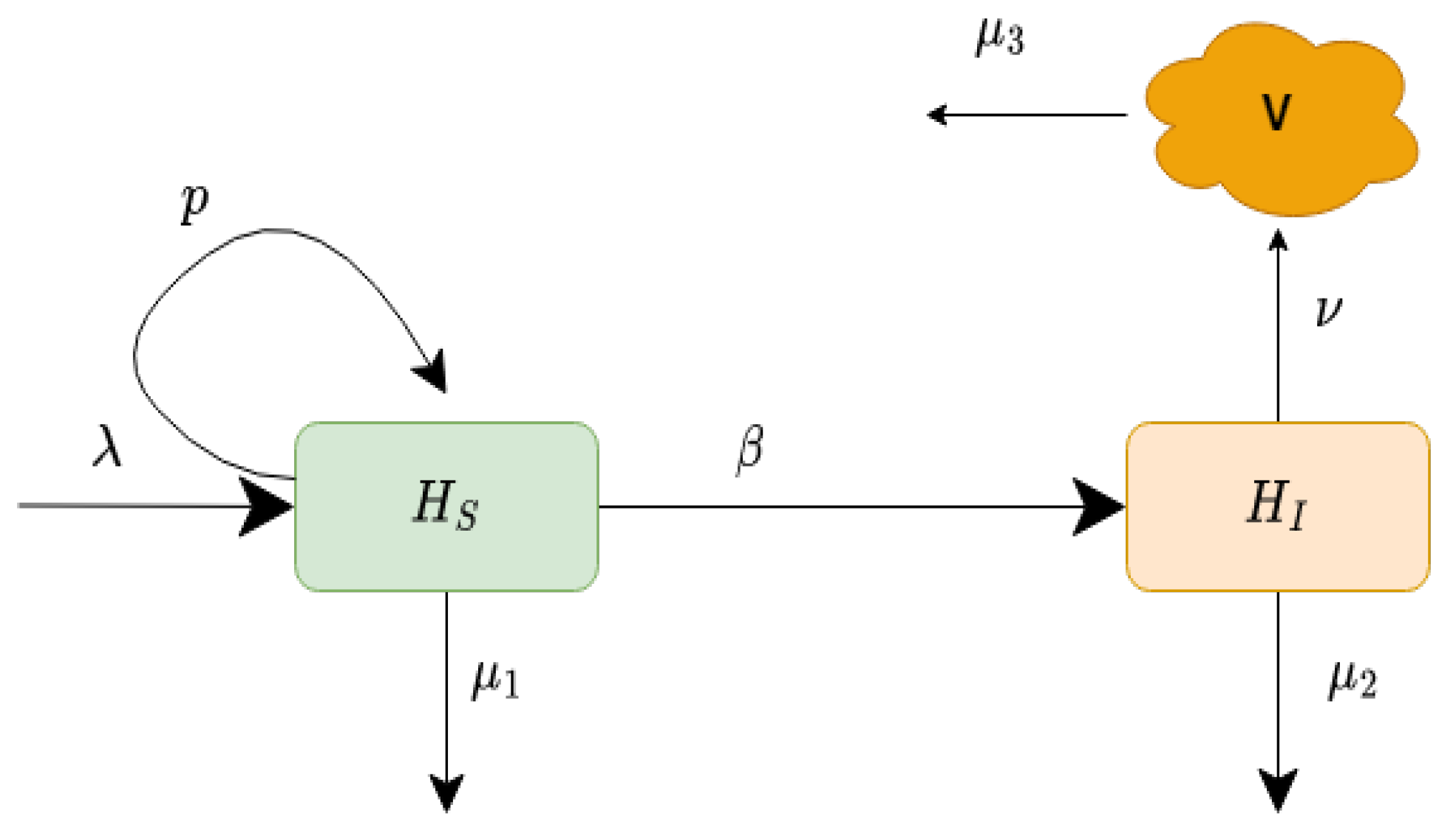
In this model, is the constant production of healthy liver cells, p is the proliferation rate at which the new cells are produced from the existing cells, is the maximum value of liver cells at which proliferation stops, is the rate of transmission, is the death rate of uninfected liver cells, is the death rate of infected liver cells, is the production rate of new virions, and is the removal rate of the virus. The schematic explanation of our proposed model is displayed in Figure 1. The values of the parameters of model (1) are given in Table 1.

Figure 1.
Schematic diagram of the infection process of the model (1).

Table 1.
List of parameters for the model (1).
3. Well-Posedness of the Model
3.1. Boundedness
We consider the positivity and boundedness of the system (1) with non-negative initial conditions .
Proof.
Observe that
Hence, the system (1) is an invariant set . □
Theorem 2.
Proof.
Using the differential inequality from [23], we obtain
where represents the initial value. As , we have
which means that is the maximum value of the total hepatocyte cells H at time t and thus . Therefore, H will decrease at the extreme level, and hence the hepatocyte cell population is bounded in .
In consequence, we deduce that is the upper bound for □
3.2. Existence Condition
The system (1) has two equilibrium states, which are given below.
- (i)
- The infection-free equilibrium with
- (ii)
- The endemic equilibrium whereand is defined aswithIf and then has a unique positive root. The coefficient if and if and if
Basic Reproduction Number
The local stability of the system is governed by the basic reproduction number . The basic reproduction number is the average number of new secondary infections in entirely susceptible hepatocyte cells produced by a single infected hepatocyte cell. With the help of the next generation method [30], we can calculate the basic reproduction number. For this method, we consider the model variables in such a manner that the compartments reflect only infected individuals. By this assumption, we have , where and V are the two infected compartments. Furthermore, denotes the set of all infection-free states—that is,
System (1) can be rewritten as
where describes the rate of appearance of new infections in compartment i. Moreover,
is the transmission rate into the compartment i, and is the rate of transmission out of this compartment. The subsequent norms are to be modelled.
- ;
- If , then ;
- for ;
- If , then for ;
- For the disease-free equilibrium (DFE) , the Jacobi matrix constrained to the subspace has all negative eigenvalues.
To formulate the next generation matrix [30] from matrices of partial derivatives of and . Specifically,
where . Here, are two-dimensional squared matrices and ( denotes a spectral radius of the matrix). For model (1), we have
Next, we introduce a non-negative matrix F representing the entry of a new infection and a non-singular Metzler matrix V representing the transmission of HCV infection between the infection compartments as follows:
Here, is a non-negative matrix, and therefore is a non-negative next-generation matrix representing the predictable number of new infections, which is given by
Using the spectral radius of the next-generation matrix [30,33], for the system (1), we find the basic reproduction number , which is the largest eigenvalue of at . Thus,
3.3. Stability of the System
Theorem 4.
To verify the local stability of the system (1) at , the Jacobian matrix is given by
Now, at the infection-free equilibrium of system (1), the Jacobian is
and the characteristic equation for (23) is
Now, it is easy to note that , and . If , then all the roots of Equation (25) will be negative (Section 3.3 in [33]). If , then we have threshold criteria to determine the stability condition at the infection-free point . We have the condition , which implies that and results in the eradication of infection. Hence, we find the following theorem.
Theorem 5.
For , the infection-free equilibrium is locally asymptotically stable and unstable otherwise.
Remark 1.
The infection-free state exists when , and the system switches to its infection-free state if .
Theorem 6.
The system (1) around is locally asymptotically stable (LAS) if .
Proof.
We already established that the equilibrium is feasible when . Now, the Jacobi matrix around is
where
At , the characteristic equation is
where
By the Routh–Hurwitz criteria at the endemic equilibrium , the system is LAS if . □
3.4. Global Stability
Theorem 7.
The system is globally asymptotically stable (GAS) when .
Proof.
We consider the Lyapunov function as follows:
When , we have and implies that . From the model (1), we can say that when in the limit . Hence, according to the Lyapunov–LaSalle theorem, the system is globally asymptotically stable when . This completes the proof. □
Theorem 8.
The endemic equilibrium is globally asymptotically stable (GAS) if
Proof.
Let us consider the Dulac function:
and denote the right-hand side of equations in the system (1) as
4. Sensitivity Analysis
Sensitivity analysis is useful to explore the effect of fluctuations and relative changes in the parameters associated with the basic reproduction number. Here, we perform a sensitivity analysis to study the influence of model parameters on the basic reproduction number in the transmission of HCV infection.
It is clear from the expression (21) of the threshold quantity () of model (1) that it is a combination of various epidemic parameters. We use a formula given in [33] to calculate the sensitivity indices of every epidemic parameter to the disease transmission. In this analysis, we can easily quantify the parameters that are more sensitive to disease transmission and control by analysing a control mechanism program to eliminate the infection from human livers.
Now, we proceed to give the forward sensitivity indices of with respect to the model parameters by considering the formula:
Using the above sensitivity index formula, we have
If the sensitivity index is positive, then will increase with the increasing value of the corresponding parameters. If decreases with the increasing value of the parameter, the sensitivity index of the corresponding parameter will also become negative. For the parameters and p, the sensitivity indices are plotted in Figure 2. The sensitivity indices in Table 2 and Figure 2 suggest that HCV infection control can be achieved by reducing the values of . Furthermore, the parameters and have an inverse effect on reducing the infection level.
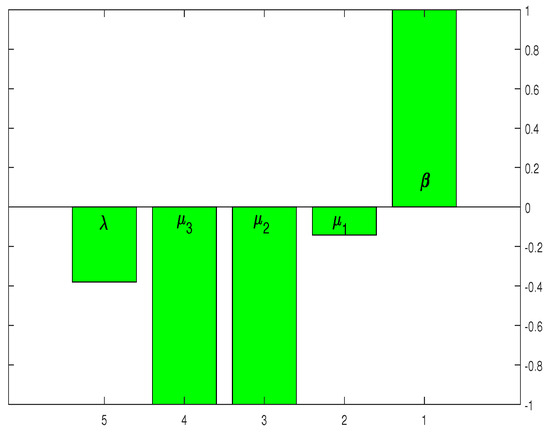
Figure 2.
Graphical representation of the outcome in Table 2.
Table 2.
The parameters and the associated sensitivity indices along with the relative percentage impact on the threshold quantity ().
Numerical Findings of the System (1)
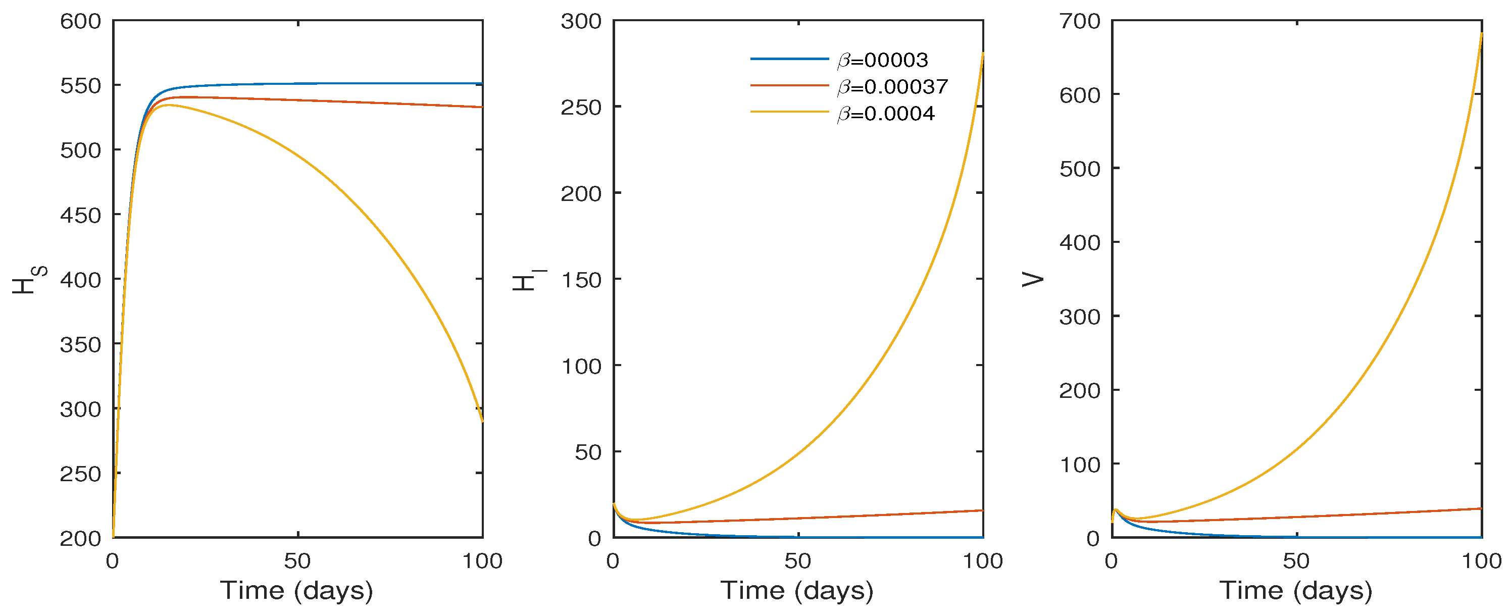
In this subsection, the findings of the numerical simulation are performed for the cellular level HCV model given in Equation (1). We tested the effect of the , the transmission rate (see Figure 3), and p, the proliferation rate (see Figure 4), using ode45. The parameter values in Table 1 were used for the numerical simulation. The numerical simulation provides better comprehension of the effect of parameters on the system dynamics. Figure 3 shows that the basic reproduction number changes to when , and the system becomes infection-free. If the value of increases, the basic reproduction number increases to , and the system moves to an endemic state. On the other hand, if the proliferation rate p increases from to , the system switches from an endemic state to an infection-free state.
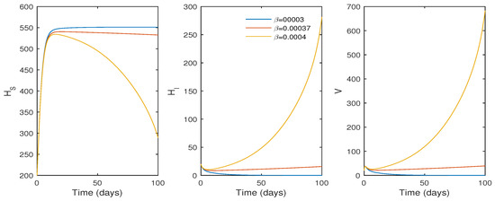
Figure 3.
The effect of the infection rate () on the system trajectories with and ; time t in days; and the values of the parameters as given in Table 1.
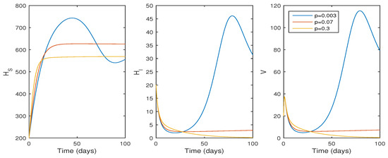
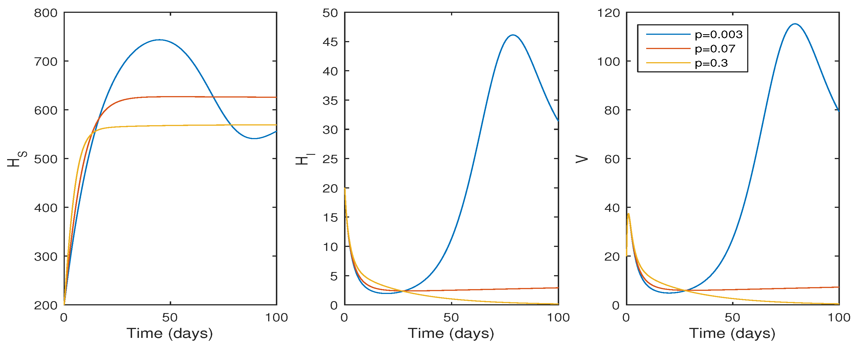
Figure 4.
The effect of infection rate (p) on system trajectories with and ; time t in days; and the values of the parameters as given in Table 1.
Biologically, it suggests that an increasing proliferation rate can only control the infection rate to a certain extent. According to the simulation results, the basic reproduction number increases as increases, and a value of results in . Thus, a reduced disease transmission rate must help to minimize the HCV infection and the infection level moves to extinction if decreases.
According to Figure 4, if the proliferation rate decreases, the infection cell level and viral load increase, whereas the viral load and infected cell level decrease if , and the system switches to its infection-free state as . Biologically, this suggests that the HCV infection decreases whenever the liver cell proliferation rate increases, and the infection is eradicated from the system whenever .
Figure 2 shows that the highest sensitivity indexes are , and with sensitivity indices of , and . The sensitivity index of suggests that the threshold quantity also rises by as the parameter value grows by as shown in Figure 2. Similarly, increasing the values of and by would decrease the threshold measure by . The sensitivity analysis and Figure 2 indicate that some mechanism is required to control the parameter threshold values as much as possible.
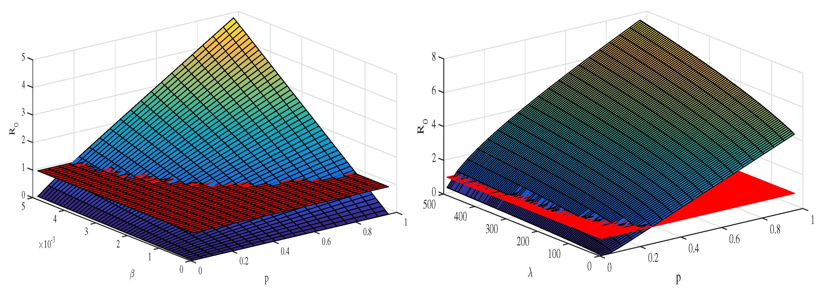
Figure 5 depicts the mesh plot of with respect to and p (left panel) and with respect to and p (right panel). In this case, we can define a control model to optimize the value of this quantity in light of the sensitivity analysis in the next section.
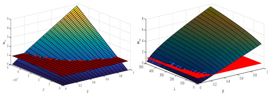
Figure 5.
The plots depict the sensitivity analysis of the threshold quantity () and its relative impact as various epidemic parameters vary. The left panel depicts how the value of the basic reproduction number changes when the disease transmission rate and the proliferation rate p vary concurrently. The right panel shows how changes when the disease transmission rate () and production rate () vary at the same time. The values of the parameters are the same as given in Table 1.
5. Optimal Control Problem
Optimal control theory is a useful technique to develop various control strategies for the minimization of different infectious diseases [6,18,34]. Here, the major focus is on reducing the viral load and the infected liver cell count. On the basis of the sensitivity analysis of the threshold parameter, we modelled the control problem. The combination of control inputs is defined as . Physically or biologically, these control measures represent the control of new infections and new virus production from infected liver cells.
The control parameters or variables in the proposed model (1), lead to the following control problem:
subject to the modified form of the system (1) given by
complemented with the initial conditions:
In the objective functional described by (39), and and D are the positive constants called as weight constants. The weight constants C and D are the relative cost of infected and virus, while A and B are the weight constants measuring the associated cost of the control variables and , respectively. The goal of our control problem (39) is to eradicate the disease on the basis of minimizing the infected population and reservoir and increasing the ratio of the recovered population by considering the control measure cost. We find the control function represented by as
subject to the control system (39) and (40), where denotes the set of control functions described by the following equation
We first show the existence of such control measure variables. Following the idea demonstrated in [35] that the existence of solution for a system is subjected to the boundedness of the controls as they are the Lebesgue measure and the non-negativity of the initial data.Thus, the control problem can be expressed in the following form:
where and the matrices A and , respectively, containing the linear and nonlinear bounded coefficients are given by
and
Setting and noting that
where is free of the model state variables, we have
with , which shows that the function is uniformly continuous and Lipschitz. Clearly, and are all non-negative quantities and ensure the existence of a solution for the model (40).
The following theorem deals with the existence of a solution to the control system described by (40) and (41).
Theorem 9.
There exists an optimal solution to the control problem (40).
Proof.
Clearly, the state and control variables have non-negative values. Furthermore, the set of control is closed and convex. Moreover, the boundedness of the control system leads to its compactness. The integral functional (39) is also convex. Therefore, optimal controls exist. □
5.1. Methodology
Let the control input denote the quantity of the drug dose at time t. The cost function (39) subject to the system of ODE (40) represents the necessary conditions for which an optimal control and corresponding states must satisfy Pontryagin’s Maximum Principle. To determine the optimal control and , we use Pontryagin’s maximum principle [36]. With the aid of this principle, we change the system (40) and the cost function (39) into a minimizing problem by constructing the Hamiltonian function H with respect to .
We find the optimal values to the problem described by (39) subject to the control system (40). For that, the Lagrangian, as well as the Hamiltonian associated with the control problem, will be defined. Therefore, we take the state variable x and control variable u to define the Lagrangian () as
Using the adjoint variables together with the state variables, the Hamiltonian is constructed as follows:
Here, denote the adjoint variables, P and Q are the weight constants, and A represents the penalty multiplier.
From (49), we have
The adjoint system to be estimated for the control input associated with the model state variables is represented as
Here, the transversality conditions are According to Pontryagin’s Maximum Principle [36], the optimal control satisfies
From the last two equations of (50), we have
Solving (53) for and , we obtain
Since the standard control is bounded, we conclude that
The compact form of is
Similarly, the compact form of is
Considering (39) and (40), the state system together with the adjoint system and the transversality conditions, we find the following optimal system:
The graphical presentation of the application of the control analysis is better understood than the corresponding analytic findings. Therefore, we proceed for the numerical investigation of the control analysis in the next section.
5.2. Numerical Findings of the Control System
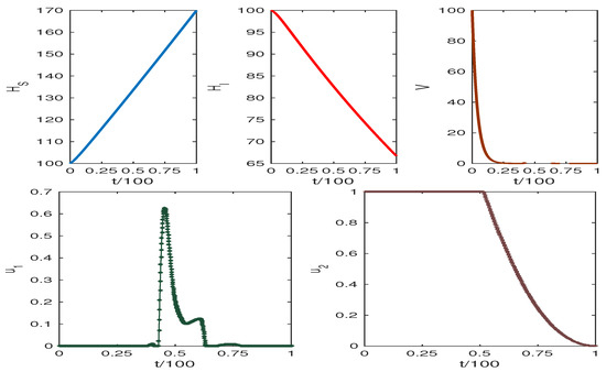
We describe the application of our control strategies graphically by applying the Runge–Kutta method of the fourth order for the numerical simulation. We assume the numerical values given in Table 1. The adjoint and the state systems are solved with the aid of the backward Runge–Kutta method of the fourth order with the transversality conditions.
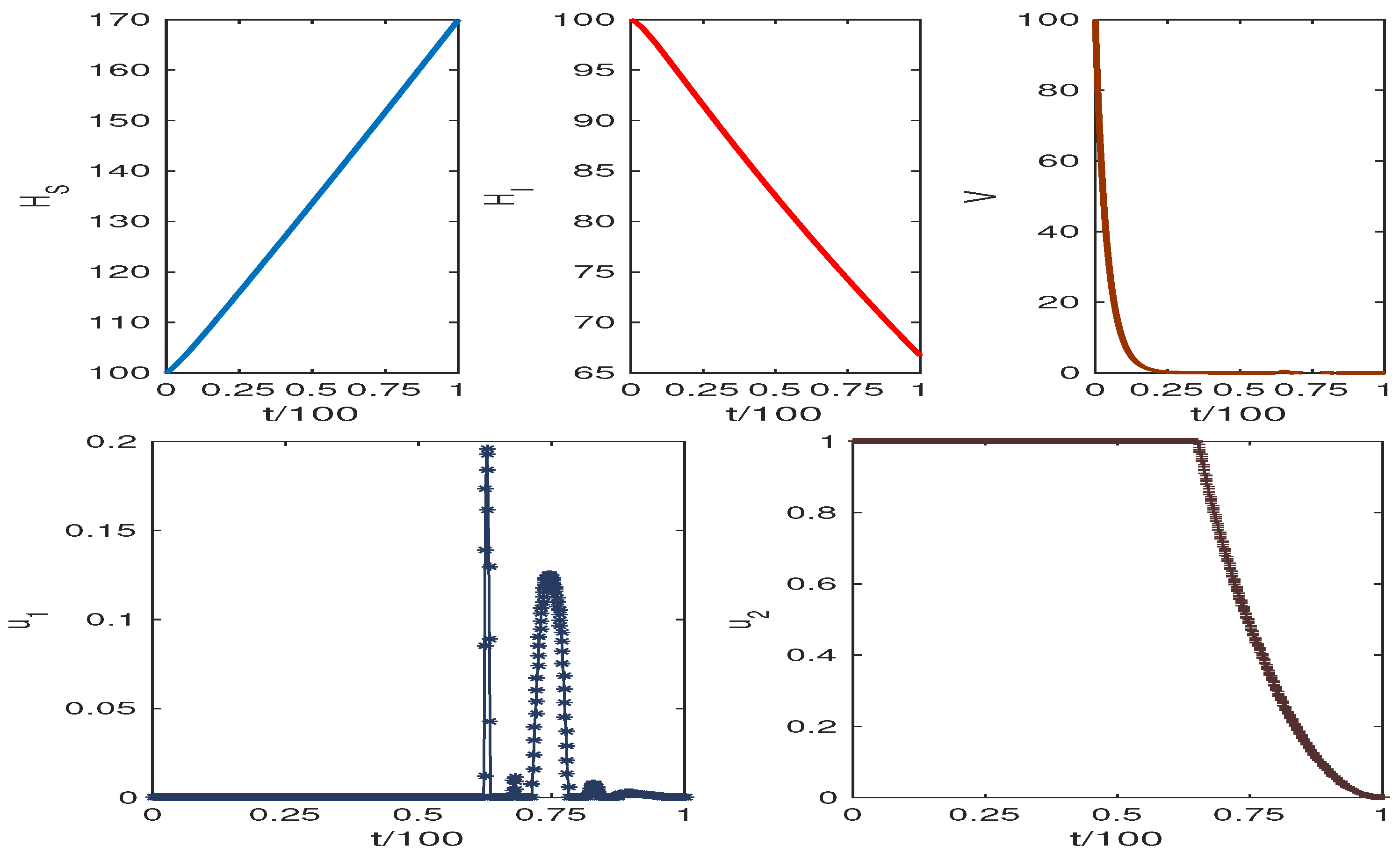
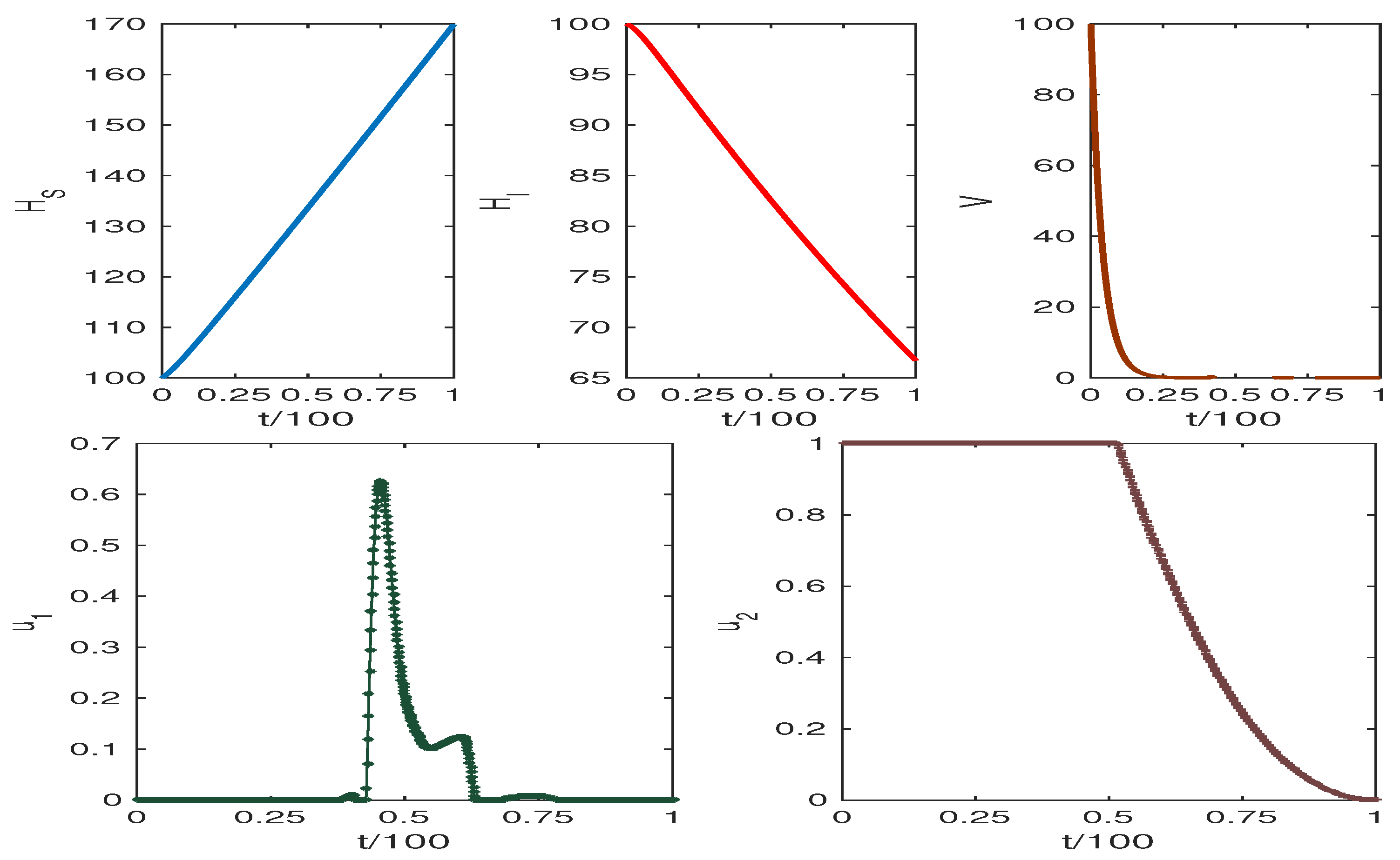
The obtained results are presented in Figure 6 and Figure 7. The weight factors for Figure 6 and Figure 7 are taken from the table. The graphics clearly show our target to reduce the infected cell populations and viral load and the effect of control analysis. Thus, we conclude that our control mechanism leads to avoiding the death case of HCV infection.

6. Discussion
In this study, we proposed a three-dimensional compartmental model for the cellular dynamics of HCV infection with control measures for drug control. Both analytic and numerical studies of the HCV infection model were performed to evaluate the effect of various controlling strategies on the dynamics of the disease. The analysis of our proposed mathematical model contains theoretical as well as numerical findings. The infection-free state exists when the basic reproduction number is less than unity. In this case, the endemic equilibrium does not exist.
When the corresponding reproduction number is less than unity, the infection-free equilibrium point of the HCV infection model is shown to be globally asymptotically stable. The infection-free equilibrium of the model is shown to be locally asymptotically stable when the corresponding basic reproduction number is less than unity, and the endemic equilibrium is shown to be locally asymptotically stable when the corresponding basic reproduction number is greater than unity and unstable otherwise.
The sensitivity analysis of our model reveals that the HCV transmission rate , the death rate of infected liver cells and the removal rate of virus are more sensitive when is greater than unity and unstable otherwise. The numerical simulation shows that the basic reproduction number for when .
Increasing the value of results in high HCV infection, while the increasing value of p reduces HCV infection. Figure 6 and Figure 7 show the system trajectories in the presence of drug control. The simulation of the trajectories with various weight factors (see Table 3) shows that the uninfected cell population increases, and the infected cell population along with the viral load diminish for the effect of optimal drug control therapy.
Table 3.
The numerical values of the weight constants and initial sizes of the compartmental population.
7. Conclusions
We focused on the role of proliferation during HCV infection in our investigation. Furthermore, the impact of antiviral drug control on the transmission dynamics of HCV infection was studied. We observed that drug-control strategies led to the complete eradication of the HCV viral loads in the system. We can extend this model by considering the latent class of infected cells. Furthermore, the wild and mutant virus classes can be considered to obtain a complete understanding of the infection process. Of course, we cannot take into account all such considerations in order to avoid complexity. However, we plan to consider these options in our future work.
Author Contributions
Each of the authors, S.K.S., A.N.C. and B.A., contributed equally to each part of this work. All authors have read and agreed to the published version of the manuscript.
Funding
This research work was funded by Institutional Fund Projects under grant no. (IFPIP: 658-130-1443).
Data Availability Statement
Not applicable.
Acknowledgments
This research work was funded by Institutional Fund Projects under grant no. (IFPIP: 658-130-1443). The authors gratefully acknowledge the technical and financial support provided by the Ministry of Education and King Abdulaziz University, DSR, Jeddah, Saudi Arabia.
Conflicts of Interest
The authors declare that they have no competing interest.
References
- Alvarez, F.; Berg, P.; Bianchi, F.B.; Bianchi, L.; Burroughs, A.; Cancado, E.L.; Chapman, R.; Cooksley, W.; Czaja, A.; Desmet, V.; et al. International Autoimmune Hepatitis Group Report: Review of criteria for diagnosis of autoimmune hepatitis. J. Hepatol. 1999, 31, 929–938. [Google Scholar] [CrossRef]
- Available online: https://www.who.int/news-room/fact-sheets/detail/hepatitis-c (accessed on 24 June 2022).
- Available online: https://www.who.int/news/item/24-06-2022-WHO-publishes-updated-guidance-on-hepatitis-C-infection (accessed on 24 June 2022).
- Sadki, M.; Danane, J.; Allali, K. Hepatitis C virus fractional-order model: Mathematical analysis. Model. Earth Syst. Environ. 2022, 1–13. [Google Scholar] [CrossRef]
- Zitzmann, C.; Kaderali, L.; Perelson, A.S. Mathematical modeling of hepatitis C RNA replication, exosome secretion and virus release. PLoS Comput. Biol. 2020, 16, e1008421. [Google Scholar] [CrossRef] [PubMed]
- Chatterjee, A.N.; Roy, P.K. Anti-viral drug treatment along with immune activator IL-2: A control-based mathematical approach for HIV infection. Int. J. Control 2012, 85, 220–237. [Google Scholar] [CrossRef]
- Chatterjee, A.N.; Singh, M.K.; Kumar, B. The effect of immune responses in HCV disease progression. Eng. Math. Lett. 2019, 2019, 1. [Google Scholar]
- Nowak, M.A.; Bangham, C.R. Population dynamics of immune responses to persistent viruses. Science 1996, 272, 74–79. [Google Scholar] [CrossRef]
- Bonhoeffer, S.; Coffin, J.M.; Nowak, M.A. Human immunodeficiency virus drug therapy and virus load. J. Virol. 1997, 71, 3275–3278. [Google Scholar] [CrossRef]
- Neumann, A.U.; Lam, N.P.; Dahari, H.; Gretch, D.R.; Wiley, T.E.; Layden, T.J.; Perelson, A.S. Hepatitis C viral dynamics in vivo and the antiviral efficacy of interferon-α therapy. Science 1998, 282, 103–107. [Google Scholar] [CrossRef]
- Dahari, H.; Lo, A.; Ribeiro, R.M.; Perelson, A.S. Modeling hepatitis C virus dynamics: Liver regeneration and critical drug efficacy. J. Theor. Biol. 2007, 247, 371–381. [Google Scholar]
- Avendano, R.; Esteva, L.; Flores, J.; Allen, J.F.; Gómez, G.; López-Estrada, J. A mathematical model for the dynamics of hepatitis C. J. Theor. Med. 2002, 4, 109–118. [Google Scholar] [CrossRef]
- Wodarz, D. Hepatitis C virus dynamics and pathology: The role of CTL and antibody responses. J. Gen. Virol. 2003, 84, 1743–1750. [Google Scholar] [CrossRef]
- Dixit, N.M.; Layden-Almer, J.E.; Layden, T.J.; Perelson, A.S. Modelling how ribavirin improves interferon response rates in hepatitis C virus infection. Nature 2004, 432, 922–924. [Google Scholar] [CrossRef] [PubMed]
- Zhao, Y.; Xu, Z. Global dynamics for a delayed hepatitis C virus infection model. Electron. J. Differ. Equ. 2014, 2014, 1–18. [Google Scholar]
- Chatterjee, A.N.; Al Basir, F. Role of immune effector responses during HCV infection: A mathematical study. Math. Anal. Infect. Dis. 2022, 231–245. [Google Scholar] [CrossRef]
- Chatterjee, A.N.; Al Basir, F.; Takeuchi, Y. Effect of DAA therapy in hepatitis C treatment–an impulsive control approach. Math. Biosci. Eng. 2021, 18, 1450–1464. [Google Scholar] [CrossRef] [PubMed]
- Mondal, J.; Samui, P.; Chatterjee, A.N. Effect of SOF/VEL Antiviral Therapy for HCV Treatment. Lett. Biomath. 2021, 8, 191–213. [Google Scholar]
- Echevarria, D.; Gutfraind, A.; Boodram, B.; Major, M.; Del Valle, S.; Cotler, S.J.; Dahari, H. Mathematical modeling of hepatitis C prevalence reduction with antiviral treatment scale-up in persons who inject drugs in metropolitan Chicago. PLoS ONE 2015, 10, e0135901. [Google Scholar] [CrossRef]
- Scott, N.; McBryde, E.; Vickerman, P.; Martin, N.K.; Stone, J.; Drummer, H.; Hellard, M. The role of a hepatitis C virus vaccine: Modelling the benefits alongside direct-acting antiviral treatments. BMC Med. 2015, 13, 1–12. [Google Scholar] [CrossRef]
- Rong, L.; Perelson, A.S. Mathematical analysis of multiscale models for hepatitis C virus dynamics under therapy with direct-acting antiviral agents. Math. Biosci. 2013, 245, 22–30. [Google Scholar] [CrossRef]
- Zhang, S.; Xu, X. Dynamic analysis and optimal control for a model of hepatitis C with treatment. Commun. Nonlinear Sci. Numer. Simul. 2017, 46, 14–25. [Google Scholar] [CrossRef]
- Mattheij, R.; Molenaar, J. Ordinary Differential Equations in Theory and Practice; SIAM: Bangkok, Thailand, 2002. [Google Scholar]
- Ahmed, E.; El-Saka, H. On fractional order models for Hepatitis C. Nonlinear Biomed. Phys. 2010, 4, 1–3. [Google Scholar] [CrossRef]
- Yang, X.; Chen, L.; Chen, J. Permanence and positive periodic solution for the single-species nonautonomous delay diffusive models. Comput. Math. Appl. 1996, 32, 109–116. [Google Scholar] [CrossRef]
- Guedj, J.; Neumann, A. Understanding hepatitis C viral dynamics with direct-acting antiviral agents due to the interplay between intracellular replication and cellular infection dynamics. J. Theor. Biol. 2010, 267, 330–340. [Google Scholar] [CrossRef]
- De Clercq, E. Current race in the development of DAAs (direct-acting antivirals) against HCV. Biochem. Pharmacol. 2014, 89, 441–452. [Google Scholar] [CrossRef]
- Das, D.; Pandya, M. Recent advancement of direct-acting antiviral agents (DAAs) in hepatitis C therapy. Mini Rev. Med. Chem. 2018, 18, 584–596. [Google Scholar] [CrossRef]
- Mogalian, E.; German, P.; Kearney, B.P.; Yang, C.Y.; Brainard, D.; Link, J.; McNally, J.; Han, L.; Ling, J.; Mathias, A. Preclinical pharmacokinetics and first-in-human pharmacokinetics, safety, and tolerability of velpatasvir, a pangenotypic hepatitis C virus NS5A inhibitor, in healthy subjects. Antimicrob. Agents Chemother. 2017, 61, e02084-16. [Google Scholar] [CrossRef]
- Van den Driessche, P.; Watmough, J. Reproduction numbers and sub-threshold endemic equilibria for compartmental models of disease transmission. Math. Biosci. 2002, 180, 29–48. [Google Scholar] [CrossRef]
- Lawitz, E.J.; Dvory-Sobol, H.; Doehle, B.P.; Worth, A.S.; McNally, J.; Brainard, D.M.; Link, J.O.; Miller, M.D.; Mo, H. Clinical resistance to velpatasvir (GS-5816), a novel pan-genotypic inhibitor of the hepatitis C virus NS5A protein. Antimicrob. Agents Chemother. 2016, 60, 5368–5378. [Google Scholar] [CrossRef]
- Younossi, Z.M.; Stepanova, M.; Feld, J.; Zeuzem, S.; Sulkowski, M.; Foster, G.R.; Mangia, A.; Charlton, M.; O’Leary, J.G.; Curry, M.P.; et al. Sofosbuvir and velpatasvir combination improves patient-reported outcomes for patients with HCV infection, without or with compensated or decompensated cirrhosis. Clin. Gastroenterol. Hepatol. 2017, 15, 421–430. [Google Scholar] [CrossRef]
- Heffernan, J.M.; Smith, R.J.; Wahl, L.M. Perspectives on the basic reproductive ratio. J. R. Soc. Interface 2005, 2, 281–293. [Google Scholar] [CrossRef]
- Ghosh, S.; Chatterjee, A.; Roy, P.; Grigorenko, N.; Khailov, E.; Grigorieva, E. Mathematical Modeling and Control of the Cell Dynamics in Leprosy. Comput. Math. Model. 2021, 32, 52–74. [Google Scholar] [CrossRef]
- Lukes, D.L. Differential Equations: Classical to Controlled; Academic Press: Cambridge, MA, USA, 1982. [Google Scholar]
- Pontryagin, L.S. Mathematical Theory of Optimal Processes; CRC Press: Boca Raton, FL, USA, 1987. [Google Scholar]

Disclaimer/Publisher’s Note: The statements, opinions and data contained in all publications are solely those of the individual author(s) and contributor(s) and not of MDPI and/or the editor(s). MDPI and/or the editor(s) disclaim responsibility for any injury to people or property resulting from any ideas, methods, instructions or products referred to in the content. |
© 2023 by the authors. Licensee MDPI, Basel, Switzerland. This article is an open access article distributed under the terms and conditions of the Creative Commons Attribution (CC BY) license (https://creativecommons.org/licenses/by/4.0/).