Expected Waiting Times at an Intersection with a Green Extension Strategy for Freight Vehicles: An Analytical Analysis

Abstract

The need for transporting commodities has led to more and more freight vehicles on urban roads. Specific operational constraints of such vehicles could induce non-homogeneities in the smooth movement of traffic, especially at intersections where acceleration/deceleration events occur frequently. This leads to unnecessary wasted time for all vehicles, even in low to moderate traffic conditions. Hence, the literature reports different proposals to enhance the continuity of traffic at intersections. Among them, the green extension strategy has attracted researchers’ attention, owing to its simplicity, flexibility and practicality. In this paper, we propose a new approximate probabilistic model for the expected waiting/wasted time of all vehicles at an intersection with green time extension in low to moderate traffic conditions. Accordingly, the optimal green extension interval that minimizes the total expected waiting time can then be determined in different conditions. The proposed analysis needs few pieces of information (as opposed to microsimulation models conventionally employed to analyze such systems) and is therefore, suitable for quickly deciding on the optimal strategy based on the current situation in a dynamic environment. We have validated our approximate analysis with simulations in the VISSIM simulation tool.

1. Introduction

Freight transport has been playing an important role in connecting producers and consumers in all sectors around the world [1]. However, as shown in recent work (e.g., [2]), mixed freight and regular traffic is susceptible to inconsistencies, resulting in an inefficient applications of traditional traffic control methods, especially at intersections, which are known to be the bottlenecks of traffic systems [3]. Hence, given the increasing number of freight vehicles in traffic streams, experts have been looking vigorously for new control methods capable of addressing the concomitant challenges. Specifically, it has been found that the frequency of decelerations and accelerations of freight vehicles is one of the most important challenges aggravating traffic congestion [4,5]. Accordingly, the proposal of new strategies for alleviating such problems by reducing stop-and-go events of freight vehicles has attracted the attention of researchers.

In the case of a signalized intersection, stop-and-go events of freight vehicles can lead to unnecessary waiting times for all vehicles, even in undersaturated conditions. In this regard, methods modifying green time duration when freight vehicles or any other type of special vehicle are arriving are among the most promising strategies due to their simplicity, efficiency and alignment with traditional pre-timed signals. From the traffic control point of view, special vehicles are defined as vehicles with higher priority with respect to their nature (e.g., emergency vehicles) or considering their operational constraints (e.g., freight vehicles, trucks and buses). Instances of such methods are collectively referred to as green extension models because they generally extend the green time if there is an arriving freight vehicle [6]. There are other models, namely, early green models [7], which (to a large extent) follow the same strategy to give priority to a certain class of vehicles. This means that green time is extended with a predetermined interval if a freight vehicle arrives in that interval, independently of the waiting vehicles in conflicting streams.

Given the above-explained setting of such a model, there is thus a need to study the influence of and derive the optimum of extension intervals for given conditions of the intersection. To this end, employing laboratory evaluations such as (micro)simulations, whose high elaboration level leads to the traffic representation, as would be observed in reality, has been a popular solution [8,9,10]. However, taking all microscopic factors into account renders this approach computationally intensive with adverse effects on generalizability and applicability [11]. Accordingly, introducing an analytical model for such a purpose could be a better option [12], due to its simplicity and suitability for iteratively calculating the optimal extension interval in dynamic conditions.

Motivated by this fact, mathematical techniques are also used (yet relatively much more sparse) to represent the progress of traffic flow at intersections to eventually evaluate the implications of a green extension model. Although the incorporation of all underlying uncertainties present in traffic is difficult to achieve by analytic models [13], by imposing plausible assumptions, one can construct analytical, differentiable and computationally tractable approximations for the performance indices, including delay and queue length [14,15,16].

With this paper, we want to add to the literature on analytic models for intersections. More precisely, we propose a simple stochastic model to calculate the mean waiting (or wasted) time of all vehicle streams at an undersaturated signalized intersection, where an arbitrary number of green time groups have the ability to extend green time if a freight vehicle arrives. Here, a green time group is defined as a collection of lanes that receive a green signal simultaneously, i.e., that are non-conflicting. During a cycle, it is assumed that all green time groups receive a green signal sequentially in some specified order. The waiting time of a vehicle is defined as the extra time that the vehicle needs if it has to slow down or stop because either the traffic light is red or the overflow queue built up during the previous red time has not dissipated yet. We approximate the mean waiting time of a regular or freight vehicle arriving in any lane of the intersection, taking into account the possible green time extensions, the presence of freight vehicles, the lengths of the vehicles, their speeds, the stochastic nature of arrivals, etc. We assume that all vehicles that have arrived during a red period can leave the intersection during their next regular green period(s). Although this assumption does not hold in reality, due to the stochastic nature of traffic, imposing this assumption considerably simplifies the calculations, but according to the results of our validation, it negligibly affects the results in a light-traffic (undersaturated) scenario. We stress here that the problem we deal with is interesting in light-traffic (to moderate-traffic) scenarios anyway, since in heavy-traffic scenarios the overall load (rather than avoidable stop-and-go events of freight vehicles) causes congestion. Therefore, we expect the most gains from green time extensions in (relatively) light-traffic scenarios.

With these approximations of the mean waiting time, the influence of the lengths of green time extensions can be studied, along with their optimal values. We therefore, include an extensive number of numerical examples for a simple intersection with two green time groups with one having a green time extension possibility. For validation, we have also developed an internal script to simulate the provided numerical example in VISSIM. The simulation results confirm that the proposed approximations represent a good compromise between accuracy and efficiency, and work sufficiently well.

This paper is structured as follows. This section is followed by a brief review of related studies in Section 2. Section 3 describes the structure of the proposed analysis. Section 4 provides a numerical example, along with the associated simulation. Finally, Section 5 closes this paper by enumerating the main conclusions and giving an outlook for future work.

2. Related Work

Before proceeding to review the relevant literature, it is worth mentioning that this research focuses on proposing a mathematical technique to model intersections with green time extension in a light-traffic scenario, and this section is limited to this scope accordingly. However, interested readers can find:

• a comprehensive survey on similar models based on simulation approaches in [13,17,18,19];
• a review of more advanced traffic signal control strategies in [20,21,22,23];
• an introduction to vehicles’ motion prediction/optimization in intersection control in [5,24,25];
• the incorporation of traffic heterogeneity (in terms of either drivers or vehicles) into traffic prediction and control in [26,27,28].

In this section, we review the related literature on transit and freight signal priority with a focus on mathematical models and non-saturated traffic conditions.

In [29], the evaluation of transit signal priority is carried out based on the delay equation proposed in the highway capacity manual (HCM) [30]. By doing so, the optimal transit signal plan could be determined based on an objective function, aiming to minimize the average delay of the transit vehicles subject to the deterministic estimation of the HCM equation. Following the same (deterministic) scheme, the authors of [31] proposed a methodology to calculate the experienced delay of buses in the case of a bus preemption strategy. Using the proposed calculations, the study then recommended a careful selection of design parameters to have a more beneficial system. However, the consequences of such a system on the traffic flow of side roads constitute an important issue overlooked in that study.

Lin [32] paid particular attention to how the green extension strategy affects the flow of traffic on the side roads. They found that such effects are too important to be neglected. However, this study failed to address the uncertainties in the arrivals of buses and their positions in the queue. Similarly, in [12], the authors assumed that the operation of green extension strategies does not significantly depend on the randomness of traffic streams. Accordingly, they utilized a deterministic queuing model to evaluate the impact of such a system on the expected delay. Under the same assumptions, ref. [11] developed an analytical model by assuming deterministic inter-arrival and service times to evaluate the deployment of extended green time systems. Accordingly, they identified intersection geometry, signal timings and traffic demands, to name only a few, as the contributing factors affecting the performances of systems of this type. However, stochasticity and the optimal extension interval still remained unaddressed.

This paper is an extension of [33], where a stochastic model was introduced for a simple intersection. The current paper extends this to a much more general setting of intersection architecture and possibilities of green extensions for different lanes. The optimal extension intervals for different conditions are also calculated (numerically). Finally, comparison of the obtained results to those of the associated simulations is added and validates the analytic analysis.

3. The Analysis of the Expected Waiting Times

Before carrying out the analysis of the expected waiting times of all types of vehicles on all lanes, we clarify the notation used in this paper. We assume that the traffic streams traversing the intersection can be divided into green time groups, where all streams in a green time group have a green signal simultaneously. We assume an intersection with a general number (m) of different green time groups. To analyze this general model, we have imposed the following assumptions:

• The green time of a green time group can either be extended if a freight vehicle arrives during the green extension period or cannot. This is designed beforehand. $S_{eg}$ is defined as the set of all green time groups that can extend their green time and $Q_{eg}$ as the set of all subsets of $S_{eg}$.
• Considering a certain green time group i, the extended green interval (if extension is possible), regular red and green times are indicated by $t_{eg,i}$, $t_{r,i}$ and $t_{g,i}$, respectively, (all in terms of seconds). Regular red and green times are the periods when no green time group would have green extension. These times can not all be chosen independently, as for instance, $t_{r,i}$ is equal to ${\sum }_{j\ne i}{t}_{g,j}$ plus lost time. In that respect, an extended green time of one green time group augments the red times of the other green time groups.
• We assume an undersaturated intersection. Therefore, we assume that arrivals of regular (index n) and freight vehicles (index f) in lane l of green time group i are independent Poisson processes (which can describe isolated intersections) with flow rates ${\lambda }_{n,i,l}$ and ${\lambda }_{f,i,l}$ (veh/s), respectively.
• If a vehicle does not have to stop at the intersection (because of a green phase and no queuing), its waiting time is assumed to be zero. However, if a vehicle has to stop, its waiting time is assumed to be the remaining red time (if any) and the time needed to pass the traffic light when the light turns green. After a stop-and-go event, we assume that regular vehicles and freight vehicles drive at constant speeds of $v_n$ and $v_f$ (m/s), respectively. We assume that $v_f<v_n$. We do not consider accelerations, but we do assume that the dissipation speed of queues depends on the presence of freight vehicles in the queue.
• A regular vehicle occupies $l_n$, and a freight vehicle occupies $l_f$, meters of the road after stopping at the traffic light.
• We do not have overflow queues (i.e., all vehicles that arrived during a red period are assumed to leave the intersection during the next regular green period).
• For the analysis of the waiting times of vehicles in green time group i, we define a cycle for green time group i in such a way that each cycle ends with a regular green period for that green time group. By doing so, if the green period is extended, we regard the extension of that green period to be the start of the next cycle. For our analysis, this is the most natural assumption, but other definitions are possible as well, e.g., where the extension of a green period is still part of the previous cycle. Although this could lead to slightly different approximative results, we expect no big influence of this modeling choice.
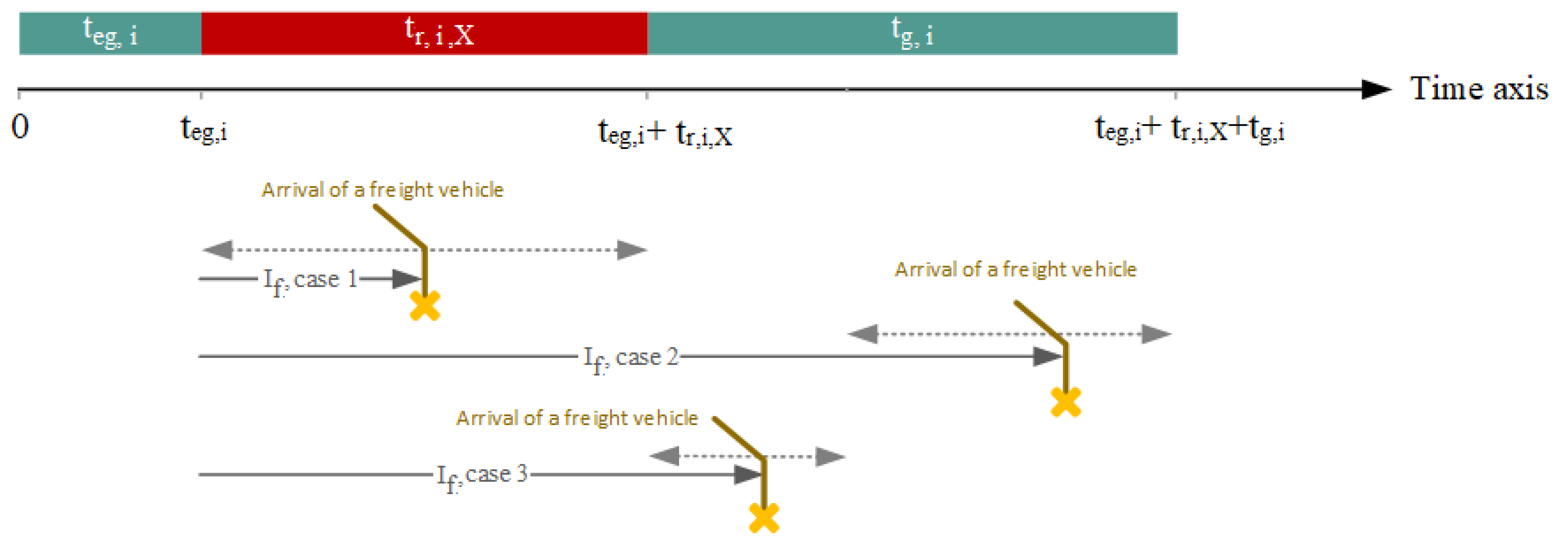
• We define $\mathrm{Pr}\left[E{G}_i\right]$ as the probability that a random cycle of green time group i, that has extension possibility, experiences a green extension of that green time group (in other words, a freight vehicle in green time group i arrives at the intersection during the green extension period). Recall that freight vehicles arrive according to Poisson processes and each green time group i consists of a number of lanes with arrival rates ${\lambda }_{f,i,l}$ (for each lane l) for freight vehicles that all can cause green extension for the green time group. By taking these considerations into account and using properties of the Poisson processes, $\mathrm{Pr}\left[E{G}_i\right]$ can be expressed as:

  $$\begin{array}{c}\hfill \mathrm{Pr}\left[E{G}_i\right]=1-\exp (-(\sum _{l\in M_i}{\lambda }_{f,i,l})t_{eg,i}),\end{array}$$

  (1)

  where $M_i$ is the set of lanes of green time group i.

Under these assumptions, we propose a general technique for calculating the expected waiting time of a tagged (regular or freight) vehicle arriving in a particular lane of green time group i. Note that a green time group i without green extension possibility is also included by assuming $t_{eg,i}=0$.

3.1. General Formulation

To calculate the expected waiting time of a category of vehicles that arrive at the intersection in a given lane of green time group i, we randomly tag such a vehicle and the condition on which green time groups are extended in the arrival cycle of this vehicle. The set X in the formulation indicates which green time group(s) is/are extended in the current cycle. Notice that a regular cycle without any green time extensions is also included in the expressions, namely, by the case $X=\varnothing$. Furthermore, $E{C}_{n,i,X}$ ($E{C}_{f,i,X}$) is the event that the tagged regular vehicle (freight vehicle) arrives in a cycle with green time extensions as specified by the set X. Accordingly, the expected waiting time is calculated using the law of total probability:

• Expected waiting time of a tagged regular vehicle arriving in a given lane of green time group i:

  $$\begin{array}{c}\hfill \mathrm{E}\left[W_{n,i}\right]=\sum _{X\in Q_{eg}}\mathrm{Pr}\left[E{C}_{n,i,X}\right]\mathrm{E}\left[W_{n,i}\right|E{C}_{n,i,X}];\end{array}$$

  (2)
• Expected waiting time of a tagged freight vehicle arriving in a given lane of green time group i:

  $$\begin{array}{c}\hfill \mathrm{E}\left[W_{f,i}\right]=\sum _{X\in Q_{eg}}\mathrm{Pr}\left[E{C}_{f,i,X}\right]\mathrm{E}\left[W_{f,i}\right|E{C}_{f,i,X}].\end{array}$$

  (3)

We first calculate the probabilities in Equations (2) and (3). The probability that a tagged regular vehicle in the studied lane of green time group i arrives in a cycle with extensions according to a certain set X can be calculated as

$$\begin{array}{c}\hfill \mathrm{Pr}\left[E{C}_{n,i,X}\right]=\frac{\left[{\prod }_{\begin{array}{c}j\notin X\end{array}}(1-\mathrm{Pr}\left[E{G}_j\right])\right]\left[{\prod }_{\begin{array}{c}k\in X\end{array}}\mathrm{Pr}\left[E{G}_k\right]\right](t_{r,i}+t_{g,i}+{\sum }_{k\in X}{t}_{eg,k})}{t_{r,i}+t_{g,i}+{\sum }_{j\in S_{eg}}\mathrm{Pr}\left[E{G}_j\right]t_{eg,j}}.\end{array}$$

(4)

This equation is an instance of the inspection paradox in renewal theory that links the probability that an event takes place in a certain type of period to the probability that a period of that type is selected. The denominator in this Equation (multiplied by the arrival rate ${\lambda }_{n,i,l}$) refers to the average number of regular vehicles arriving in the studied lane per cycle. The numerator (multiplied by the same constant ${\lambda }_{n,i,l}$) determines the average number of regular vehicles that would arrive in a cycle with green extension for green time groups $k\in X$ (the third factor) multiplied by the probability that the cycle is of the given extension type (the first two factors).

To calculate the probability that a freight vehicle in the studied lane of green time group i arrives in a certain cycle type, a distinction is made between whether or not green time group i is included in X in the given cycle type. If it is included, a freight vehicle that would arrive (from the studied lane) in the first $t_{eg,i}$ seconds of the red period will cause a green time extension itself. Therefore, we have:

$$\begin{array}{cc}\hfill & \mathrm{Pr}\left[E{C}_{f,i,X}\right]=\hfill \\ \hfill & \left\{\begin{array}{cc}\frac{\left[{\prod }_{\begin{array}{c}j\notin X\end{array}}(1-\mathrm{Pr}\left[E{G}_j\right])\right]\left[{\prod }_{\begin{array}{c}k\in X,\\ k\ne i\end{array}}\mathrm{Pr}\left[E{G}_k\right]\right]\left[t_{eg,i}+\mathrm{Pr}\left[E{G}_i\right](t_{r,i}+t_{g,i}+{\sum }_{\begin{array}{c}k\in X,\\ k\ne i\end{array}}{t}_{eg,k})\right]}{t_{r,i}+t_{g,i}+{\sum }_{j\in S_{eg}}\mathrm{Pr}\left[E{G}_j\right]t_{eg,j}},\hfill & \mathrm{if}i\in X\hfill \\ \frac{\left[{\prod }_{\begin{array}{c}j\notin X\end{array}}(1-\mathrm{Pr}\left[E{G}_j\right])\right]\left[{\prod }_{\begin{array}{c}k\in X\end{array}}\mathrm{Pr}\left[E{G}_k\right]\right]\left[(t_{r,i}-t_{eg,i}+t_{g,i}+{\sum }_{k\in X}{t}_{eg,k})\right]}{t_{r,i}+t_{g,i}+{\sum }_{j\in S_{eg}}\mathrm{Pr}\left[E{G}_j\right]t_{eg,j}},\hfill & \mathrm{if}i\notin X\mathrm{or}i\notin S_{eg}.\hfill \end{array}\right.\hfill \end{array}$$

(5)

If green time group i does not have the possibility of a green time extension, Equation (5) simplifies to the second case only.

The proposed formulation (Equations (2) and (3)) further requires the expected waiting time of a tagged vehicle given that it arrives in a cycle with extensions according to X (and this for all X). We summarize all these possible cycle configurations into two generic ones. We (approximately) calculate $\mathrm{E}\left[W_{n,i}\right|E{C}_{n,i,X}]$ and $\mathrm{E}\left[W_{f,i}\right|E{C}_{f,i,X}]$ separately for these two generic configurations, leading to four treated cases in the remainder.

3.2. Different Cases of the Expected Waiting Time in a General Model

We start with the calculation of $\mathrm{E}\left[W_{n,i}\right|E{C}_{n,i,X}]$. We first observe that all extensions of green times of green time groups different from green time group i are just added to the regular red time of green time group i. Therefore, we can analyse all these cases at once by assuming a red time $t_{r,i,X}=t_{r,i}+{\sum }_{k\in X,k\ne i}{t}_{eg,k}$. Secondly, with regard to the possible extension of green time group i itself, we distinguish two cases, namely, cycles where green time group i is extended (i.e., the case where $i\in X$) and cycles where green time group i is not extended (case $i\notin X$). We denote the former by “an extended cycle” and the latter by “a regular cycle”. Summarized, we thus construct formulas for two expected values, denoted, respectively, by $\mathrm{E}\left[W_{n,i}\right|E{C}_{n,i}]$ and $\mathrm{E}\left[W_{n,i}\right|R{C}_{n,i}]$. If $i\in X$ ($i\notin X$), we then use the first (second resp.) formula with $t_{r,i,X}=t_{r,i}+{\sum }_{k\in X,k\ne i}{t}_{eg,k}$ to calculate that particular $\mathrm{E}\left[W_{n,i}\right|E{C}_{n,i,X}]$.

For the calculation of the expected waiting times of freight vehicles arriving in green time group i, we can make similar observations and can therefore also split the calculations into the two cases of an extended and a regular cycle. Therefore, in the remainder, we calculate four expected values for the four different cases.

To simplify notation, we assume that regular and freight vehicles arrive on the studied lane of green time group i according to a Poisson process with rate ${\lambda }_{n,i}$, respectively, ${\lambda }_{f,i}$ veh/s (Note that we only consider the regular vehicles of the same lane as tagged vehicles, since the regular vehicles of the other lanes do not have any impact on the delay of the tagged vehicle. Thus, the notation l in ${\lambda }_{n,i,l}$ is eliminated. Similarly, we denote ${\lambda }_{f,i,l}$ by ${\lambda }_{f,i}$.). Since freight vehicles arriving in lanes of green time group i other than that of the tagged vehicle can also cause green time extension (for instance, from the opposite direction), their arrival rate has an impact as well, and we assume that they arrive according to a Poisson process with rate ${\widehat{\lambda }}_{f,i}$ (which is in fact the sum of the arrival rates of all other lanes in the same green time group as the studied lane).

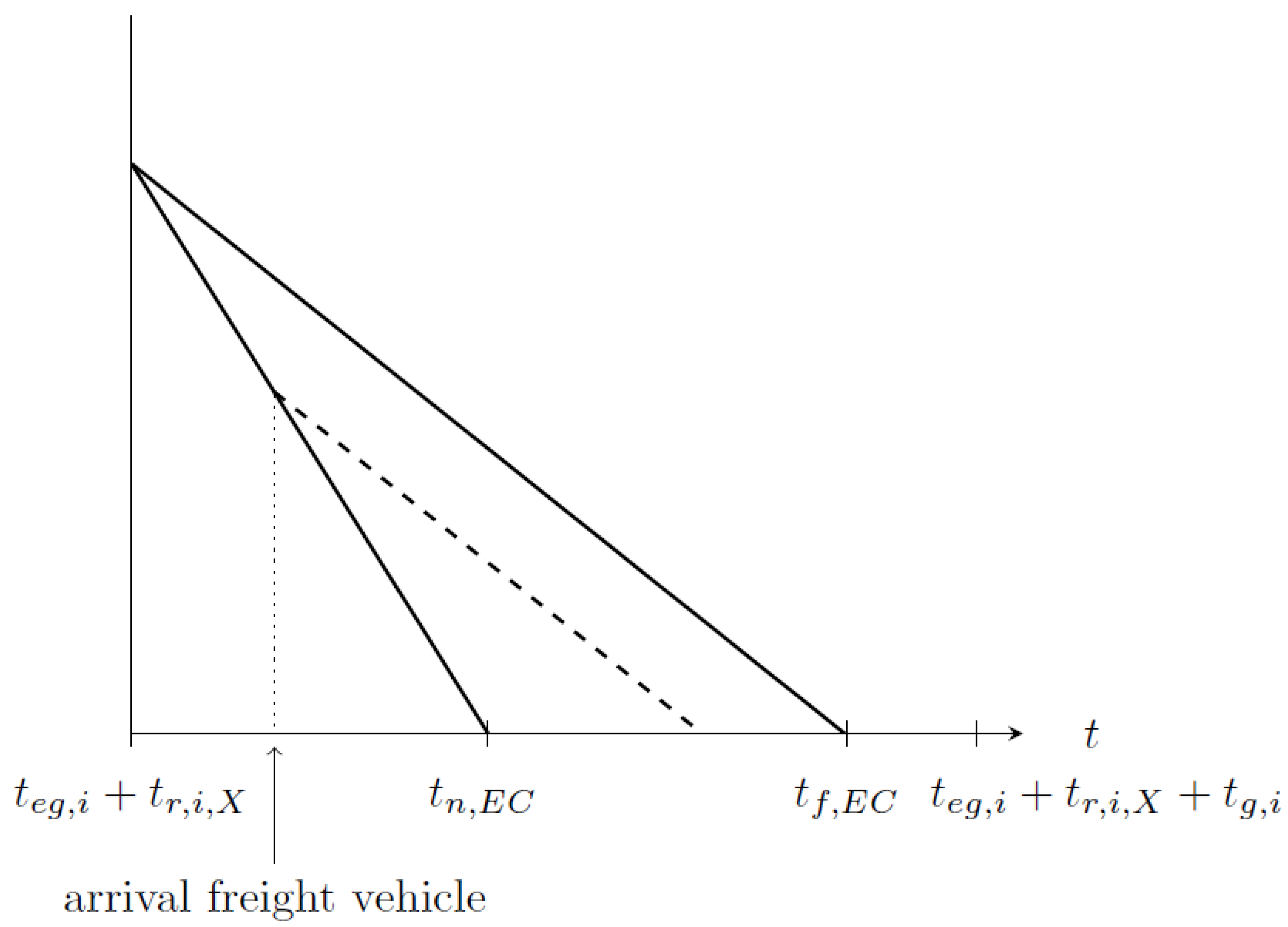
3.2.1. Case 1: Expected Waiting Time of a Tagged Regular Vehicle Arriving in an Extended Cycle

An extended cycle consists of three periods: (in order) the extension interval, the red period and the (regular) green period. We first calculate the expected waiting time with the law of total probability as

$$\begin{array}{c}\hfill \mathrm{E}\left[W_{n,i}\right|E{C}_{n,i}]={\displaystyle \frac{1}{t_{eg,i}+t_{r,i,X}+t_{g,i}}}{\int }_0^{t_{eg,i}+t_{r,i,X}+t_{g,i}}\mathrm{E}\left[W_{n,i}\left(t\right)\right|E{C}_{n,i}]dt,\end{array}$$

(6)

where t is measured from the beginning of the cycle (i.e., $t=0$ corresponds to the start of the cycle), $W_{n,i}\left(t\right)$ is the waiting time of a (regular) vehicle arriving at time t of the cycle and $E{C}_{n,i}$ is the event of the tagged regular vehicle arriving in an extended cycle.

We now first calculate $\mathrm{E}\left[W_{n,i}\left(t\right)\right|E{C}_{n,i}]$. We distinguish three different cases corresponding to the type of period the vehicle arrives in. First, a tagged vehicle arriving during the interval $[0,t_{eg,i}]$ (green extension period) has a waiting time of 0, since we assume no overspill between cycles. Second, if this vehicle arrives at $t\in [t_{eg,i},t_{eg,i}+t_{r,i,X}]$ (red period), the corresponding waiting time consists of (1) the remaining red time and (2) the time that is needed for the acceleration and passing of the traffic light (once it turns green). The latter component depends on the total number of vehicles waiting in front of it and also on whether or not one of them is a freight vehicle. Therefore, by denoting the total number of regular vehicle (freight vehicle) arrivals on the studied lane in an interval of length t by $U_n\left(t\right)$ ($U_f\left(t\right)$, respectively), we can write

$$\begin{array}{cc}\hfill \mathrm{E}\left[W_{n,i}\left(t\right)\right|E{C}_{n,i}]& =(t_{r,i,X}+t_{eg,i}-t)+{\displaystyle \frac{l_f}{v_f}}\mathrm{E}\left[U_f(t-t_{eg,i})\right|E{C}_{n,i}]\hfill \\ \hfill & +{\displaystyle \frac{l_n}{v_n}}\mathrm{E}\left[U_n(t-t_{eg,i})1_{U_f(t-t_{eg,i})=0}\right|E{C}_{n,i}]\hfill \\ \hfill & +{\displaystyle \frac{l_n}{v_f}}\mathrm{E}\left[U_n(t-t_{eg,i})1_{U_f(t-t_{eg,i})>0}\right|E{C}_{n,i}],t\in [t_{eg,i},t_{eg,i}+t_{r,i,X}],\hfill \end{array}$$

(7)

where $1_A$ is the indicator function of event A; i.e., $1_A=1$ if A is true and 0 otherwise. The first term of Equation (7) equals the remaining red time; the second term summarizes the contribution of freight vehicles in front of the tagged vehicle; and the third and fourth terms describe the contribution of the regular vehicles in front of the tagged vehicle when there is no freight vehicle or when there is at least one freight vehicle in front of the tagged vehicle, respectively. The different denominators in these last terms correspond to the different speeds of dissipation of the overflow queue when the light turns green if a freight vehicle is present or if it is not. Under the assumption of Poisson arrivals with rates ${\lambda }_{n,i}$ and ${\lambda }_{f,i}$ for the regular and freight vehicles, Equation (7) is further detailed as:

$$\begin{array}{cc}\hfill \mathrm{E}\left[W_{n,i}\left(t\right)\right|E{C}_{n,i}]& =(t_{r,i,X}+t_{eg,i}-t)+{\displaystyle \frac{l_f}{v_f}}{\lambda }_{f,i}(t-t_{eg,i})\hfill \\ \hfill & +{\lambda }_{n,i}(t-t_{eg,i})\left({\displaystyle \frac{l_n}{v_n}}\exp (-{\lambda }_{f,i}(t-t_{eg,i}))+{\displaystyle \frac{l_n}{v_f}}(1-\exp (-{\lambda }_{f,i}(t-t_{eg,i})))\right)\hfill \\ \hfill & =(t_{r,i,X}+t_{eg,i}-t)+{\displaystyle \frac{[{\lambda }_{n,i}{l}_n+{\lambda }_{f,i}{l}_f](t-t_{eg,i})}{v_f}}\hfill \\ \hfill & -{\lambda }_{n,i}{l}_n\left({\displaystyle \frac{1}{v_f}}-{\displaystyle \frac{1}{v_n}}\right)(t-t_{eg,i})\exp (-{\lambda }_{f,i}(t-t_{eg,i})),t\in [t_{eg,i},t_{eg,i}+t_{r,i,X}].\hfill \end{array}$$

(8)

Third, if the tagged vehicle arrives at $t\in [t_{eg,i}+t_{r,i,X},t_{eg,i}+t_{r,i,X}+t_{g,i}]$ (during a regular green time), the calculation of the corresponding expected waiting time is more complex. We should analyze whether or not the queue formed during the red time has already dissolved at time t, and we should also take the presence of freight vehicles into account. To address these complexities, we propose a simple fluid-flow approximation. In this regard, we assume that

• the queued up vehicles (during the red period) dissolve at a deterministic speed $v_n$ as long as no freight vehicle is present;
• the queue dissolves at speed $v_f$ once a freight vehicle is present;
• newly arriving regular (freight) vehicles each add $l_n$ ($l_f$, respectively) meters to the queue as long as the queue has not completely dissolved;
• when the queue has completely dissolved, it does not build up anymore during the green period (free flow), and the waiting time of newly arriving vehicles will be zero (see also [34]).

We start from the expected queue size at the beginning of the green period and relate the average waiting time of the tagged vehicle arriving at time t to this quantity. To determine the speed at which the queue dissolves during the green time, we need to keep track of the presence of freight vehicles in the queue. We therefore define $I_f$ as the time between the point $t_{eg,i}$ in a cycle and the next arrival instant of a freight vehicle. Accordingly, as is shown in Figure 1, we consider three cases: (1) $I_f\le t_{r,i,X}$: a freight vehicle arrived during the red time of the cycle and the queue dissolves at speed $v_f$ from the start of the following green time; (2) $I_f>t-t_{eg,i}$: no freight vehicle has arrived before time t, and the queue in front of the tagged vehicle dissolves at speed $v_n$; and (3) $t_{r,i,X}<I_f\le t-t_{eg,i}$: no freight vehicle arrived in the red time, but at least one freight vehicle has arrived before time t. The speed of queue dissolving switches from $v_n$ to $v_f$ at the arrival instant of the first freight vehicle in this case. With all this taken into account, we calculate the expected waiting time in the case of $t\in [t_{eg,i}+t_{r,i,X},t_{eg,i}+t_{r,i,X}+t_{g,i}]$ by

$$\begin{array}{cc}\hfill \mathrm{E}\left[W_{n,i}\left(t\right)\right|E{C}_{n,i}]& =\mathrm{E}\left[W_{n,i}\left(t\right)1_{I_f\le t_{r,i,X}}\right|E{C}_{n,i}]+\mathrm{E}\left[W_{n,i}\left(t\right)1_{I_f>t-t_{eg,i}}\right|E{C}_{n,i}]\hfill \\ \hfill & +\mathrm{E}\left[W_{n,i}\left(t\right)1_{t_{r,i,X}<I_f\le t-t_{eg,i}}\right|E{C}_{n,i}],\hfill \end{array}$$

(9)

where each term shows one of the above-enumerated cases. The first term of Equation (9) can be approximated as $\left({(·)}^{+}\stackrel{\Delta }{=}\max (·,0)\right)$

$$\begin{array}{cc}\hfill & \mathrm{E}\left[W_{n,i}\left(t\right)1_{I_f\le t_{r,i,X}}\right|E{C}_{n,i}]\approx \hfill \\ & {\displaystyle \frac{{(\mathrm{E}[l_n{U}_n\left(t_{r,i,X}\right)+l_f{U}_f\left(t_{r,i,X}\right)|E{C}_{n,i},U_f\left(t_{r,i,X}\right)>0]-(v_f-{\lambda }_{f,i}{l}_f-{\lambda }_{n,i}{l}_n)(t-t_{eg,i}-t_{r,i,X}))}^{+}}{v_f}}\hfill \\ \hfill & ·\mathrm{Pr}[I_f\le t_{r,i,X}].\hfill \end{array}$$

(10)

Equation (10) can be understood as follows. The queue size at the start of the green period is determined by the numbers of regular and freight vehicles arriving during the red time and their occupancy lengths. Since at least one freight vehicle arrived during the red period in this case, the queue dissolves during the interval $[t_{eg,i}+t_{r,i,X},t]$ (of length $t-t_{eg,i}-t_{r,i,X}$) before the arrival of the tagged vehicle (taking also new arrivals into account) at a net constant speed of $v_f-{\lambda }_{f,i}{l}_f-{\lambda }_{n,i}{l}_n$; this explains the numerator without the ${\left(\right)}^{+}$-operator. As the arriving vehicle can drive at speed $v_f$ when arriving before dissolution of the queue, its waiting time is obtained by dividing the queue size upon its arrival by the speed $v_f$; this explains the denominator. Finally, the waiting time of the arriving vehicle is zero if the queue has already dissolved at the moment of arrival; this explains the ${\left(\right)}^{+}$-operator. Using the assumption of Poisson arrivals of regular and freight vehicles (which results in an exponential distribution for $I_f$), we can further work out Equation (10) as

$$\begin{array}{cc}\hfill & \mathrm{E}\left[W_{n,i}\left(t\right)1_{I_f\le t_{r,i,X}}\right|E{C}_{n,i}]\approx \hfill \\ & {\displaystyle \frac{{[({\lambda }_{n,i}{l}_n(t-t_{eg,i})-(v_f-{\lambda }_{f,i}{l}_f)(t-t_{eg,i}-t_{r,i,X}))(1-\exp (-{\lambda }_{f,i}{t}_{r,i,X}))+{\lambda }_{f,i}{l}_f{t}_{r,i,X}]}^{+}}{v_f}}.\hfill \end{array}$$

(11)

Similarly, we can approximate the second term of Equation (9) in much the same way, except that no freight vehicles arrive before time t in this case, and the tagged vehicle can drive at speed $v_n$ while crossing the intersection. This results in

$$\begin{array}{cc}\hfill & \mathrm{E}\left[W_{n,i}\left(t\right)1_{I_f>t-t_{eg,i}}\right|E{C}_{n,i}]\approx \hfill \\ \hfill & {\displaystyle \frac{{(\mathrm{E}\left[l_n{U}_n\left(t_{r,i,X}\right)\right|E{C}_{n,i}]-(v_n-{\lambda }_{n,i}{l}_n)(t-t_{eg,i}-t_{r,i,X}))}^{+}}{v_n}}·\mathrm{Pr}[I_f>t-t_{eg,i}],\hfill \end{array}$$

(12)

which can be simplified to

$$\begin{array}{cc}\hfill \mathrm{E}\left[W_{n,i}\left(t\right)1_{I_f>t-t_{eg,i}}\right|E{C}_{n,i}]\approx & {\displaystyle \frac{{[{\lambda }_{n,i}{l}_n(t-t_{eg,i})-v_n(t-t_{eg,i}-t_{r,i,X})]}^{+}}{v_n}}\exp (-{\lambda }_{f,i}(t-t_{eg,i})).\hfill \end{array}$$

(13)

Finally, calculation of the third term of Equation (9) is more intricate. We can write

$$\begin{array}{cc}\hfill & \mathrm{E}\left[W_{n,i}\left(t\right)1_{t_{r,i,X}<I_f\le t-t_{eg,i}}\right|E{C}_{n,i}]\approx \hfill \\ \hfill & {\int }_{t_{r,i,X}}^{\min (t-t_{eg,i},t_{n,EC}-t_{eg,i})}{\displaystyle \frac{{\left(\begin{array}{c}\mathrm{E}\left[l_n{U}_n\left(t_{r,i,X}\right)\right|E{C}_{n,i}]-(v_n-{\lambda }_{n,i}{l}_n)(u-t_{r,i,X})\hfill \\ +l_f-(v_f-{\lambda }_{n,i}{l}_n-{\lambda }_{f,i}{l}_f)(t-t_{eg,i}-u)\hfill \end{array}\right)}^{+}}{v_f}}\hfill \\ \hfill & ·\mathrm{Pr}[u<I_f\le u+du],\hfill \end{array}$$

(14)

since the queue dissolves at net speed $v_n-{\lambda }_{n,i}{l}_n$ until the first freight vehicle arrives and at speed $v_f-{\lambda }_{n,i}{l}_n-{\lambda }_{f,i}{l}_f$ afterwards. This first freight vehicle itself adds $l_f$ meters to the queue, and the tagged regular vehicle arriving at time t can drive at speed $v_f$ m/s if the queue has not dissolved yet. In Equation (14), we need to consider all possible values u for the time $I_f$. To determine the integration interval for u in Equation (14), we first let $t_{n,EC}$ indicate the moment at which the queue would have completely dissolved if it happened at speed $v_n$. Clearly, the integral index u satisfies $t_{r,i,X}<u\le t-t_{eg,i}$. Note, however, that we have to restrict u to $t_{n,EC}-t_{eg,i}$, since the queue is dissolved at $t_{n,EC}$ and freight vehicles arriving after $t_{n,EC}$ do not have to slow down. This explains the min-operator in (14). We can further write:

$$\begin{array}{cc}\hfill \mathrm{E}\left[W_{n,i}\left(t\right)1_{t_{r,i,X}<I_f\le t-t_{eg,i}}\right|E{C}_{n,i}]\approx & {\int }_{t_{r,i,X}}^{\min (t-t_{eg,i},t_{n,EC}-t_{eg,i})}{\lambda }_{f,i}\exp (-{\lambda }_{f,i}u)\hfill \\ \hfill & ·{\displaystyle \frac{{\left(\begin{array}{c}{\lambda }_{n,i}{l}_n(t-t_{eg,i})-v_n(u-t_{r,i,X})+l_f\hfill \\ -(v_f-{\lambda }_{f,i}{l}_f)(t-t_{eg,i}-u)\hfill \end{array}\right)}^{+}}{v_f}}du.\hfill \end{array}$$

(15)

We now first calculate $t_{n,EC}$. It is a zero of the argument inside the ${\left(\right)}^{+}$-operator of the RHS of (13) and is equal to:

$$\begin{array}{cc}\hfill t_{n,EC}=& t_{eg,i}+{\displaystyle \frac{v_n}{v_n-{\lambda }_{n,i}{l}_n}}{t}_{r,i,X}.\hfill \end{array}$$

(16)

Next to $t_{n,EC}$, we define $t_{f,EC}$ as the value of t for which the argument inside the ${\left(\right)}^{+}$-operator inside the integral in (15) becomes zero for $u=t_{r,i,X}$ (the freight vehicle arrives at the time the light turns green). Accordingly, $t_{f,EC}$ is equal to:

$$\begin{array}{cc}\hfill t_{f,EC}=& t_{eg,i}+{\displaystyle \frac{l_f+(v_f-{\lambda }_{f,i}{l}_f)t_{r,i,X}}{v_f-{\lambda }_{n,i}{l}_n-{\lambda }_{f,i}{l}_f}}.\hfill \end{array}$$

(17)

We demonstrate $t_{n,EC}$ and $t_{f,EC}$ in Figure 2. Both points are two extremes: the first time instant ($t_{n,EC}$) is the time point at which the queue is completely dissolved if it does so at speed $v_n$ and is therefore the earliest possible time point that the queue is dissolved. The second time instant ($t_{f,EC}$) is the time point at which the queue is completely dissolved if it does so at speed $v_f$, and is therefore the latest time point that the queue is dissolved. The dashed line in the middle in Figure 2 shows an instant in between, where the first freight vehicle arrives in $[t_{eg,i}+t_{r,i,X},t_{n,EC}]$, switching the dissolving speed from $v_n$ to $v_f$ from that point onward (the dashed line). Given the arrival time of the first freight vehicle arrival, we can identify three possible intervals for the arrival instant t of the tagged vehicle. When $t\in [t_{eg,i}+t_{r,i,X},t_{n,EC}]$, the expected waiting time of the tagged vehicle is non-zero even if the queue dissolves at maximum speed $v_n$; cf. Figure 2. When $t\in [t_{n,EC},t_{f,EC}]$, the tagged vehicle has an expected waiting time that is zero if the queue dissolves at speed $v_n$ until that time but non-zero if it dissolves at speed $v_f$ (almost) directly from the beginning. Finally, when $t\in [t_{f,EC},t_{eg,i}+t_{r,i,X}+t_{g,i}]$, the expected waiting time of the tagged vehicle is guaranteed zero. The corresponding expected waiting times are, respectively, given by

$$\begin{array}{cc}\hfill & \mathrm{E}\left[W_{n,i}\left(t\right)1_{t_{r,i,X}<I_f\le t-t_{eg,i}}\right|E{C}_{n,i}]\hfill \\ \hfill & \approx {\displaystyle \frac{({\lambda }_{n,i}{l}_n+{\lambda }_{f,i}{l}_f-v_f)(t-t_{eg,i})+v_n{t}_{r,i,X}+l_f}{v_f}}(\exp (-{\lambda }_{f,i}{t}_{r,i,X})-\exp (-{\lambda }_{f,i}(t-t_{eg,i})))\hfill \\ \hfill & +{\displaystyle \frac{v_n-v_f+{\lambda }_{f,i}{l}_f}{{\lambda }_{f,i}{v}_f}}[(1+{\lambda }_{f,i}(t-t_{eg,i}))\exp (-{\lambda }_{f,i}(t-t_{eg,i}))\hfill \\ \hfill & -(1+{\lambda }_{f,i}{t}_{r,i,X})\exp (-{\lambda }_{f,i}{t}_{r,i,X})],\mathrm{for}t\in [t_{eg,i}+t_{r,i,X},t_{n,EC}],\hfill \end{array}$$

(18)

$$\begin{array}{cc}\hfill & \mathrm{E}\left[W_{n,i}\left(t\right)1_{t_{r,i,X}<I_f\le t-t_{eg,i}}\right|E{C}_{n,i}]\hfill \\ \hfill & \approx {\displaystyle \frac{({\lambda }_{n,i}{l}_n+{\lambda }_{f,i}{l}_f-v_f)(t-t_{eg,i})+v_n{t}_{r,i,X}+l_f}{v_f}}(\exp (-{\lambda }_{f,i}{t}_{r,i,X})-\exp (-{\lambda }_{f,i}{A}_{EC}\left(t\right)))\hfill \\ \hfill & +{\displaystyle \frac{v_n-v_f+{\lambda }_{f,i}{l}_f}{{\lambda }_{f,i}{v}_f}}[(1+{\lambda }_{f,i}{A}_{EC}\left(t\right))\exp (-{\lambda }_{f,i}{A}_{EC}\left(t\right))\hfill \\ \hfill & -(1+{\lambda }_{f,i}{t}_{r,i,X})\exp (-{\lambda }_{f,i}{t}_{r,i,X})],\mathrm{for}t\in [t_{n,EC},t_{f,EC}]\hfill \end{array}$$

(19)

with

$$\begin{array}{cc}\hfill A_{EC}\left(t\right)=& {\displaystyle \frac{v_n{t}_{r,i,X}+l_f-(v_f-{\lambda }_{n,i}{l}_n-{\lambda }_{f,i}{l}_f)(t-t_{eg,i})}{v_n-v_f+{\lambda }_{f,i}{l}_f}},\hfill \end{array}$$

(20)

and $\mathrm{E}\left[W_{n,i}\left(t\right)1_{t_{r,i,X}<I_f\le t-t_{eg,i}}\right|E{C}_{n,i}]\approx 0$ for $t\in [t_{f,EC},t_{eg,i}+t_{r,i,X}+t_{g,i}]$.

3.2.2. Case 2: Expected Waiting Time of a Tagged Regular Vehicle Arriving in a Regular Cycle

A regular cycle consists of two periods: a red period and a (regular) green period. For the tagged regular vehicle arriving at the intersection in a regular cycle, we can therefore calculate the expected waiting time as

$$\begin{array}{c}\hfill \mathrm{E}\left[W_{n,i}\right|R{C}_{n,i}]={\displaystyle \frac{1}{t_{r,i,X}+t_{g,i}}}{\int }_0^{t_{r,i,X}+t_{g,i}}\mathrm{E}\left[W_{n,i}\left(t\right)\right|R{C}_{n,i}]dt,\end{array}$$

(21)

where $R{C}_{n,i}$ is the event that the tagged regular vehicle arrives in a regular cycle.

First, note that the analysis of the expected waiting time of a vehicle arriving in a regular cycle is not just a special case of the previous analysis (for $t_{eg,i}=0$), since we know that no freight vehicles arrive in the first $t_{eg,i}$ seconds of a regular cycle (otherwise, the previous green period would have been extended, and the current cycle would be an extended cycle). The approach of the analysis is, however, similar to that of an extended cycle (represented by Equations (7) to (20)). We therefore omit details and focus on novel elements. First, since no freight vehicles arrive in the first $t_{eg}$ seconds of the red time, we now have to consider two cases for the tagged vehicle arriving in this period: $t\in [0,t_{eg}]$ and $t\in [t_{eg},t_g]$. Similarly to the previous paragraph, we can write, respectively,

$$\begin{array}{cc}\hfill & \mathrm{E}\left[W_{n,i}\left(t\right)\right|R{C}_{n,i}]=t_{r,i,X}-t+{\displaystyle \frac{l_n}{v_n}}{\lambda }_{n,i}t,\mathrm{for}t\in [0,t_{eg,i}]\hfill \end{array}$$

(22)

and

$$\begin{array}{cc}\hfill \mathrm{E}\left[W_{n,i}\left(t\right)\right|R{C}_{n,i}]& =t_{r,i,X}-t+{\displaystyle \frac{{\lambda }_{n,i}{l}_{n}t+{\lambda }_{f,i}{l}_f(t-t_{eg,i})}{v_f}}\hfill \\ \hfill & +{\lambda }_{n,i}{l}_n\left({\displaystyle \frac{1}{v_n}}-{\displaystyle \frac{1}{v_f}}\right)t\exp (-{\lambda }_{f,i}(t-t_{eg,i})),\mathrm{for}t\in [t_{eg,i},t_{r,i,X}].\hfill \end{array}$$

(23)

For $t\in [t_{r,i,X},t_{r,i,X}+t_{g,i}]$ (tagged vehicle arriving in the green period), we propose a similar fluid-flow approximation for the waiting time as in the previous paragraph. In this case, $I_f$ is the time between the first moment that a freight vehicle can arrive (that is time $t_{eg,i}$) and the first freight vehicle’s arrival instant in that cycle. We can write:

$$\begin{array}{cc}\hfill \mathrm{E}\left[W_{n,i}\left(t\right)\right|R{C}_{n,i}]& =\mathrm{E}\left[W_{n,i}\left(t\right)1_{I_f\le t_{r,i,X}-t_{eg,i}}\right|R{C}_{n,i}]+\mathrm{E}\left[W_{n,i}\left(t\right)1_{I_f>t-t_{eg,i}}\right|R{C}_{n,i}]\hfill \\ & +\mathrm{E}\left[W_{n,i}\left(t\right)1_{t_{r,i,X}-t_{eg,i}<I_f\le t-t_{eg,i}}\right|R{C}_{n,i}],\mathrm{for}t\in [t_{r,i,X},t_{r,i,X}+t_{g,i}].\hfill \end{array}$$

(24)

The first and second terms can again be approximated as:

$$\begin{array}{cc}\hfill & \mathrm{E}\left[W_{n,i}\left(t\right)1_{I_f\le t_{r,i,X}-t_{eg,i}}\right|R{C}_{n,i}]\approx \hfill \\ \hfill & {\displaystyle \frac{{[({\lambda }_{n,i}{l}_{n}t-(v_f-{\lambda }_{f,i}{l}_f)(t-t_{r,i,X}))(1-\exp (-{\lambda }_{f,i}(t_{r,i,X}-t_{eg,i})))+{\lambda }_{f,i}{l}_f(t_{r,i,X}-t_{eg,i})]}^{+}}{v_f}}\hfill \end{array}$$

(25)

and

$$\mathrm{E}\left[W_{n,i}\left(t\right)1_{I_f>t-t_{eg,i}}\right|R{C}_{n,i}]\begin{array}{cc}\hfill \approx & {\displaystyle \frac{{[{\lambda }_{n,i}{l}_{n}t-v_n(t-t_{r,i,X})]}^{+}}{v_n}}\exp (-{\lambda }_{f,i}(t-t_{eg,i})).\hfill \end{array}$$

(26)

For the calculation of the third term in Equation (24), we now use $t_{n,RC}$ and $t_{f,RC}$ that are as introduced in Equations (16) and (17) without $t_{eg,i}$ (i.e, $t_{n,RC}=t_{n,EC}-t_{eg,i}$ and $t_{f,RC}=t_{f,EC}-t_{eg,i}$). We have:

$$\begin{array}{cc}\hfill & \mathrm{E}\left[W_{n,i}\left(t\right)1_{t_{r,i,X}-t_{eg,i}<I_f\le t-t_{eg,i}}\right|R{C}_{n,i}]\approx \hfill \\ \hfill & {\displaystyle \frac{{\lambda }_{n,i}{l}_{n}t+({\lambda }_{f,i}{l}_f-v_f)(t-t_{eg,i})+v_n(t_{r,i,X}-t_{eg,i})+l_f}{v_f}}·(\exp (-{\lambda }_{f,i}(t_{r,i,X}-t_{eg,i}))\hfill \\ \hfill & -\exp (-{\lambda }_{f,i}(t-t_{eg,i})))+{\displaystyle \frac{v_n-v_f+{\lambda }_{f,i}{l}_f}{{\lambda }_{f,i}{v}_f}}[(1+{\lambda }_{f,i}(t-t_{eg,i}))\exp (-{\lambda }_{f,i}(t-t_{eg,i}))\hfill \\ \hfill & -(1+{\lambda }_{f,i}(t_{r,i,X}-t_{eg,i}))\exp (-{\lambda }_{f,i}(t_{r,i,X}-t_{eg,i})],\mathrm{for}t\in [t_{r,i,X},t_{n,RC}],\hfill \end{array}$$

(27)

$$\begin{array}{cc}\hfill & \mathrm{E}\left[W_{n,i}\left(t\right)1_{t_{r,i,X}-t_{eg,i}<I_f\le t-t_{eg,i}}\right|R{C}_{n,i}]\approx \hfill \\ & {\displaystyle \frac{{\lambda }_{n,i}{l}_{n}t+({\lambda }_{f,i}{l}_f-v_f)(t-t_{eg,i})+v_n(t_{r,i,X}-t_{eg,i})+l_f}{v_f}}·(\exp (-{\lambda }_{f,i}(t_{r,i,X}-t_{eg,i}))\hfill \\ \hfill & -\exp (-{\lambda }_{f,i}{A}_{RC}\left(t\right)))+{\displaystyle \frac{v_n-v_f+{\lambda }_{f,i}{l}_f}{{\lambda }_{f,i}{v}_f}}\left[(1+{\lambda }_{f,i}{A}_{RC}\left(t\right))\exp (-{\lambda }_{f,i}{A}_{RC}\left(t\right))\right)\hfill \\ \hfill & -(1+{\lambda }_{f,i}(t_{r,i,X}-t_{eg,i}))\exp (-{\lambda }_{f,i}(t_{r,i,X}-t_{eg,i}))],t\in [t_{n,RC},t_{f,RC}]\hfill \end{array}$$

(28)

with

$$\begin{array}{cc}\hfill A_{RC}\left(t\right)=& {\displaystyle \frac{{\lambda }_{n,i}{l}_{n}t+v_n(t_{r,i,X}-t_{eg,i})+l_f-(v_f-{\lambda }_{f,i}{l}_f)(t-t_{eg,i})}{v_n-v_f+{\lambda }_{f,i}{l}_f}},\hfill \end{array}$$

(29)

and $\mathrm{E}\left[W_{n,i}\left(t\right)1_{t_{r,i,X}-t_{eg,i}<I_f\le t-t_{eg,i}}\right|R{C}_{n,i}]\approx 0$ for $t\in [t_{f,RC},t_{r,i,X}+t_{g,i}].$

3.2.3. Case 3: Expected Waiting Time of a Tagged Freight Vehicle Arriving in an Extended Cycle

We now approximate the mean waiting time of a tagged freight vehicle arriving in an extended cycle. We then know that at least one freight vehicle arrives during the first $t_{eg,i}$ seconds of that cycle. This means that a random freight vehicle does not arrive with a uniform distribution in $[0,t_{eg,i}+t_{r,i,X}+t_{g,i}]$ (as before for regular vehicles). However, they do arrive uniformly in the first $t_{eg,i}$ seconds and in the last $t_{r,i,X}+t_{g,i}$ seconds. By using renewal theory and properties of the Poisson distribution, we find that the first interval $[0,t_{eg,i}]$ is weighted with weight factor $1/\mathrm{Pr}\left[E{G}_i\right]$ instead of 1, and therefore, the expected waiting time $\mathrm{E}\left[W_{f,i}\left(t\right)\right|E{C}_{f,i}]$ can be written as

$$\begin{array}{cc}\hfill \mathrm{E}\left[W_{f,i}\right|E{C}_{f,i}]& ={\displaystyle \frac{1}{t_{eg,i}+\mathrm{Pr}\left[E{G}_i\right](t_{r,i,X}+t_{g,i})}}[{\int }_0^{t_{eg,i}}\mathrm{E}\left[W_{f,i}\left(t\right)\right|E{C}_{f,i}]dt\hfill \\ & +\mathrm{Pr}\left[E{G}_i\right]{\int }_{t_{eg,i}}^{t_{eg,i}+t_{r,i,X}+t_{g,i}}\mathrm{E}\left[W_{f,i}\left(t\right)\right|E{C}_{f,i}]dt],\hfill \end{array}$$

(30)

where $W_{f,i}\left(t\right)$ is the waiting time of a freight vehicle arriving at time t of the cycle and $E{C}_{f,i}$ is the event of the tagged freight vehicle arriving in an extended cycle.

The calculation process of $\mathrm{E}\left[W_{f,i}\left(t\right)\right|E{C}_{f,i}]$ is similar to that of $\mathrm{E}\left[W_{n,i}\left(t\right)\right|E{C}_{n,i}]$. In this regard, we know that if the tagged freight vehicle arrives during the interval $[0,t_{eg,i}]$ (extension interval), the expected waiting time is 0 ($\mathrm{E}\left[W_{f,i}\left(t\right)\right|E{C}_{f,i}]=0$). On the other hand, if the tagged freight vehicle arrives at time $t\in [t_{eg,i},t_{eg,i}+t_{r,i,X}]$, the corresponding expected waiting time is given by

$$\begin{array}{c}\hfill \mathrm{E}\left[W_{f,i}\left(t\right)\right|E{C}_{f,i}]=t_{r,i,X}+t_{eg,i}-t+\frac{({\lambda }_{n,i}{l}_n+{\lambda }_{f,i}{l}_f)(t-t_{eg,i})}{v_f}.\end{array}$$

(31)

Similarly to before, if the tagged vehicle arrives in the green time ($t\in [t_{eg,i}+t_{r,i,X},t_{eg,i}+t_{r,i,X}+t_{g,i}]$), we approximate the expected waiting time $\mathrm{E}\left[W_{f,i}\left(t\right)\right|E{C}_{f,i}]$ by considering three terms, as in Equation (9). In the first term, we assume that a prior freight vehicle has arrived during the red period. In the second term, no freight vehicle has arrived before time t. In the third, a freight vehicle arrives during the regular green period and before time t. The first term of the expected waiting time is approximated as

$$\begin{array}{cc}\hfill & \mathrm{E}\left[W_{f,i}\left(t\right)1_{I_f\le t_{r,i,X}}\right|E{C}_{f,i}]\approx \hfill \\ & {\displaystyle \frac{[{\lambda }_{n,i}{l}_n(t-t_{eg,i})-(v_f-{\lambda }_{f,i}{l}_f)(t-t_{eg,i}-t_{r,i,X}))((1-\exp (-{\lambda }_{f,i}{t}_{r,i,X}))+{\lambda }_{f,i}{l}_f{t}_{r,i,X}){]}^{+}}{v_f}}.\hfill \end{array}$$

(32)

The second term is

$$\begin{array}{cc}\hfill & \mathrm{E}\left[W_{f,i}\left(t\right)1_{I_f\ge t-t_{eg,i}}\right|E{C}_{f,i}]\approx {\displaystyle \frac{{[{\lambda }_{n,i}{l}_n(t-t_{eg,i})-v_n(t-t_{eg,i}-t_{r,i,X})]}^{+}}{v_f}}\exp (-{\lambda }_{f,i}(t-t_{eg,i})).\hfill \end{array}$$

(33)

For the third term we use $t_{n,EC}$ and $t_{f,EC}$ again to form three intervals for approximating the expected waiting time. Accordingly, the corresponding expected waiting times for t in these intervals are:

$$\begin{array}{cc}\hfill & \mathrm{E}\left[W_{f,i}\left(t\right)1_{t_{r,i,X}<I_f<t-t_{eg,i}}\right|E{C}_{f,i}]\approx \hfill \\ \hfill & {\displaystyle \frac{({\lambda }_{n,i}{l}_n+{\lambda }_{f,i}{l}_f-v_f)(t-t_{eg,i})+v_n{t}_{r,i,X}+l_f}{v_f}}\left(\exp (-{\lambda }_{f,i}\left(t_{r,i,X}\right)-\exp (-{\lambda }_{f,i}(t-t_{eg,i})))\right)\hfill \\ \hfill & +{\displaystyle \frac{v_n-v_f+{\lambda }_{f,i}{l}_f}{{\lambda }_{f,i}{v}_f}}\left[\right(1+{\lambda }_{f,i}(t-t_{eg,i})\exp (-{\lambda }_{f,i}(t-t_{eg,i}))\hfill \\ \hfill & -(1+{\lambda }_{f,i}{t}_{r,i,X})\exp (-{\lambda }_{f,i}{t}_{r,i,X})],\mathrm{for}t\in [t_{eg,i}+t_{r,i,X},t_{n,EC}]\hfill \end{array}$$

(34)

and

$$\begin{array}{cc}\hfill & \mathrm{E}\left[W_{f,i}\left(t\right)1_{t_{r,i,X}<I_f<t-t_{eg,i}}\right|E{C}_{f,i}]\approx \hfill \\ \hfill & {\displaystyle \frac{({\lambda }_{n,i}{l}_n+{\lambda }_{f,i}{l}_f-v_f)(t-t_{eg,i})+v_n{t}_{r,i,X}+l_f}{v_f}}(\exp (-{\lambda }_{f,i}{t}_{r,i,X})-\exp (-{\lambda }_{f,i}{A}_{EC}\left(t\right))))\hfill \\ \hfill & +{\displaystyle \frac{v_n-v_f+{\lambda }_{f,i}{l}_f}{{\lambda }_{f,i}{v}_f}}\left[\right(1+{\lambda }_{f,i}{A}_{EC}\left(t\right)\exp (-{\lambda }_{f,i}{A}_{EC}\left(t\right))\hfill \\ \hfill & -(1+{\lambda }_{f,i}{t}_{r,i,X})\exp (-{\lambda }_{f,i}{t}_{r,i,X})],\mathrm{for}t\in [t_{n,EC},t_{f,EC}]\hfill \end{array},$$

(35)

while $\mathrm{E}\left[W_{f,i}\left(t\right)1_{t_{r,i,X}<I_f<t-t_{eg,i}}\right|E{C}_{f,i}]\approx 0$ for $t\in [t_{f,EC},t_{eg,i}+t_{r,i,X}+t_{g,i}]$.

3.2.4. Case 4: Expected Waiting Time of a Tagged Freight Vehicle Arriving in a Regular Cycle

Finally, we study the mean waiting time of a freight vehicle arriving in a regular cycle. In this case, no freight vehicle has arrived in the first $t_{eg,i}$ seconds of the regular cycle. Accordingly, the expected waiting time of the tagged vehicle can be written as

$$\begin{array}{cc}\hfill \mathrm{E}\left[W_{f,i}\right|R{C}_{f,i}]=& {\displaystyle \frac{1}{t_{r,i,X}-t_{eg,i}+t_{g,i}}}{\int }_{t_{eg,i}}^{t_{r,i,X}+t_{g,i}}\mathrm{E}\left[W_{f,i}\left(t\right)\right|R{C}_{f,i}]dt.\hfill \end{array}$$

(36)

In this formula, for $t\in [t_{eg,i},t_{r,i,X}]$, we have:

$$\begin{array}{c}\hfill \mathrm{E}\left[W_{f,i}\left(t\right)\right|R{C}_{f,i}]=t_{r,i,X}-t+\frac{{\lambda }_{n,i}{l}_{n}t+{\lambda }_{f,i}{l}_f(t-t_{eg,i})}{v_f}.\end{array}$$

(37)

For $t\in [t_{r,i,X},t_{r,i,X}+t_{g,i}]$, once again, we define three terms according to the time $I_f$ that a (prior) freight vehicle arrives. For the first term, we use

$$\begin{array}{cc}\hfill & \mathrm{E}\left[W_{f,i}\left(t\right)1_{I_f\le t_{r,i,X}-t_{eg,i}}\right|R{C}_{f,i}]\approx \hfill \\ \hfill & {\displaystyle \frac{{[({\lambda }_{n,i}{l}_{n}t-(v_f-{\lambda }_{f,i}{l}_f)(t-t_{r,i,X}))(1-\exp (-{\lambda }_{f,i}(t_{r,i,X}-t_{eg,i})))+{\lambda }_{f,i}{l}_f(t_{r,i,X}-t_{eg,i})]}^{+}}{v_f}}\hfill \end{array}$$

(38)

as an approximation. For the second term, we can write

$$\begin{array}{cc}\hfill & \mathrm{E}\left[W_{f,i}\left(t\right)1_{I_f\ge t-t_{eg,i}}\right|R{C}_{f,i}]\approx {\displaystyle \frac{{[{\lambda }_{n,i}{l}_{n}t-v_n(t-t_{r,i,X})]}^{+}\exp (-{\lambda }_{f,i}(t-t_{eg,i}))}{v_f}}\hfill \end{array}$$

(39)

as an approximation. Finally, to calculate the third term $\mathrm{E}\left[W_{f,i}\left(t\right)1_{t_{r,i,X}<I_f<t-t_{eg,i}}\right|R{C}_{f,i}]$, we again form three intervals using $t_{n,RC}$ and $t_{f,RC}$ and obtain the following approximations:

$$\begin{array}{cc}\hfill & \mathrm{E}\left[W_{f,i}\left(t\right)1_{t_{r,i,X}<I_f<t-t_{eg,i}}\right|R{C}_{f,i}]\approx \hfill \\ & {\displaystyle \frac{{\lambda }_{n,i}{l}_{n}t+({\lambda }_{f,i}{l}_f-v_f)(t-t_{eg,i})+v_n(t_{r,i,X}-t_{eg,i})+l_f}{v_f}}(\exp (-{\lambda }_{f,i}(t_{r,i,X}-t_{eg,i}))\hfill \\ \hfill & -\exp (-{\lambda }_{f,i}(t-t_{eg,i})))+{\displaystyle \frac{v_n-v_f+{\lambda }_{f,i}{l}_f}{{\lambda }_{f,i}{v}_f}}\left[\right(1+{\lambda }_{f,i}(t-t_{eg,i})\exp (-{\lambda }_{f,i}(t-t_{eg,i}))\hfill \\ \hfill & -(1+{\lambda }_{f,i}(t_{r,i,X}-t_{eg,i}))\exp (-{\lambda }_{f,i}(t_{r,i,X}-t_{eg,i})],t\in [t_{r,i,X},t_{n,RC}]\hfill \end{array}$$

(40)

and

$$\begin{array}{cc}\hfill & \mathrm{E}\left[W_{f,i}\left(t\right)1_{t_{r,i,X}<I_f<t-t_{eg,i}}\right|R{C}_{f,i}]\approx \hfill \\ & {\displaystyle \frac{{\lambda }_{n,i}{l}_{n}t+({\lambda }_{f,i}{l}_f-v_f)(t-t_{eg,i})+v_n(t_{r,i,X}-t_{eg,i})+l_f}{v_f}}(\exp (-{\lambda }_{f,i}(t_{r,i,X}-t_{eg,i}))\hfill \\ \hfill & -\exp (-{\lambda }_{f,i}{A}_{RC}\left(t\right))+{\displaystyle \frac{v_n-v_f+{\lambda }_{f,i}{l}_f}{{\lambda }_{f,i}{v}_f}}[(1+{\lambda }_{f,i}{A}_{RC}\left(t\right))\exp (-{\lambda }_{f,i}{A}_{RC}\left(t\right))\hfill \\ \hfill & -(1+{\lambda }_{f,i}(t_{r,i,X}-t_{eg,i}))\exp (-{\lambda }_{f,i}(t_{r,i,X}-t_{eg,i}))],t\in [t_{n,RC},t_{f,RC}]\hfill \end{array}$$

(41)

while $\mathrm{E}\left[W_{f,i}\left(t\right)1_{t_{r,i,X}-t_{eg,i}<I_f<t-t_{eg,i}}\right|R{C}_{f,i}]\approx 0$ for $t\in [t_{f,RC},t_{r,i,X}+t_{g,i}]$.

4. Numerical Examples

We have constructed a way to approximate the mean waiting times of regular and freight vehicles in all lanes for a general intersection, where green times of some green time groups may be extended when a freight vehicle is detected and others may not (pre-designed). In this section, we report an extensive numerical study of a basic intersection with just two green time groups, one of which can have green time extensions, while the other cannot (a main and side road). We analyze the effects of each parameter on the expected waiting times and compare with a pre-timed setting (without green time extensions). We also calculated the optimal extension interval that minimizes the total expected waiting time numerically. Finally, we validate our model and approximate analysis by comparing our results with results from the VISSIM microsimulation environment.

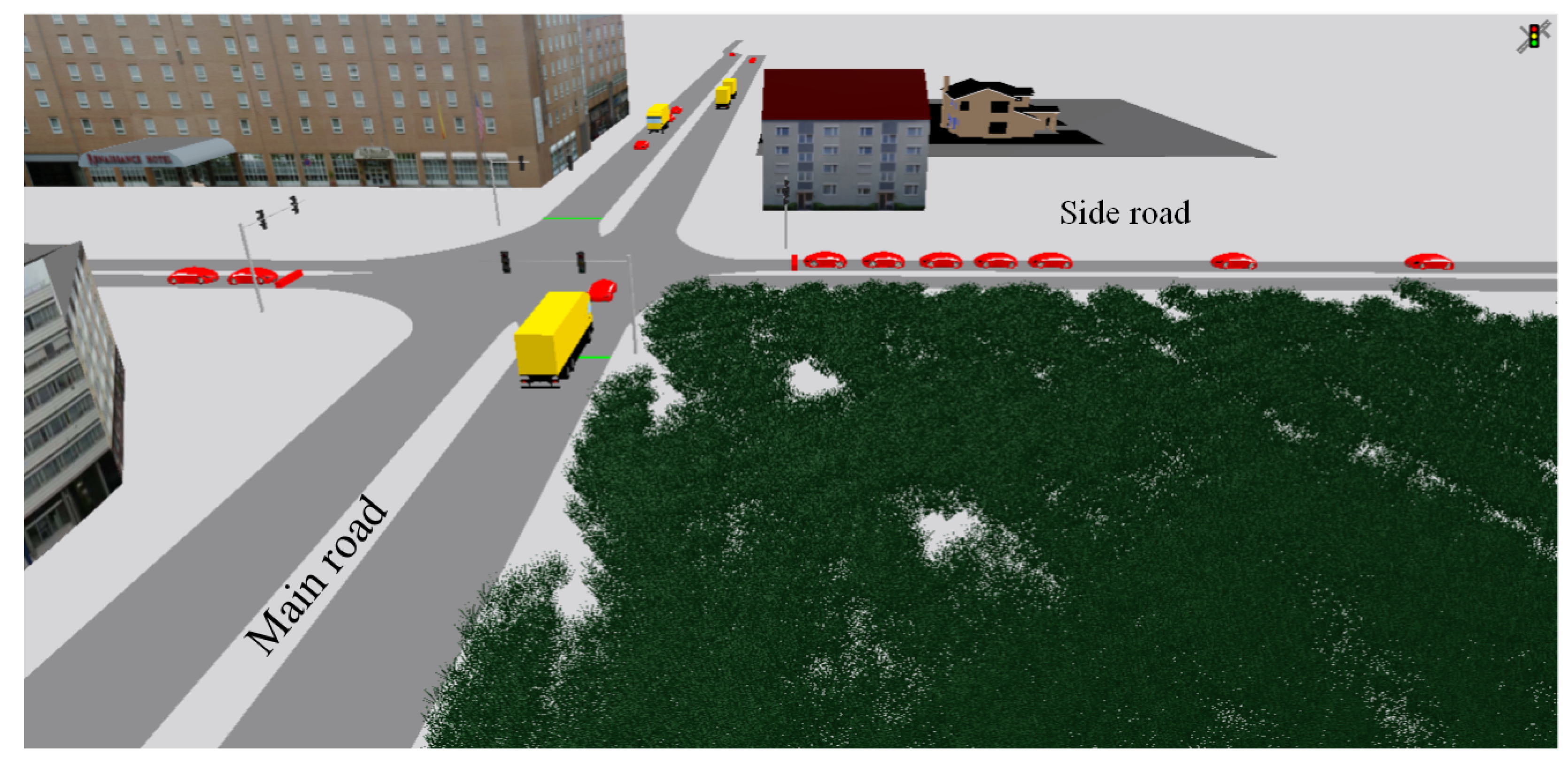
4.1. Formulation of the Basic Intersection

We study a basic intersection with two green time groups, namely, green time group 1 with possibility of green time extension (main road) and green time group 2 without the possibility of a green time extension (side road). Both roads have two single lanes in opposing directions (lanes 1 and 2). The parameters and their reference values used throughout these numerical examples are shown in

Table 1. Reference values of parameters.

${\lambda }_{n,1,1}$ = ${\lambda }_{n,1,2}$ = $0.15$ veh/s (540 veh/h)	${\lambda }_{f,1,1}$ = ${\lambda }_{f,1,2}$ = $0.03$ veh/s (108 veh/h)
${\lambda }_{n,2,1}$ = ${\lambda }_{n,2,2}$ = $0.021$ veh/s (75 veh/h)	${\lambda }_{f,2,1}$ = ${\lambda }_{f,2,2}$ = $0.007$ veh/s (25 veh/h)
$l_n=8$ m	$l_f=18$ m
$v_n=10$ m/s	$v_f=5$ m/s
$t_{r,1}=19$ s	$t_{r,2}=39$ s
$t_{g,1}=31$ s	$t_{g,2}=11$ s

. Furthermore, the green time extension $t_{eg,1}$ was initially set to 10 s. More detail on how we chose these values can be found in Appendix A, but we summarize them here:

• a regular vehicle was assumed to occupy an average length of 8 m (5 m average length plus 3 m as an average buffer length);
• a freight vehicle was assumed to occupy an average length of 18 m (15 m average length plus 3 m as an average buffer length);
• the average speed for a regular vehicle to leave the intersection can be considered as 10 m/s [35];
• based on the results reported in [36], 5 m/s is a good estimation of the average speed for freight vehicles crossing the intersection;
• we have utilized the formulation proposed in [37] to calculate the optimal cycle length (without green extension) and the lengths of the regular red and green periods;
• a green extension interval of 10 s seems a natural choice;
• an illustration of the layout of the basic intersection is depicted in Figure 3.

4.2. Formulation of the Expected Waiting Time and the Optimal Extension Interval

We have two arrival streams (normal and freight vehicles) per lane, leading to eight arrival streams in total. The expected waiting time of a randomly tagged vehicle (irrespective of the lane, green time group or type) in the basic intersection is therefore given by

$$\begin{array}{c}\hfill \mathrm{E}\left[W\right]={\displaystyle \frac{{\sum }_{i,l=1}^2\left({\lambda }_{n,i,l}\mathrm{E}\left[W_{n,i,l}\right]+{\lambda }_{f,i,l}\mathrm{E}\left[W_{f,i,l}\right]\right)}{{\sum }_{i,l=1}^2({\lambda }_{n,i,l}+{\lambda }_{f,i,l})}}.\end{array}$$

(42)

Since the terms in the numerator of Equation (42) all depend on the value of the extension interval, we can find the optimal extension interval resulting in the minimum total expected waiting time. To do that, we approximate $\mathrm{E}\left[W_{n,i,l}\right]$ and $\mathrm{E}\left[W_{f,i,l}\right]$ by the final expressions we obtained for Equations (2) and (3), with X being either {green time group 1} (extension for the main road) or ∅ (no extension for the main road).

4.3. Expected Waiting Times

We first study the mean waiting times of regular and freight vehicles arriving on the main and side road separately and compare them with a pre-timed setting without green time extension ($t_{eg,1}=0$); cf.

Table 2. Expected waiting time of a tagged vehicle.

Expected Waiting Time for a Green Extension Strategy	Expected Waiting Time in the Pre-Timed Setting
$\mathrm{E}\left[W_{n,1}\right]$ = $4.44$ s	$\mathrm{E}\left[W_{n,1}\right]$ = $5.13$ s
$\mathrm{E}\left[W_{f,1}\right]$ = $3.78$ s	$\mathrm{E}\left[W_{f,1}\right]$ = $5.43$ s
$\mathrm{E}\left[W_{n,2}\right]$ = $18.47$ s	$\mathrm{E}\left[W_{n,2}\right]$ = $15.97$ s
$\mathrm{E}\left[W_{f,2}\right]$ = $18.71$ s	$\mathrm{E}\left[W_{f,2}\right]$ = $16.18$ s

(all terms in seconds). Since traffic is assumed to be symmetric in the reference case, waiting times in different lanes for the same vehicle type and the same green time group are equal.

The pattern in the obtained results was expected because the green extension strategy favors the vehicles on the main road over those on the side road. Compared to the pre-timed setting, our approximation confirms that extending green time with an extension interval could result in better performance, since it could overcome the non-homogeneities caused by the stop-and-go events of freight vehicles. Note that the regular vehicles on the main road profit as well. Obviously, the decrease in the expected waiting times of vehicles on the main road comes at the cost of an increase in the average delay of vehicles on the side road. Accordingly, the green extension interval length should balance these advantageous and disadvantageous effects. Before focusing on the optimal extension interval, we first report some sensitivity analysis.

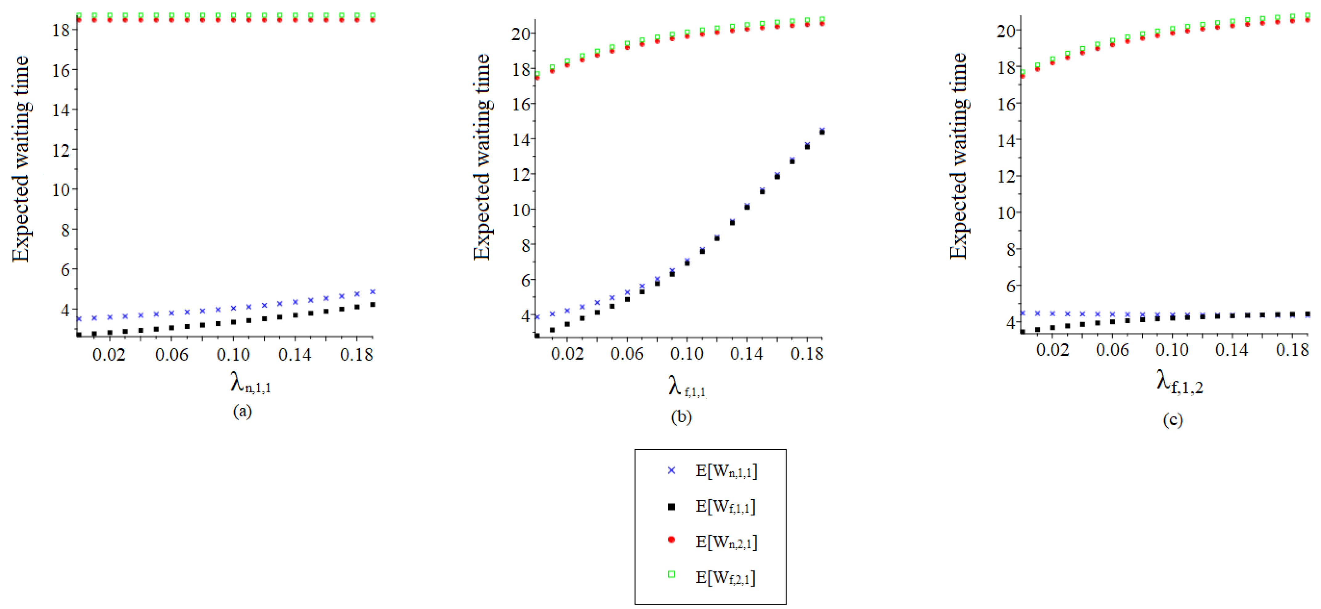
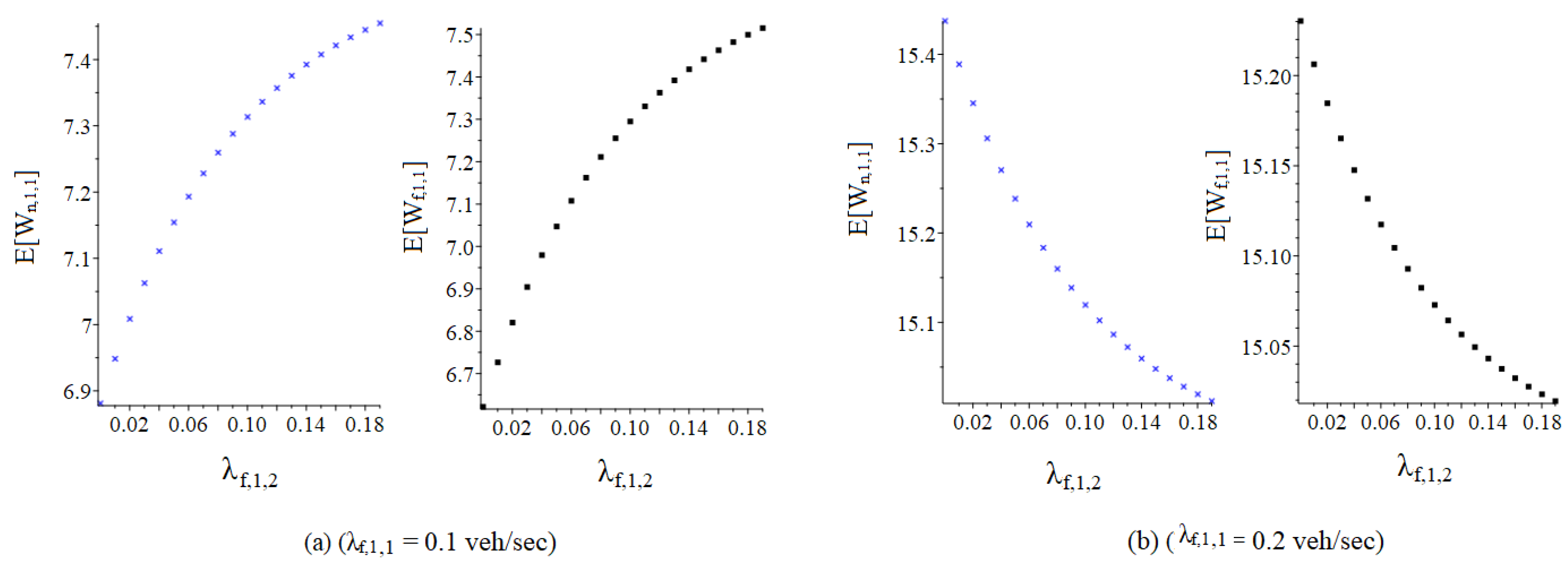
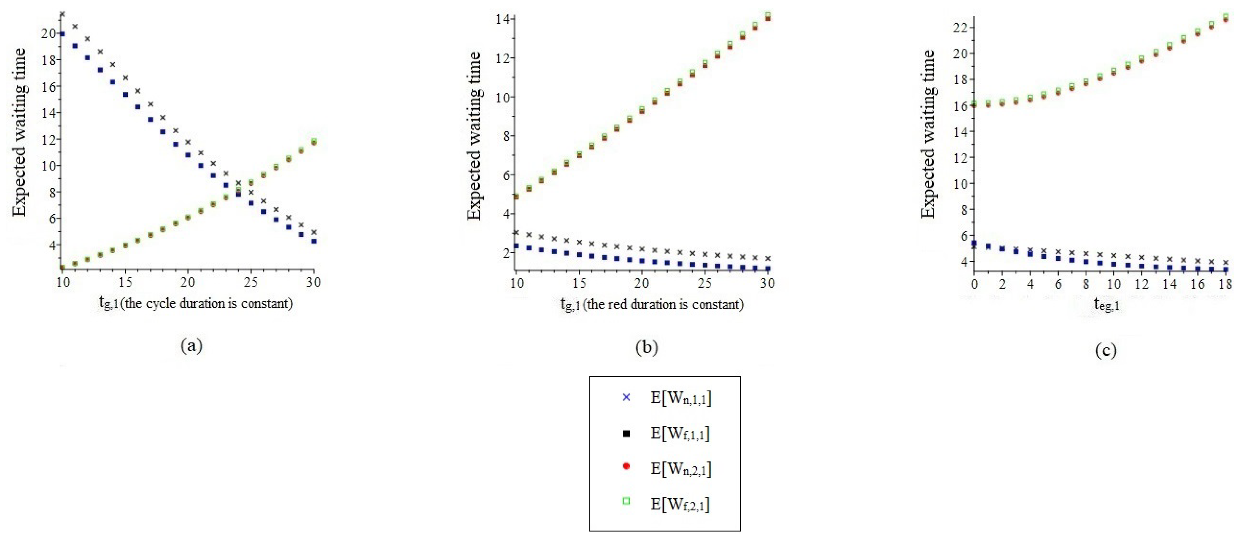
4.4. Sensitivity Analysis of Individual Parameters

In this section, the influences of some of the important parameters on the expected waiting times of regular and freight vehicles are investigated. This study was performed by varying one parameter each time and keeping the others constant and equal to the reference values, as presented in the previous paragraph. Since the situation is then asymmetric, we investigated the mean waiting times of regular and freight vehicles in one particular lane each of the main and side roads (more precisely, lane 1 in all cases).

In order to investigate the influence of the arrival rates of freight and regular vehicles on the main road (in the vehicle’s own or opposite lane) on the expected waiting times for a given type of vehicle in a certain lane, we considered a range of arrival rates for these types of vehicles and approximated the expected waiting times, as shown in Figure 4 (we used Maple software for the calculations and drawing of the figures). All other parameters were as indicated in Table 1.

First, we show the expected waiting times of regular and freight vehicles in lane 1 of the main and side roads as functions of the arrival rate of regular vehicles in lane 1 of the main road in Figure 4a. This figure shows that increasing the arrival rate of regular vehicles on the main road will cause the average waiting time in that lane to become larger. Since regular vehicles are not able to cause an extension interval, we see no influence on the expected waiting time of vehicles on the side road.

Second, we show the impact of the arrival rate of freight vehicles in lane 1 of the main road on the same average waiting times in Figure 4b. The figure shows that increasing the arrival rate of freight vehicles on the main road leads to a longer expected waiting time for both types of vehicles in the same lane on the main road, and for those on the side road. In fact, a higher ${\lambda }_{f,1,1}$, on the one hand, causes the average queue length on the main road to increase, and on the other hand, extends the red time for the side-road vehicles. Furthermore, the probability that a regular vehicle is stuck behind a freight vehicle and consequently leaves the intersection at a lower speed also increases.

Third, Figure 4c highlights the effect of the arrival rate of freight vehicles in the opposite direction (lane 2) of the tagged vehicle on the main road. A higher ${\lambda }_{f,1,2}$ also increases the number of times in which a green extension is triggered. Therefore, the expected waiting times of vehicles on the side road increase. However, the effect on the expected waiting times of regular (freight) vehicles on lane 1 of the main road is not unambiguous and depends on the other parameters, such as the arrival rate ${\lambda }_{f,1,1}$ of freight vehicles in that lane. For low values of ${\lambda }_{f,1,1}$, such as ${\lambda }_{f,1,1}=0.03$ shown in Figure 4c, an increase in ${\lambda }_{f,1,2}$ results in (slightly) lower expected waiting times for the regular vehicles and (slightly) higher expected waiting times for the freight vehicles on the main road. While the obtained result seems counter-intuitive at first glance, one should realize that a higher ${\lambda }_{f,1,2}$ means that the distribution of extension cycles will become dependent on the freight vehicles in the opposite lane. Therefore, the possibility that a freight vehicle arrives on the main road when the extension interval was already applied for the opposite lane increases. Accordingly, a higher expected waiting time results from an increase in ${\lambda }_{f,1,2}$ for low values of ${\lambda }_{f,1,1}$. On the contrary, such extensions can decrease the expected waiting times of regular vehicles by extending relatively more cycles. For a somewhat higher ${\lambda }_{f,1,1}$ (e.g., ${\lambda }_{f,1,1}=0.1$ veh/s), the probability of a freight vehicle waiting in the queue in front of a regular vehicle increases and becomes dominant. As a result, the expected waiting times of regular vehicles and freight vehicles increase with ${\lambda }_{f,1,2}$ in that case, as is shown in Figure 5a. If we increase ${\lambda }_{f,1,1}$ even further (e.g., ${\lambda }_{f,1,1}=0.2$ veh/s in our example), the mentioned dominance gradually fades due to the relatively lower number of regular vehicles in traffic streams, but there are more extended cycles with an increase in ${\lambda }_{f,1,2}$. Furthermore, given the high value of ${\lambda }_{f,1,1}$, the distribution of extension cycles will remain dependent on the freight vehicles on the main road. Both these taken into account, as is shown in Figure 5b; the expected waiting times decrease for both regular vehicles and freight vehicles in such a case.

Based on the above observations and explanations, we conclude that the green extension strategy should be applied with care, since the arrival rate of freight vehicles arriving from a certain direction can either positively or negatively impact the expected waiting times of vehicles arriving from the other directions within the same green time groups. Such a result highlights the importance of using optimal green extension intervals based on the traffic profile.

In order to see the influences of (1) changing the green time period in the case of constant cycle duration, (2) the green time period in the case of constant red time duration and (3) the green time extension on the mean expected waiting times, we show in Figure 6 that:

• with constant cycle duration, the expected mean waiting times of vehicles on the main (side) road decrease (increases) drastically with increasing green time for the main road (Figure 6a);
• with constant red time for the main road, the mean expected waiting times of vehicles on the main road decrease mildly, while the mean expected waiting times of vehicles on the side road increase drastically with increasing green times for the main road (Figure 6b);
• a higher green time extension, on the one hand, has a varying positive effect on the expected waiting times of vehicles on the main road, and on the other hand, has a varying negative effect on the expected waiting times of vehicles on the side road (Figure 6c).

From the above-enumerated results, the latter argument (Figure 6c) also highlights the need for determining an optimal $t_{eg,1}$.

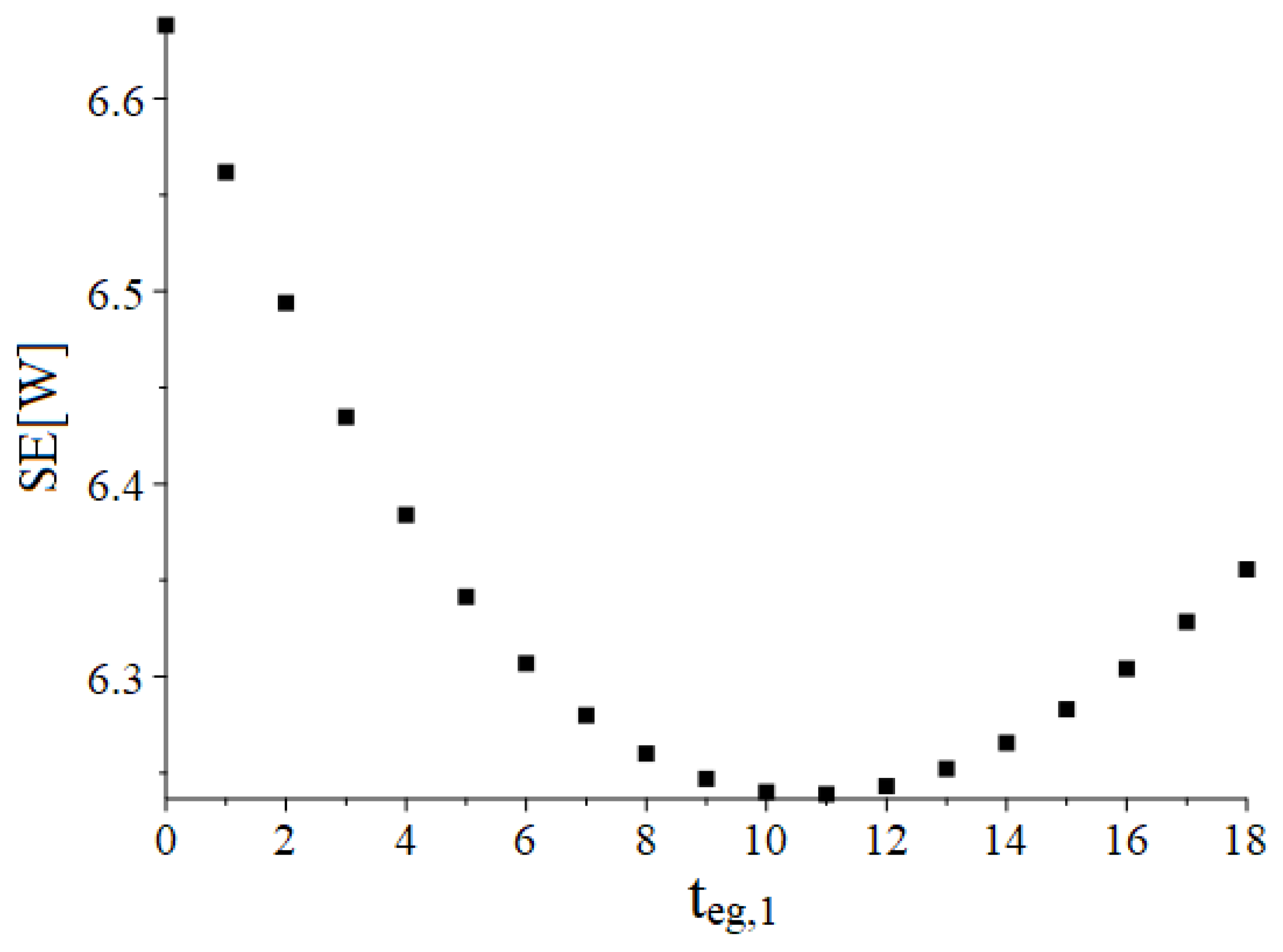
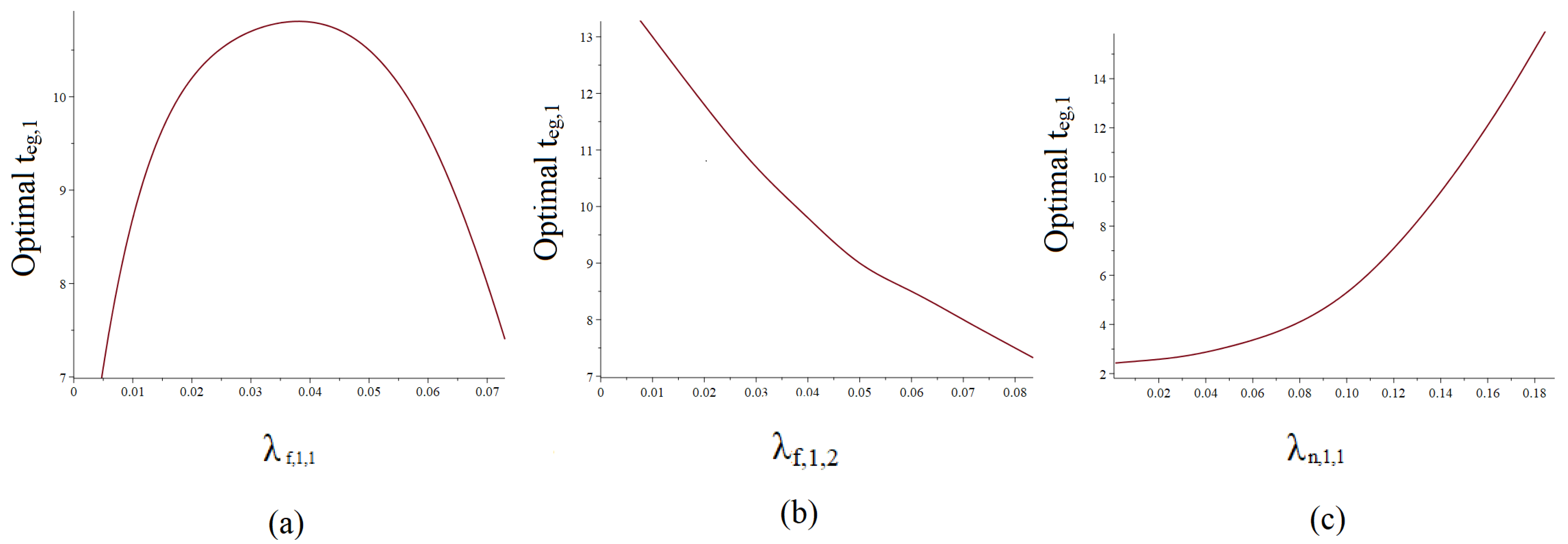
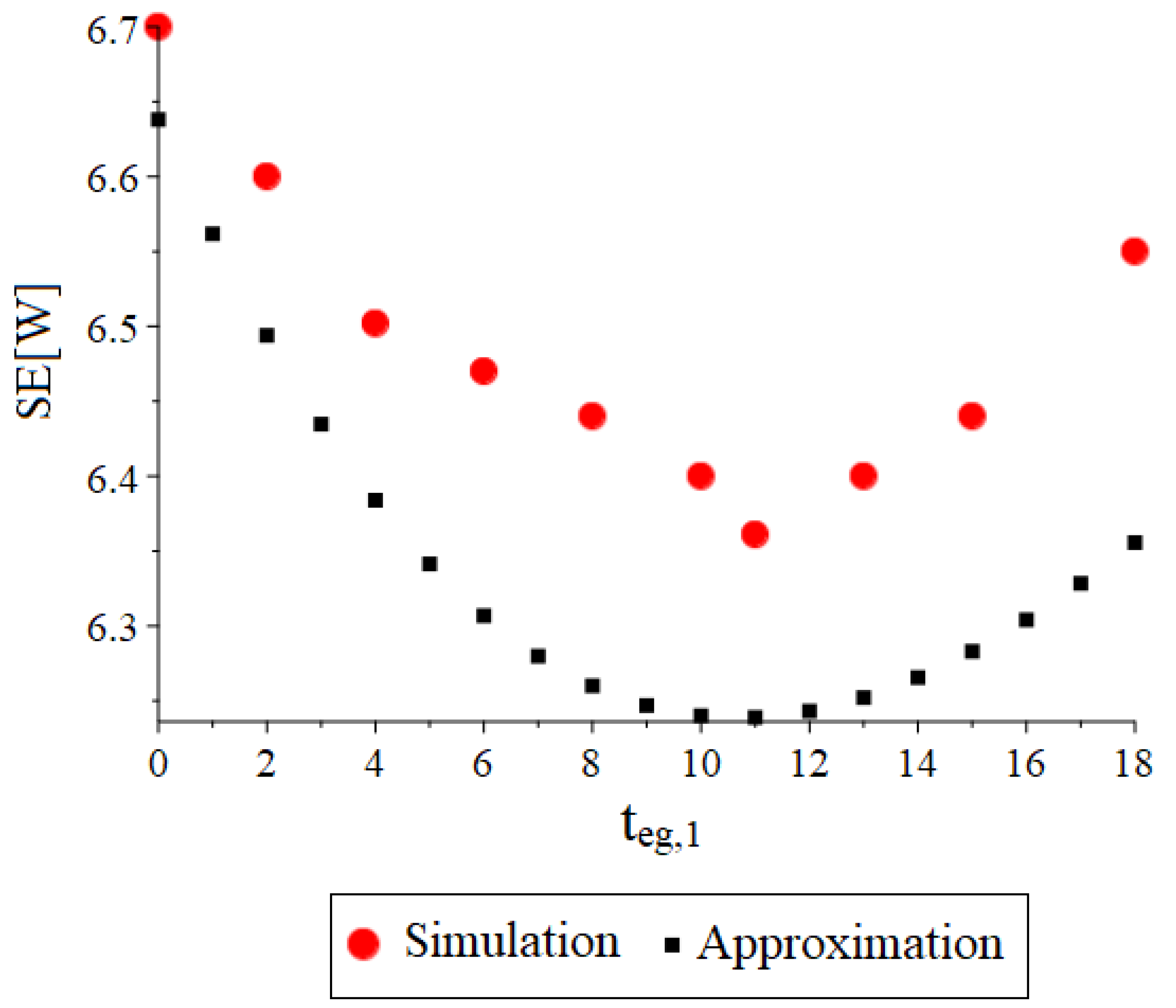
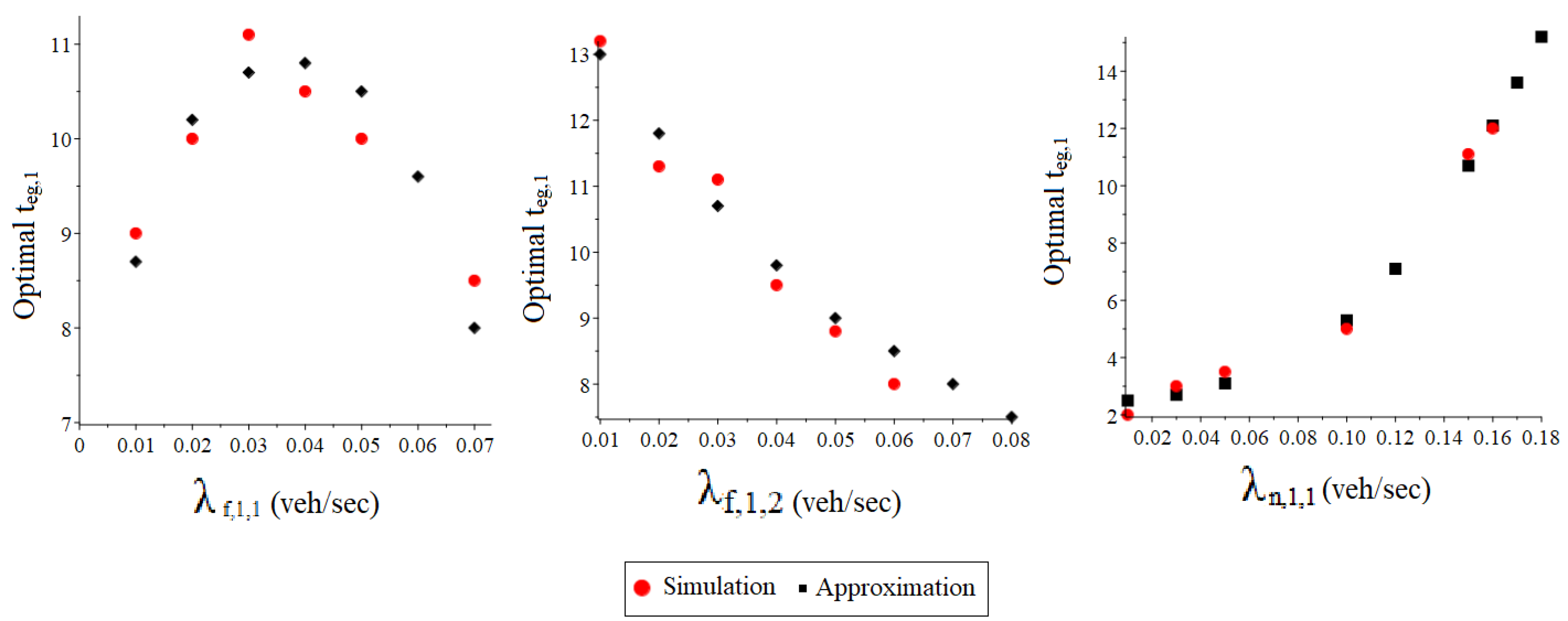
4.5. Optimal Extension Interval

To find the optimal length of the extension interval, we use the proposed formulation to show how the expected waiting time of an arbitrary vehicle (i.e., waiting times averaged over all vehicles in all green time groups) changes with $t_{eg,1}$. The results of this approximation with the base case summarized in Section 4.1 are presented in Figure 7. This figure shows that there is a clear optimal value for the green time extension interval.

Next, we investigate the sensitivity of the optimal mean expected waiting time to the change of (1) the arrival rate of freight vehicles on the main road (${\lambda }_{f,1,1}={\lambda }_{f,1,2}$), (2) the arrival rate of freight vehicles on the main road in the opposite direction of the tagged vehicle (${\lambda }_{f,1,2}$ while ${\lambda }_{f,1,1}$ is kept constant) and (3) the arrival rate of regular vehicles on the main road (${\lambda }_{n,1,1}={\lambda }_{n,1,2}$) with the results shown in Figure 8. Based on Figure 8a, we conclude that the optimal $t_{eg,1}$ increases with the (symmetric) arrival rate of freight vehicles up to some point ($0.04$ for our example), after which it decreases again. Based on Figure 8b, if the rate of freight vehicles on the main road in one of the lanes increases, the optimal $t_{eg,1}$ decreases. Finally, as is shown in Figure 8c, if the arrival rate of regular vehicles on the main road increases, the optimal $t_{eg,1}$ increases as well. This figure confirms that there is a need to modify the length of the extension interval in accordance with (expected) changes in traffic conditions at an intersection.

4.6. Validation of the Optimal Extension Interval

In our analysis, we imposed a critical assumption that no vehicles stay behind at the end of a green time in our analysis, and we adopted a fluid-flow approximation in the case that a vehicle arrives during a green time to avoid the concomitant complexities in the analysis. Now, to validate our analysis in relatively light traffic (that is the case of our interest) against the effects of these assumptions, the VISSIM micro-simulator is adopted here to generate traffic data as realistically as possible. Accordingly, we developed an internal script representing the basic intersection in the VISSIM simulation environment (see the layout in Figure 3). (The reader can find the applied script at https://github.com/SaraSasaninejad/Green-Extension-VISSIM/blob/main/1.py.) Next, we carried out several series of three-hour simulations under dynamic loading with considering different $t_{eg,1}$s to (1) compare the expected waiting times calculated from our approximation with the expected waiting times resulting from VISSIM and (2) compare the associated optimal extension intervals.

Figure 9 shows the results of this comparison for the basic model (see Table 1 for the reference values). According to this Figure, simulations result in higher expected waiting times, due to the consideration of all micro parameters affecting the flow of traffic. For example, our analysis did not consider the acceleration/deceleration law and shockwave boundaries. Furthermore, given the possibility of overflow queues even for light traffic, we can see fluctuations in the expected waiting times resulting from simulations. However, it is interesting to see that both our analysis and the simulations resulted in the same pattern of the mean waiting time as a function of the green extension time, and that they gave almost the same optimal extension interval that is $10.7$ s for our approximation and 11 s for VISSIM.

We also carried out several runs of simulations to mimic the parameters used in Figure 8 and compare the resulting optimal $t_{eg,1}$ with the ones in that figure. Figure 10 provides this comparison which in turn confirms that our analysis results in the optimal $t_{eg,1}$, which is satisfactorily close to that of simulations under a plethora of conditions.

With all this taken into account, we can conclude that this analysis, on the one hand, provides a good approximation of the expected waiting times, and on the other hand, results in accurate optimal extension interval values. Accordingly, it can be efficiently used to calculate the associated optimal extension interval in a dynamic environment.

5. Conclusions

In this study, a novel stochastic model suitable for estimating the impact of a green time extension strategy for signalized intersections has been developed and analyzed. The model does not require much computational power and specialized expertise, making it an interesting tool to perform a preliminary investigation on the impact of a green extension strategy. The analysis was validated by comparing the obtained results with those of simulations.

The performance measures used were the expected waiting times of different vehicle streams. By comparing the expected waiting times in a reference intersection, with and without the use of a green time extension strategy, we evaluated the effect of the extension interval length. In this respect, we see that using extension intervals could lead to both

• decreases in the expected waiting times of regular and freight vehicles in green time groups capable of extending green time;
• an increase in the mean expected waiting time of vehicles in other green time groups.

Given such contradictory effects, an analysis incorporating traffic conditions in all green time groups on the one hand, and the length of the extension interval on the other, seems inevitable in order to obtain optimal performance. Accordingly, we have first employed the proposed analysis to calculate the expected waiting time to present a sensitivity analysis on the arrival rates of different vehicles, the duration of green time, cycle length, etc. Second, we have embedded this performance measure in an algorithm, resulting in the optimal green extension interval. Given further the validation process, we observed that

• the proposed approximation can appropriately capture the effects of different traffic parameters to estimate expected waiting times;
• the accuracy of the approximation of the expected waiting time is acceptable;
• the optimal extension interval resulting from our analysis coincides with that from micro simulations.

To highlight the implications of this analysis, we refer to increasing progress in the advanced intersection controllers that, on the one hand, consider a priority for some special types of vehicles, and on the other hand, aim to increase the overall traffic efficiency. One of the main challenges in such systems is the high computational burden resulting from the analysis of a high volume of data in a simulation environment. Our results show, however, that the proposed analysis is a good compromise between accuracy and computational efficiency.

This paper opens the following research directions:

• Extending the current analysis to more general arrival patterns to address traffic characteristics in a network of intersections. In this regard, the incorporation of batch arrivals (platoons) consisting of different vehicles is needed, similarly to the model presented in [38]. A second extension in this regard is multiple lanes per input–output pair of the intersection where vehicles can overtake each other.
• A proper queuing analysis (including overspill between cycles) is also interesting, although it could be a difficult task. In this case (an expected value of), the overflow queue should also be incorporated in the current analysis. To this end, the analysis presented in some related papers (e.g., [39,40]) can be helpful.
• Integrating this analysis in an advanced intelligent intersection controller to quantify its implications.

References

1. Holguín-Veras, J.; Leal, J.A.; Sánchez-Diaz, I.; Browne, M.; Wojtowicz, J. State of the art and practice of urban freight management: Part I: Infrastructure, vehicle-related, and traffic operations. Transp. Res. Part A Policy Pract. 2018, 137, 360–382. [Google Scholar] [CrossRef]
2. Lafkihi, M.; Pan, S.; Ballot, E. Freight transportation service procurement: A literature review and future research opportunities in omnichannel E-commerce. Transp. Res. Part E Logist. Transp. Rev. 2019, 125, 348–365. [Google Scholar] [CrossRef]
3. Xia, X.; Ma, X.; Wang, J. Control method for signalized intersection with integrated waiting area. Appl. Sci. 2019, 9, 968. [Google Scholar] [CrossRef]
4. Blokpoel, R.; Hausberger, S.; Krajzewicz, D. Emission optimised control and speed limit for isolated intersections. IET Intell. Transp. Syst. 2017, 11, 174–181. [Google Scholar] [CrossRef]
5. Moradi, H.; Sasaninejad, S.; Wittevrongel, S.; Walraevens, J. Proposal of an integrated platoon-based Round-Robin algorithm with priorities for intersections with mixed traffic flows. IET Intell. Transp. Syst. 2021, 15, 1106–1118. [Google Scholar] [CrossRef]
6. Wang, K.; Zhu, F. A real-time BRT signal priority approach through two-stage green extension. In Proceedings of the 2012 9th IEEE International Conference on Networking, Sensing and Control, Beijing, China, 11–14 April 2012; pp. 7–11. [Google Scholar]
7. Niu, X.; Cao, H.; Zhao, Z.; Zhang, T. An optimized signal timing of Transit Signal Priority on early green control strategy. In Proceedings of the 2011 International Conference on Transportation, Mechanical, and Electrical Engineering (TMEE), Changchun, China, 16–18 December 2011; pp. 2552–2555. [Google Scholar]
8. Lee, J.; Shalaby, A.; Greenough, J.; Bowie, M.; Hung, S. Advanced transit signal priority control with online microsimulation-based transit prediction model. Transp. Res. Rec. 2005, 1925, 185–194. [Google Scholar] [CrossRef]
9. Truong, L.T.; Currie, G.; Wallace, M.; De Gruyter, C. Analytical approach to estimate delay reduction associated with bus priority measures. IEEE Intell. Transp. Syst. Mag. 2017, 9, 91–101. [Google Scholar] [CrossRef]
10. Mei, Z.; Tan, Z.; Zhang, W.; Wang, D. Simulation analysis of traffic signal control and transit signal priority strategies under Arterial Coordination Conditions. Simulation 2019, 95, 51–64. [Google Scholar] [CrossRef]
11. Abdy, Z.R.; Hellinga, B.R. Analytical method for estimating the impact of transit signal priority on vehicle delay. J. Transp. Eng. 2011, 137, 589–600. [Google Scholar] [CrossRef]
12. Hongchao, L.; Zhang, J.; Cheng, D. Analytical approach to evaluating transit signal priority. J. Transp. Syst. Eng. Inf. Technol. 2008, 8, 48–57. [Google Scholar]
13. Lin, Y.; Yang, X.; Zou, N.; Franz, M. Transit signal priority control at signalized intersections: A comprehensive review. Transp. Lett. 2015, 7, 168–180. [Google Scholar] [CrossRef]
14. Heidemann, D. Queue length and delay distributions at traffic signals. Transp. Res. Part B Methodol. 1994, 28, 377–389. [Google Scholar] [CrossRef]
15. Viti, F.; Van Zuylen, H.J. A probabilistic model for traffic at actuated control signals. Transp. Res. Part C Emerg. Technol. 2010, 18, 299–310. [Google Scholar] [CrossRef]
16. Viti, F.; Van Zuylen, H.J. Probabilistic models for queues at fixed control signals. Transp. Res. Part B Methodol. 2010, 44, 120–135. [Google Scholar] [CrossRef]
17. Estrada, M.; Mensión, J.; Aymamí, J.M.; Torres, L. Bus control strategies in corridors with signalized intersections. Transp. Res. Part C Emerg. Technol. 2016, 71, 500–520. [Google Scholar] [CrossRef]
18. Gómez-Marín, C.G.; Arango-Serna, M.D.; Serna-Urán, C.A.; Zapata-Córtes, J.A. Microsimulation as an optimization tool for urban goods distribution: A review. In Proceedings of the MOVICI-MOYCOT 2018: Joint Conference for Urban Mobility in the Smart City, IET, Medellin, Colombia, 18–20 April 2018; pp. 1–8. [Google Scholar]
19. Gomez-Marin, C.G.; Serna-Uran, C.A.; Arango-Serna, M.D.; Comi, A. Microsimulation-based collaboration model for urban freight distribution. IEEE Access 2020, 8, 182853–182867. [Google Scholar] [CrossRef]
20. Ye, B.L.; Wu, W.; Ruan, K.; Li, L.; Chen, T.; Gao, H.; Chen, Y. A survey of model predictive control methods for traffic signal control. IEEE/CAA J. Autom. Sin. 2019, 6, 623–640. [Google Scholar] [CrossRef]
21. Li, P.; Wang, T.; Kang, Y.; Li, K.; Zhao, Y.B. Event-based model predictive control for nonlinear systems with dynamic disturbance. Automatica 2022, 145, 110533. [Google Scholar] [CrossRef]
22. Jafari, S.; Shahbazi, Z.; Byun, Y.C. Improving the Performance of Single-Intersection Urban Traffic Networks Based on a Model Predictive Controller. Sustainability 2021, 13, 5630. [Google Scholar] [CrossRef]
23. Moradi, H.; Sasaninejad, S.; Wittevrongel, S.; Walraevens, J. The contribution of connected vehicles to network traffic control: A hierarchical approach. Transp. Res. Part C Emerg. Technol. 2022, 139, 103644. [Google Scholar] [CrossRef]
24. Zhang, T.; Song, W.; Fu, M.; Yang, Y.; Wang, M. Vehicle motion prediction at intersections based on the turning intention and prior trajectories model. IEEE/CAA J. Autom. Sin. 2021, 8, 1657–1666. [Google Scholar] [CrossRef]
25. Ma, Y.; Sun, C.; Chen, J.; Cao, D.; Xiong, L. Verification and validation methods for decision-making and planning of automated vehicles: A review. IEEE Trans. Intell. Veh. 2022, 7, 480–498. [Google Scholar] [CrossRef]
26. Qi, L.; Zhou, M.; Luan, W. Impact of driving behavior on traffic delay at a congested signalized intersection. IEEE Trans. Intell. Transp. Syst. 2016, 18, 1882–1893. [Google Scholar] [CrossRef]
27. Farid, Y.Z.; Christofa, E.; Collura, J. An analytical model to conduct a person-based evaluation of transit preferential treatments on signalized arterials. Transp. Res. Part C Emerg. Technol. 2018, 90, 411–432. [Google Scholar] [CrossRef]
28. Moradi, H.; Sasaninejad, S.; Wittevrongel, S.; Walraevens, J. Dynamically estimating saturation flow rate at signalized intersections: A data-driven technique. Transp. Plan. Technol. 2023; accepted. [Google Scholar] [CrossRef]
29. Sunkari, S.R.; Beasley, P.S.; Urbanik, T.; Fambro, D.B. Model to evaluate the impacts of bus priority on signalized intersections. Transp. Res. Rec. 1995, 15, 117–123. [Google Scholar]
30. Highway Capacity Manual; Special Report 209; National Research Council: Washington, DC, USA, 1985.
31. Jacobson, J.; Sheffi, Y. Analytical model of traffic delays under bus signal preemption: Theory and application. Transp. Res. Part B Methodol. 1981, 15, 127–138. [Google Scholar] [CrossRef]
32. Lin, W.H. Quantifying delay reduction to buses with signal priority treatment in mixed-mode operation. Transp. Res. Rec. 2002, 1811, 100–106. [Google Scholar] [CrossRef]
33. Walraevens, J.; Maertens, T.; Wittevrongel, S. Extensions of green periods for freight vehicles at signalized intersections: A stochastic analysis. In Proceedings of the 13th International Conference on Queueing Theory and Network Applications (QTNA2018), Tsukuba City, Japan, 25–27 July 2018; pp. 69–73. [Google Scholar]
34. van Leeuwaarden, J.S. Delay analysis for the fixed-cycle traffic-light queue. Transp. Sci. 2006, 40, 189–199. [Google Scholar] [CrossRef]
35. Rouffaert, A.; van ’t Hof, M.; Poelmans, W. Veilige wegen en kruispunten; Agentschap Wegen en Verkeer: Brussels, Belgium, 2009. [Google Scholar]
36. Yang, G.; Xu, H.; Wang, Z.; Tian, Z. Truck acceleration behavior study and acceleration lane length recommendations for metered on-ramps. Int. J. Transp. Sci. Technol. 2016, 5, 93–102. [Google Scholar] [CrossRef]
37. Wolput, B.; Christofa, E.; Tampère, C.M. Optimal cycle-length formulas for intersections with or without transit signal priority. Transp. Res. Rec. 2016, 2558, 78–91. [Google Scholar] [CrossRef]
38. Pang, G.; Whitt, W. Infinite-server queues with batch arrivals and dependent service times. Probab. Eng. Inf. Sci. 2012, 26, 197–220. [Google Scholar] [CrossRef]
39. Liu, H.X.; Wu, X.; Ma, W.; Hu, H. Real-time queue length estimation for congested signalized intersections. Transp. Res. Part C Emerg. Technol. 2009, 17, 412–427. [Google Scholar] [CrossRef]
40. Comert, G.; Cetin, M. Queue length estimation from probe vehicle location and the impacts of sample size. Eur. J. Oper. Res. 2009, 197, 196–202. [Google Scholar] [CrossRef]
Figure 1. Different cases of I f .
Mathematics 11 00721 g001
Figure 2. Examples of different scenarios for the dissolution of the queue during the green time of an extended cycle when no freight vehicle has arrived in the corresponding red time.
Mathematics 11 00721 g002
Figure 3. An illustration of the layout used for the basic intersection.
Mathematics 11 00721 g003
Figure 4. Expected waiting times of vehicles in lanes 1 as functions of (a) arrival rates of regular vehicles on the main road, (b) freight vehicles on the main road and (c) freight vehicles on the main road from the opposite direction.
Mathematics 11 00721 g004
Figure 5. Expected waiting times of vehicles in a lane on the main road as functions of the arrival rate of freight vehicles in the opposite lane.
Mathematics 11 00721 g005
Figure 6. Expected waiting times as functions of (a) green time when the cycle time is constant, (b) of green time when the red time is constant and (c) of green extension time.
Mathematics 11 00721 g006
Figure 7. Expected waiting time as a function of t e g , 1 .
Mathematics 11 00721 g007
Figure 8. Sensitivity of optimal t e g , 1 to the arrival rates of (a) freight vehicles on the main road, (b) freight vehicles in one lane of the main road, and (c) regular vehicles.
Mathematics 11 00721 g008
Figure 9. Expected waiting time as a function of t e g , 1 according to VISSIM.
Mathematics 11 00721 g009
Figure 10. Comparing the optimal t e g , 1 obtained by our analysis with the results of simulations.
Mathematics 11 00721 g010