
Bisecting for Selecting: Using a Laplacian Eigenmaps Clustering Approach to Create the New European Football Super League


Abstract
1. Introduction
2. Materials and Methods
2.1. Data Acquisition
2.2. Data Analysis Strategy
2.3. Initial Analysis
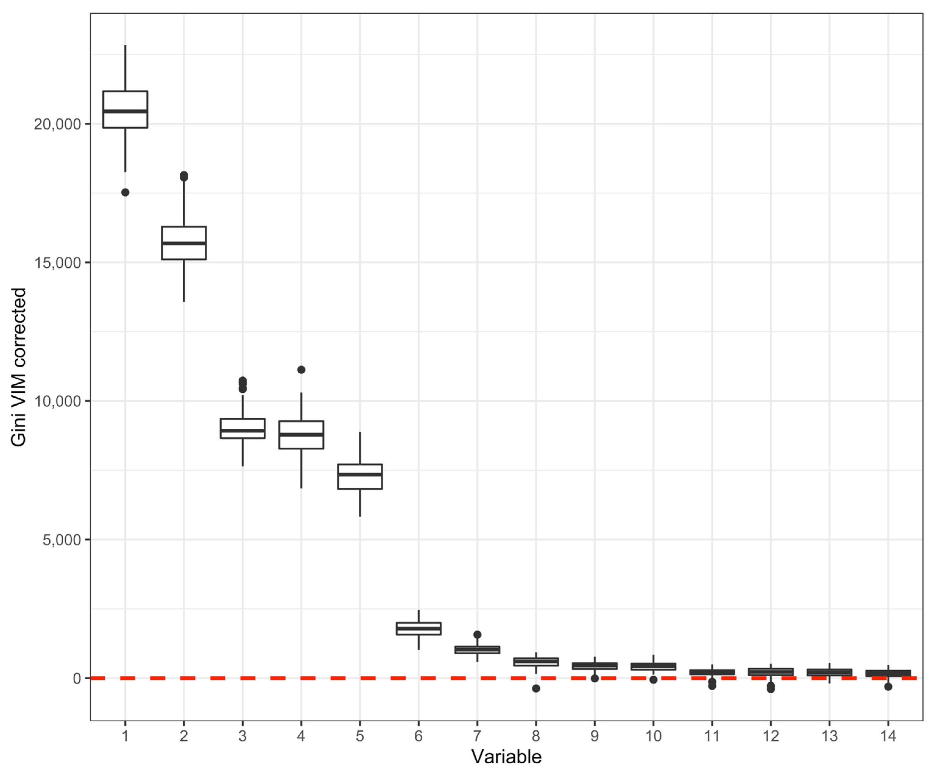
2.4. Exploratory Random Forest Analysis
2.5. Laplacian Eigenmaps
2.6. Natural Clustering Approach
3. Results
3.1. Descriptive Statistics
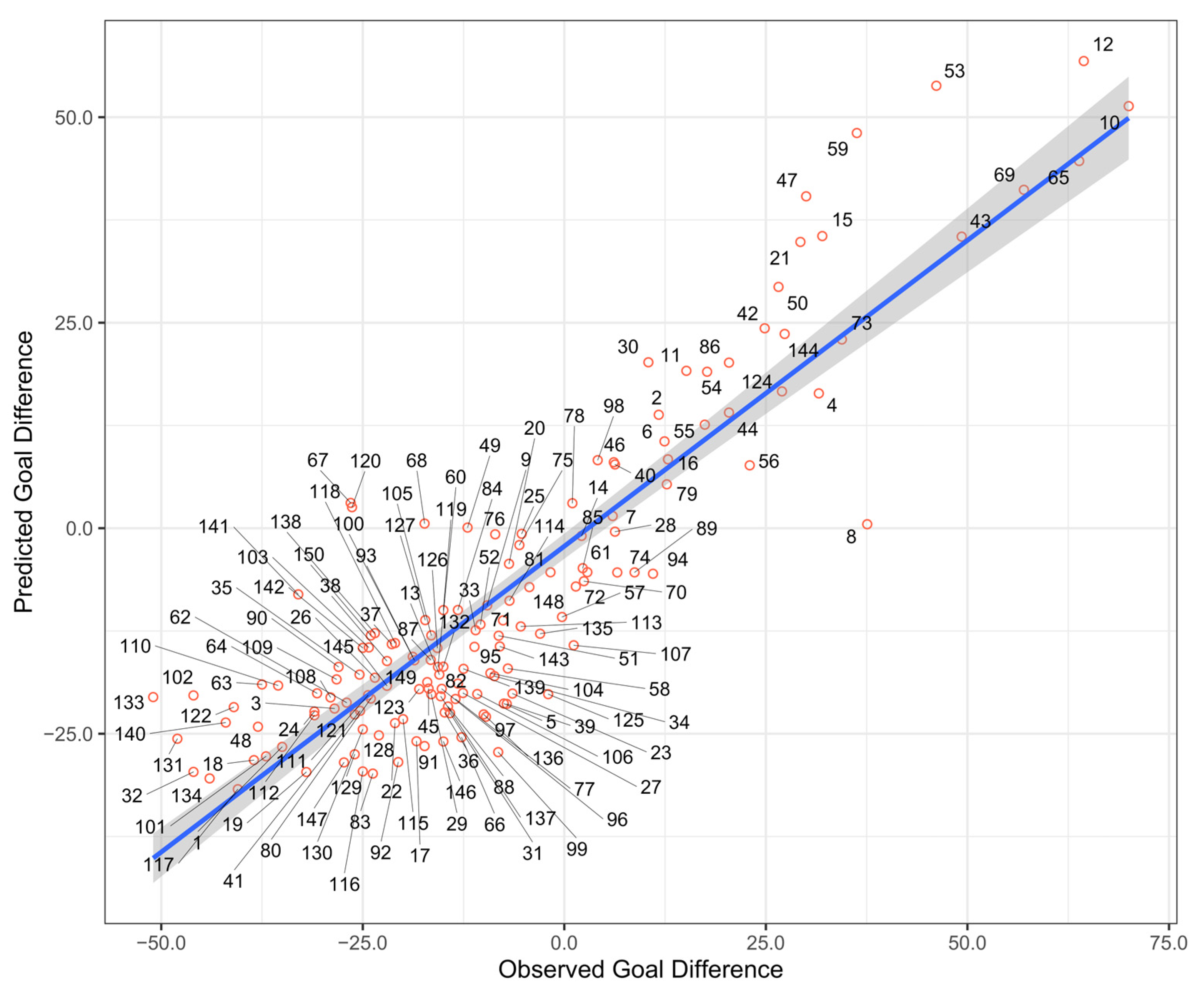
3.2. Random Forest Analysis Results
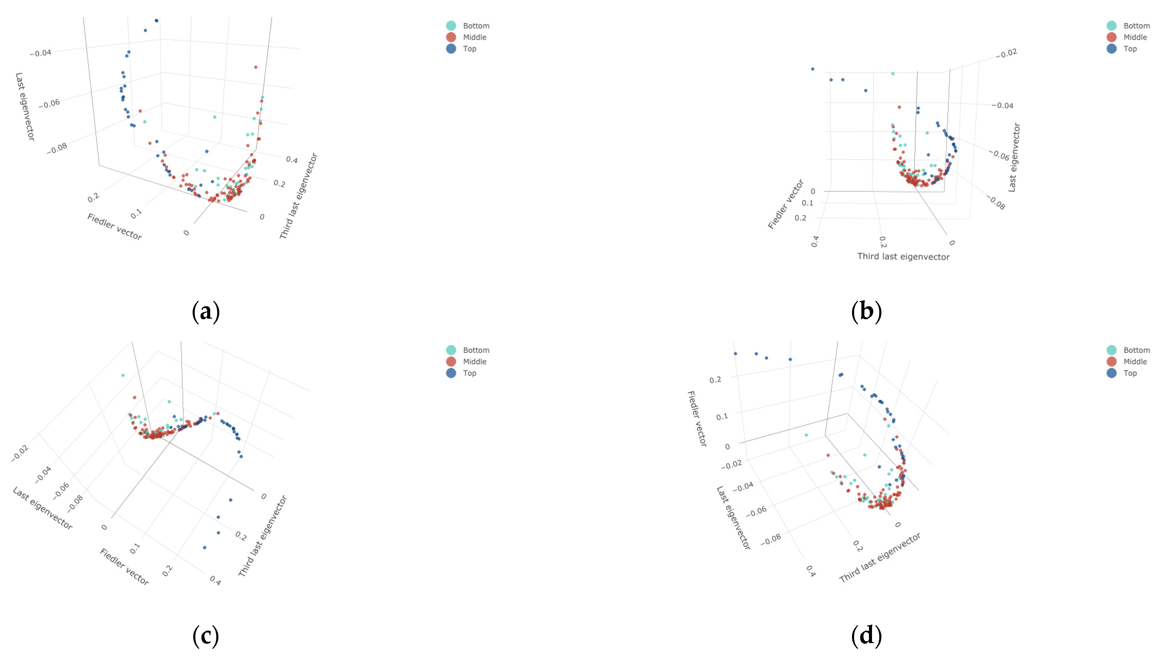
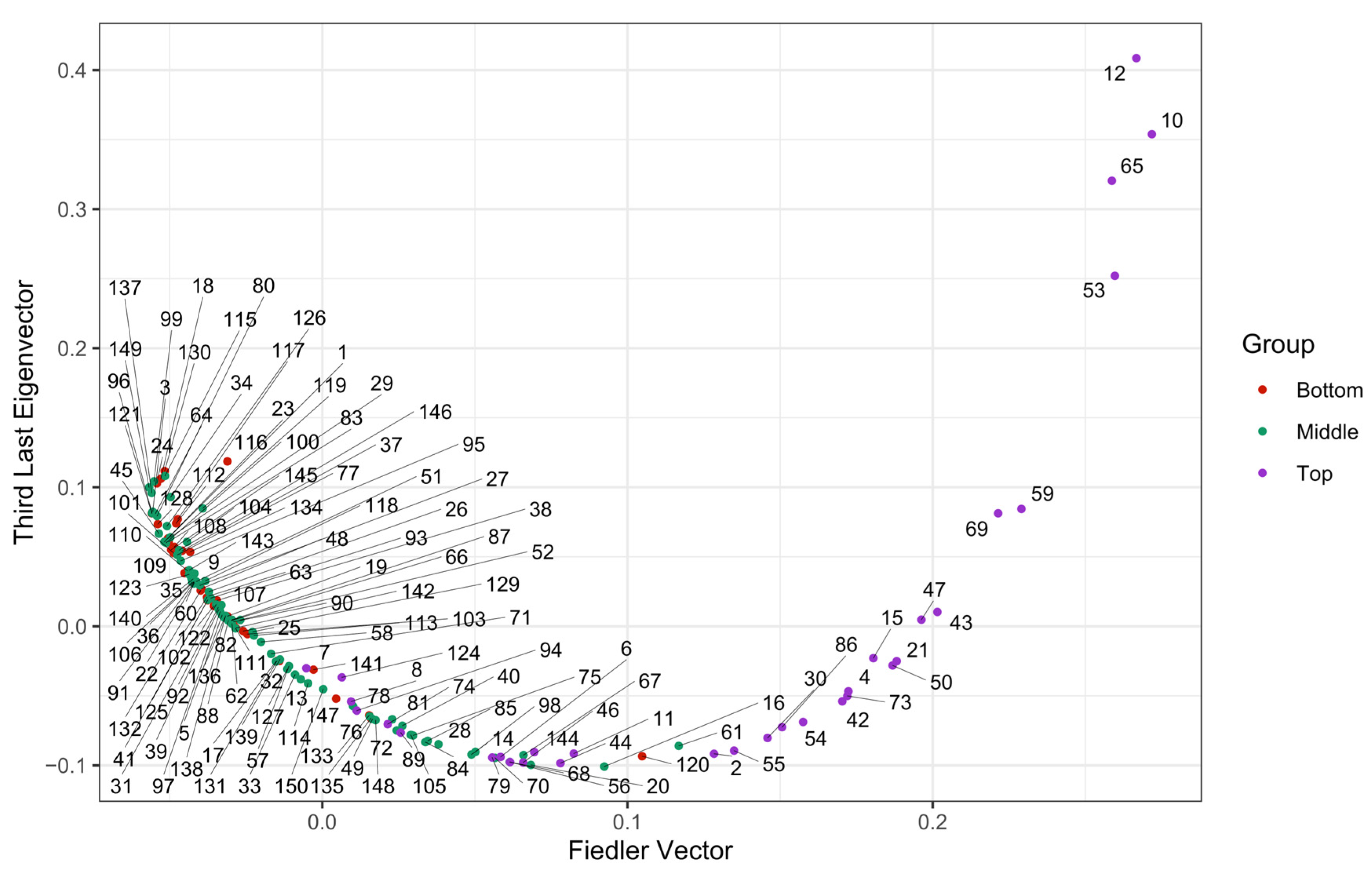
3.3. Laplacian Eigenmap Results
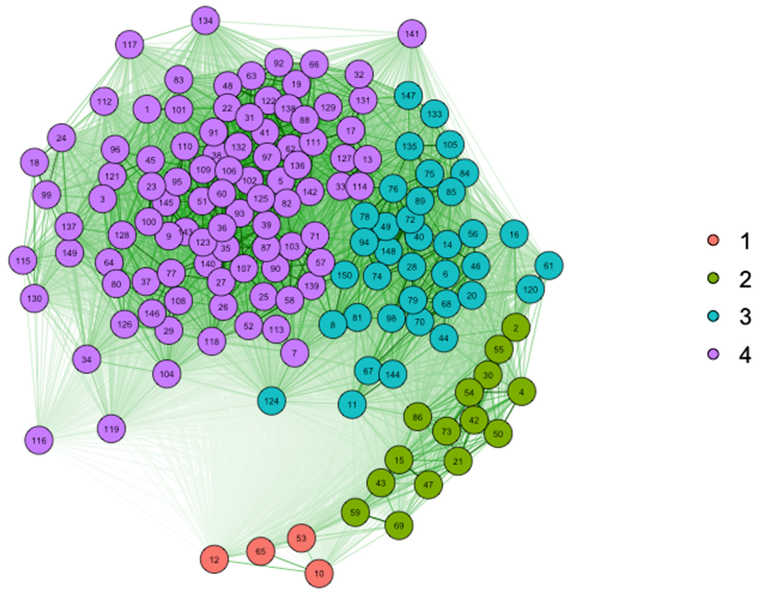
3.4. Natural Clustering Results
4. Discussion
5. Conclusions
Author Contributions
Funding
Data Availability Statement
Conflicts of Interest
Appendix A
| Team_ID | Team | Tournament | Team_ID | Team | Tournament |
| 1 | AC Ajaccio | Ligue 1 | 76 | Sassuolo | Serie A |
| 2 | AC Milan | Serie A | 77 | SC Bastia | Ligue 1 |
| 3 | Almeria | La Liga | 78 | Schalke 04 | Bundesliga |
| 4 | Arsenal | Premier League | 79 | Sevilla | La Liga |
| 5 | Aston Villa | Premier League | 80 | Sochaux | Ligue 1 |
| 6 | Atalanta | Serie A | 81 | Southampton | Premier League |
| 7 | Athletic Bilbao | La Liga | 82 | Stoke | Premier League |
| 8 | Atletico Madrid | La Liga | 83 | Sunderland | Premier League |
| 9 | Augsburg | Bundesliga | 84 | Swansea | Premier League |
| 10 | Barcelona | La Liga | 85 | Torino | Serie A |
| 11 | Bayer Leverkusen | Bundesliga | 86 | Tottenham | Premier League |
| 12 | Bayern Munich | Bundesliga | 87 | Toulouse | Ligue 1 |
| 13 | Bologna | Serie A | 88 | Udinese | Serie A |
| 14 | Bordeaux | Ligue 1 | 89 | Valencia | La Liga |
| 15 | Borussia Dortmund | Bundesliga | 90 | Valenciennes | Ligue 1 |
| 16 | Borussia M.Gladbach | Bundesliga | 91 | Valladolid | La Liga |
| 17 | Cagliari | Serie A | 92 | Verona | Serie A |
| 18 | Cardiff | Premier League | 93 | VfB Stuttgart | Bundesliga |
| 19 | Catania | Serie A | 94 | Villarreal | La Liga |
| 20 | Celta Vigo | La Liga | 95 | Werder Bremen | Bundesliga |
| 21 | Chelsea | Premier League | 96 | West Bromwich Albion | Premier League |
| 22 | Chievo | Serie A | 97 | West Ham | Premier League |
| 23 | Crystal Palace | Premier League | 98 | Wolfsburg | Bundesliga |
| 24 | Eintracht Braunschweig | Bundesliga | 99 | Burnley | Premier League |
| 25 | Eintracht Frankfurt | Bundesliga | 100 | Caen | Ligue 1 |
| 26 | Elche | La Liga | 101 | Cesena | Serie A |
| 27 | Espanyol | La Liga | 102 | Cordoba | La Liga |
| 28 | Everton | Premier League | 103 | Deportivo La Coruna | La Liga |
| 29 | Evian Thonon Gaillard | Ligue 1 | 104 | Eibar | La Liga |
| 30 | Fiorentina | Serie A | 105 | Empoli | Serie A |
| 31 | Freiburg | Bundesliga | 106 | FC Koln | Bundesliga |
| 32 | Fulham | Premier League | 107 | Leicester | Premier League |
| 33 | Genoa | Serie A | 108 | Lens | Ligue 1 |
| 34 | Getafe | La Liga | 109 | Metz | Ligue 1 |
| 35 | Granada | La Liga | 110 | Paderborn | Bundesliga |
| 36 | Guingamp | Ligue 1 | 111 | Palermo | Serie A |
| 37 | Hamburger SV | Bundesliga | 112 | Queens Park Rangers | Premier League |
| 38 | Hannover 96 | Bundesliga | 113 | Angers | Ligue 1 |
| 39 | Hertha Berlin | Bundesliga | 114 | Bournemouth | Premier League |
| 40 | Hoffenheim | Bundesliga | 115 | Carpi | Serie A |
| 41 | Hull | Premier League | 116 | Darmstadt | Bundesliga |
| 42 | Inter Milan | Serie A | 117 | Frosinone | Serie A |
| 43 | Juventus | Serie A | 118 | GFC Ajaccio | Ligue 1 |
| 44 | Lazio | Serie A | 119 | Ingolstadt | Bundesliga |
| 45 | Levante | La Liga | 120 | Las Palmas | La Liga |
| 46 | Lille | Ligue 1 | 121 | Sporting Gijon | La Liga |
| 47 | Liverpool | Premier League | 122 | Troyes | Ligue 1 |
| 48 | Livorno | Serie A | 123 | Watford | Premier League |
| 49 | Lorient | Ligue 1 | 124 | RasenBallsport Leipzig | Bundesliga |
| 50 | Lyon | Ligue 1 | 125 | Alaves | La Liga |
| 51 | Mainz 05 | Bundesliga | 126 | Leganes | La Liga |
| 52 | Malaga | La Liga | 127 | Dijon | Ligue 1 |
| 53 | Manchester City | Premier League | 128 | Nancy | Ligue 1 |
| 54 | Manchester United | Premier League | 129 | Middlesbrough | Premier League |
| 55 | Marseille | Ligue 1 | 130 | Crotone | Serie A |
| 56 | Monaco | Ligue 1 | 131 | Pescara | Serie A |
| 57 | Montpellier | Ligue 1 | 132 | Amiens | Ligue 1 |
| 58 | Nantes | Ligue 1 | 133 | Benevento | Serie A |
| 59 | Napoli | Serie A | 134 | Brescia | Serie A |
| 60 | Newcastle United | Premier League | 135 | Brest | Ligue 1 |
| 61 | Nice | Ligue 1 | 136 | Brighton | Premier League |
| 62 | Norwich | Premier League | 137 | Deportivo Alaves | La Liga |
| 63 | Nuernberg | Bundesliga | 138 | Fortuna Duesseldorf | Bundesliga |
| 64 | Osasuna | La Liga | 139 | Girona | La Liga |
| 65 | Paris Saint Germain | Ligue 1 | 140 | Huddersfield | Premier League |
| 66 | Parma | Serie A | 141 | Lecce | Serie A |
| 67 | Rayo Vallecano | La Liga | 142 | Mallorca | La Liga |
| 68 | Real Betis | La Liga | 143 | Nimes | Ligue 1 |
| 69 | Real Madrid | La Liga | 144 | RB Leipzig | Bundesliga |
| 70 | Real Sociedad | La Liga | 145 | SDHuesca | La Liga |
| 71 | Reims | Ligue 1 | 146 | Sheffield United | Premier League |
| 72 | Rennes | Ligue 1 | 147 | SPAL | Serie A |
| 73 | Roma | Serie A | 148 | Strasbourg | Ligue 1 |
| 74 | Saint-Etienne | Ligue 1 | 149 | Union Berlin | Bundesliga |
| 75 | Sampdoria | Serie A | 150 | Wolverhampton Wanderers | Premier League |
References
- West, A. European Super League: Will Football Follow Basketball’s Lead?-BBC Sport; BBC Sport: London, UK, 2018. [Google Scholar]
- Marcotti, G. Super League Suspended-Why English Clubs Pulled out and What’s Next for Them and UEFA. Available online: https://www.espn.co.uk/football/blog-marcottis-musings/story/4365465/super-league-suspended-why-english-clubs-pulled-outwhats-next-for-them-and-uefa (accessed on 5 July 2021).
- Deloitte Home Truths. Annual Review of Football Finance 2020; Deloitte: London, UK, 2020. [Google Scholar]
- Bond, A.J.; Addesa, F. TV Demand for the Italian Serie A: Star Power or Competitive Intensity? Econ. Bull. 2019, 39, 2110–2116. [Google Scholar]
- Bond, A.J.; Addesa, F. Competitive Intensity, Fans’ Expectations, and Match-Day Tickets Sold in the Italian Football Serie A, 2012–2015. J. Sport. Econ. 2020, 21, 20–43. [Google Scholar] [CrossRef]
- Caruso, R.; Addesa, F.; Di Domizio, M. The Determinants of the TV Demand for Soccer: Empirical Evidence on Italian Serie A for the Period 2008-2015. J Sports Econ 2019, 20, 25–49. [Google Scholar] [CrossRef]
- Langville, A.N.; Meyer, C.D. Who’s #1?: The Science of Rating and Ranking; Princeton University Press: Princeton, NJ, USA, 2012. [Google Scholar]
- Elo, A.E. Logistic probability as a rating basis. In The Rating of Chessplayers, Past & Present; ARCO Publishing. Inc.: New York, NY, USA, 2008. [Google Scholar]
- Colley, W.N. Colley’s Bias Free College Football Ranking Method: The Colley Matrix Explained. Available online: https://colleyrankings.com/matrate.pdf (accessed on 9 January 2023).
- Beggs, C.B.; Shepherd, S.J.; Emmonds, S.; Jones, B. A Novel Application of PageRank and User Preference Algorithms for Assessing the Relative Performance of Track Athletes in Competition. PLoS ONE 2017, 12, e0178458. [Google Scholar] [CrossRef]
- Massey, K. Statistical Models Applied to the Rating of Sports Teams; Bluefield College: Bluefield, VA, USA, 1997; p. 1077. [Google Scholar]
- Keener, J.P. The Perron–Frobenius Theorem and the Ranking of Football Teams. SIAM Rev. 1993, 35, 80–93. [Google Scholar] [CrossRef]
- Page, L.; Brin, S.; Motwani, R.; Winograd, T. The PageRank Citation Ranking: Bringing Order to the Web. Technical Report. 1999. Available online: http://ilpubs.stanford.edu:8090/422/1/1999-66.pdf (accessed on 23 March 2021).
- Brin, S.; Page, L. The Anatomy of a Large-Scale Hypertextual Web Search Engine. Comput. Netw. ISDN Syst. 1998, 30, 107–117. [Google Scholar] [CrossRef]
- EuroClubIndex.com. Latest Ranking-Euro Club Index. Available online: https://www.euroclubindex.com/ (accessed on 23 March 2021).
- clubelo.com. Football Club Elo Ratings. Available online: http://clubelo.com/ (accessed on 23 March 2021).
- UEFA Club Coefficients. Available online: https://www.uefa.com/memberassociations/uefarankings/club/#/yr/2021 (accessed on 23 March 2021).
- UEFA.com. How the Club Coefficients Are Calculated News UEFA Coefficients UEFA.Com. Available online: https://www.uefa.com/nationalassociations/uefarankings/news/0252-0cda38714c0d-0874ab234eb6-1000--how-the-club-coefficients-are-calculated/ (accessed on 12 January 2023).
- Kempe, M.; Vogelbein, M.; Memmert, D.; Nopp, S. Possession vs. Direct Play: Evaluating Tactical Behavior in Elite Soccer. Int. J. Sport. Sci. 2014, 4, 35–41. [Google Scholar] [CrossRef]
- Lago-Peñas, C.; Dellal, A. Ball Possession Strategies in Elite Soccer According to the Evolution of the Match-Score: The Influence of Situational Variables. J. Hum. Kinet. 2010, 25, 93–100. [Google Scholar] [CrossRef]
- Castellano, J.; Casamichana, D.; Lago, C. The Use of Match Statistics That Discriminate between Successful and Unsuccessful Soccer Teams. J. Hum. Kinet. 2012, 31, 139–147. [Google Scholar] [CrossRef]
- Gómez, M.Á.; Mitrotasios, M.; Armatas, V.; Lago-Peñas, C. Analysis of Playing Styles According to Team Quality and Match Location in Greek Professional Soccer. Int. J. Perform. Anal. Sport 2018, 18, 986–997. [Google Scholar] [CrossRef]
- Akhanli, S.E.; Hennig, C. Some Issues in Distance Construction for Football Players Performance Data. Arch. Data Sci. 2017, 2, 1–17. [Google Scholar] [CrossRef]
- Belkin, M.; Niyogi, P. Laplacian Eigenmaps for Dimensionality Reduction and Data Representation. Neural Comput. 2003, 15, 1373–1396. [Google Scholar] [CrossRef]
- Nascimento, M.C.V.; de Carvalho, A.C.P.L.F. Spectral Methods for Graph Clustering—A Survey. Eur. J. Oper. Res. 2011, 211, 221–231. [Google Scholar] [CrossRef]
- Higham, D.J.; Kalna, G.; Kibble, M. Spectral Clustering and Its Use in Bioinformatics. J. Comput. Appl. Math. 2007, 204, 25–37. [Google Scholar] [CrossRef]
- Naumov, M.; Moon, T. Parallel spectral graph partitioning on CUDA. In NVIDIA Technical Report NVR-2016-001; NVIDIA: Santa Clara, CA, USA, 2016. [Google Scholar]
- Stone, E.A.; Griffing, A.R. On the Fiedler Vectors of Graphs That Arise from Trees by Schur Complementation of the Laplacian. Linear Algebra Appl. 2009, 431, 1869–1880. [Google Scholar] [CrossRef]
- FootyStats.com. Complete List of Football Leagues with Stats. Available online: https://footystats.org/leagues (accessed on 23 March 2021).
- WhoScored.com. Football Statistics. Available online: https://www.whoscored.com/Statistics (accessed on 23 March 2021).
- Heuer, A.; Rubner, O. Fitness, Chance and Myths: An Objective View on Soccer Results. Eur. Phys. J. B 2009, 67, 445–458. [Google Scholar] [CrossRef]
- R Core Team. R: A Language and Environment for Statistical Computing; R Foundation for Statistical Computing: Vienna, Austria, 2020. [Google Scholar]
- Boinee, P.; Angelis, A.; De Foresti, G.L. Meta Random Forests. Int. J. Comput. Inf. Eng. 2008, 18, 1148–1157. [Google Scholar] [CrossRef]
- Breiman, L. Random Forests. Mac. Learn. 2001, 45, 5–32. [Google Scholar] [CrossRef]
- Izenman, A.J. Modern Multivariate Statistical Techniques; Springer: Berlin/Heidelberg, Germany, 2013. [Google Scholar]
- Hansen, G.J.A.; Carpenter, S.R.; Gaeta, J.W.; Hennessy, J.M.; Vander Zanden, M.J. Predicting Walleye Recruitment as a Tool for Prioritizing Management Actions. Can. J. Fish. Aquat. Sci. 2015, 72, 661–672. [Google Scholar] [CrossRef]
- Cutler, D.R.; Edwards, T.C.; Beard, K.H.; Cutler, A.; Hess, K.T.; Gibson, J.; Lawler, J.J. Random Forests for Classification in Ecology. Ecology 2007, 88, 2783–2792. [Google Scholar] [CrossRef]
- Pecl, G.T.; Tracey, S.R.; Danyushevsky, L.; Wotherspoon, S.; Moltschaniwskyj, N.A. Elemental Fingerprints of Southern Calamary (Sepioteuthis Australis) Reveal Local Recruitment Sources and Allow Assessment of the Importance of Closed Areas. Can. J. Fish. Aquat. Sci. 2011, 68, 1351–1360. [Google Scholar] [CrossRef]
- Liaw, A.; Wiener, M. Classification and Regression by RandomForest. R News 2002, 2, 18–22. [Google Scholar]
- Sandri, M.; Zuccolotto, P. A Bias Correction Algorithm for the Gini Variable Importance Measure in Classification Trees. J. Comput. Graph. Stat. 2008, 17, 611–628. [Google Scholar] [CrossRef]
- Sandri, M.; Zuccolotto, P. Analysis and Correction of Bias in Total Decrease in Node Impurity Measures for Tree-Based Algorithms. Stat. Comput. 2010, 20, 393–407. [Google Scholar] [CrossRef]
- Carpita, M.; Sandri, M.; Simonetto, A.; Zuccolotto, P. Football Mining with R. In Data Mining Applications with R; Zhao, Y., Cen, Y.B., Eds.; Elsevier: Boston, MA, USA, 2014; pp. 397–433. ISBN 978-0-12-411511-8. [Google Scholar]
- Friedman, J.H. Greedy Function Approximation: A Gradient Boosting Machine. Ann. Stat. 2001, 29, 1189–1232. [Google Scholar]
- Schölkopf, B.; Tsuda, K.; Vert, J.-P. Kernel Methods in Computational Biology; MIT Press: Cambridge, MA, USA, 2004; ISBN 9780262256926. [Google Scholar]
- Chung, F.R.K.; Graham, F.C. Spectral Graph Theory; American Mathematical Soc.: Providence, RI, USA, 1997; ISBN 0821803158. [Google Scholar]
- Qiu, H.; Hancock, E.R. Spectral simplification of graphs. In Proceedings of the European Conference on Computer Vision, Berlin, Germany, 11–14 May 2004; pp. 114–126. [Google Scholar]
- von Luxburg, U. A Tutorial on Spectral Clustering. Stat. Comput. 2007, 17, 395–416. [Google Scholar] [CrossRef]
- Fiedler, M. A Property of Eigenvectors of Nonnegative Symmetric Matrices and Its Application to Graph Theory. Czechoslov. Math. J. 1975, 25, 619–633. [Google Scholar]
- Brock, G.; Pihur, V.; Datta, S.; Datta, S. ClValid : An R Package for Cluster Validation. J. Stat. Softw. 2008, 25, 371–372. [Google Scholar] [CrossRef]
- Kohonen, T. Self-organising maps: Ophmization approaches. In Artificial Neural Networks; Kohonen, T., Mäkisara, K., Simula, O., Kangas, J., Eds.; Elsevier: Espoo, Finland, 1991; pp. 981–990. ISBN 978-0-444-89178-5. [Google Scholar]
- Kohonen, T. Self-Organizing Maps; Springer Science & Business Media: Berlin, Germany, 2012; Volume 30, ISBN 3642569277. [Google Scholar]
- Dunn, J.C. Well-Separated Clusters and Optimal Fuzzy Partitions. J. Cybern. 1974, 4, 95–104. [Google Scholar] [CrossRef]
- Rousseeuw, P.J. Silhouettes: A Graphical Aid to the Interpretation and Validation of Cluster Analysis. J. Comput. Appl. Math. 1987, 20, 53–65. [Google Scholar] [CrossRef]
- Handl, J.; Knowles, J.; Kell, D.B. Computational Cluster Validation in Post-Genomic Data Analysis. Bioinformatics 2005, 21, 3201–3212. [Google Scholar] [CrossRef]
- Der Spiegel Football. Documents Show Secret Plans for Elite League of Top Clubs-Der Spiegel; Der Spiegel: Hamburg, Germany, 2018. [Google Scholar]


| Variable | Description | Mean | SD | Median | Min | Max |
|---|---|---|---|---|---|---|
| Yellow_cards | Number of yellow cards received | 75.7 | 17 | 70.79 | 43.7 | 116 |
| Red_cards | Number of red cards received | 4.06 | 1.76 | 4 | 0.5 | 9 |
| Possession | Possession percentage | 48.8 | 4.2 | 47.81 | 39.1 | 64.14 |
| Pass_Success | Successful pass percentage | 77.2 | 4.48 | 76.9 | 62.1 | 89.09 |
| Aerials_Won | Number aerial duals won | 18.2 | 3.79 | 17.66 | 9.8 | 30.65 |
| Shots_Conceeded | Number of shots conceded per game | 13.1 | 1.97 | 12.87 | 8.04 | 18.55 |
| Tackles | Number of tackles made per game | 18.2 | 1.64 | 18.33 | 13.3 | 23 |
| Interceptions | Number of interceptions made per game | 14.3 | 2.19 | 14.14 | 9.5 | 22.3 |
| Fouls | Number of fouls conceded per game | 13.3 | 1.7 | 13.51 | 9.34 | 16.9 |
| Offsides | Number of offsides per game | 2.1 | 0.38 | 2.07 | 1.25 | 3.4 |
| Shots | Number of shots per game | 12.2 | 1.74 | 11.83 | 8.8 | 17.61 |
| Shots_OT | Number of shots on target per game | 4.13 | 0.84 | 3.95 | 2.6 | 7.03 |
| Dribbles | Number of dribbles made per game | 9.12 | 1.73 | 9.09 | 4.75 | 14.1 |
| Fouled | Number of times fouled by opposing team | 12.5 | 1.67 | 12.74 | 7.93 | 17.1 |
| GF | Goals scored | 46.3 | 14 | 42.58 | 22 | 101.9 |
| GA | Goals conceded | 54.3 | 11.7 | 54.89 | 24.6 | 85 |
| GD | Goal difference (GF-GA) | −8.06 | 23.4 | −12.98 | −51 | 70 |
| Points | Total points gained | 45.6 | 15.1 | 42.36 | 15 | 91.29 |
| Bottom (n = 37) Mean (SD) | Middle (n = 81) Mean (SD) | Top (n = 32) Mean (SD) | Total (n = 150) Mean (SD) | ANOVA Sig. | Pairwise Significant Differences (p = < 0.05) | |
|---|---|---|---|---|---|---|
| Yellow_cards | 78.379 (16.887) | 76.219 (17.647) | 71.335 (15.232) | 75.710 (17.041) | 0.214 | Not Sig. |
| Red_cards | 4.157 (1.848) | 4.158 (1.812) | 3.685 (1.510) | 4.057 (1.761) | 0.406 | Not Sig. |
| Possession | 46.090 (2.575) | 47.693 (2.525) | 54.557 (3.815) | 48.762 (4.203) | <0.001 | 1,2,3 |
| Pass_Success | 75.221 (4.033) | 76.082 (3.356) | 82.464 (3.470) | 77.231 (4.482) | <0.001 | 1,2,3 |
| Aerials_Won | 18.209 (4.623) | 18.901 (3.386) | 16.223 (3.069) | 18.159 (3.793) | 0.003 | 3 |
| Shots_Conceeded | 14.958 (1.653) | 13.146 (1.360) | 10.850 (1.146) | 13.103 (1.967) | <0.001 | 1,2,3 |
| Tackles | 18.481 (2.373) | 18.114 (1.279) | 18.233 (1.430) | 18.230 (1.639) | 0.532 | Not Sig. |
| Interceptions | 14.177 (2.431) | 14.542 (2.124) | 13.606 (2.000) | 14.252 (2.195) | 0.12 | Not Sig. |
| Fouls | 13.591 (1.800) | 13.482 (1.655) | 12.656 (1.569) | 13.333 (1.701) | 0.037 | 2,3 |
| Offsides | 2.019 (0.441) | 2.048 (0.306) | 2.330 (0.392) | 2.101 (0.379) | <0.001 | 2,3 |
| Shots | 11.380 (1.231) | 11.651 (0.970) | 14.533 (1.791) | 12.199 (1.743) | <0.001 | 2,3 |
| Shots_OT | 3.617 (0.480) | 3.888 (0.447) | 5.325 (0.809) | 4.128 (0.838) | <0.001 | 1,2,3 |
| Dribbles | 8.666 (2.052) | 8.745 (1.292) | 10.586 (1.508) | 9.118 (1.725) | <0.001 | 2,3 |
| Fouled | 12.863 (1.988) | 12.348 (1.616) | 12.464 (1.353) | 12.500 (1.668) | 0.298 | Not Sig. |
| GF | 35.137 (5.426) | 43.007 (5.643) | 67.335 (13.671) | 46.256 (13.963) | <0.001 | 1,2,3 |
| GA | 66.290 (10.102) | 54.662 (6.296) | 39.601 (6.200) | 54.317 (11.667) | <0.001 | 1,2,3 |
| GD | −31.153 (9.924) | −11.655 (8.944) | 27.734 (17.872) | −8.062 (23.405) | <0.001 | 1,2,3 |
| Points | 29.614 (5.280) | 43.591 (4.988) | 69.025 (10.534) | 45.569 (15.056) | <0.001 | 1,2,3 |
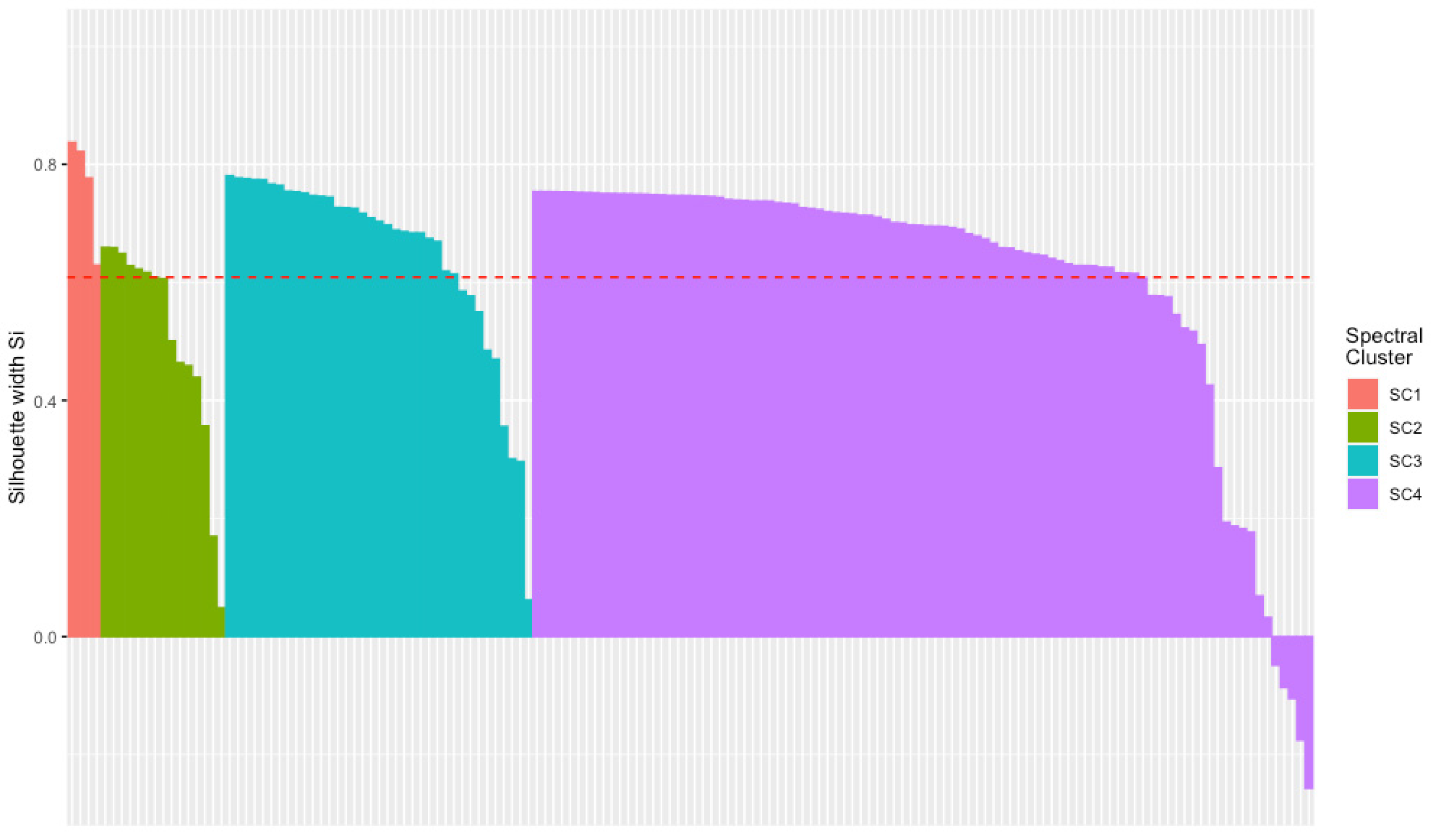
| Cluster | Number of Teams | Team ID | Silhouette Index |
|---|---|---|---|
| SC1 | 4 | 53, 12, 65, 10 | 0.77 |
| SC2 | 15 | 30, 2, 55, 50, 15, 54, 42, 86, 47, 21, 4, 73, 59, 69, 43 | 0.50 |
| SC3 | 37 | 133, 147, 135, 120, 150, 105, 67, 148, 68, 49, 84, 76, 20, 75, 81, 78, 40, 98, 14, 72, 85, 70, 61, 28, 16, 46, 74, 11, 89, 6, 94, 144, 79, 44, 56, 124, 8 | 0.65 |
| SC4 | 94 | 131, 102, 63, 1, 101, 24, 48, 134, 110, 122, 140, 117, 129, 32, 90, 108, 112, 116, 18, 19, 38, 142, 145, 109, 37, 130, 83, 121, 128, 141, 41, 132, 103, 3, 93, 119, 62, 118, 138, 127, 87, 64, 106, 111, 115, 22, 35, 31, 91, 126, 96, 80, 143, 13, 92, 26, 29, 17, 9, 146, 149, 95, 100, 66, 52, 123, 51, 88, 45, 60, 39, 36, 33, 5, 25, 139, 113, 77, 27, 104, 137, 71, 99, 97, 82, 58, 23, 34, 136, 57, 114, 107, 125, 7 | 0.60 |
| Team_ID | Team | Tournament | Cluster | |
|---|---|---|---|---|
| 1 | 10 | Barcelona | La Liga | SC1 |
| 2 | 12 | Bayern Munich | Bundesliga | SC1 |
| 3 | 53 | Manchester City | Premier League | SC1 |
| 4 | 65 | Paris Saint Germain | Ligue 1 | SC1 |
| 5 | 2 | AC Milan | Serie A | SC2 |
| 6 | 4 | Arsenal | Premier League | SC2 |
| 7 | 15 | Borussia Dortmund | Bundesliga | SC2 |
| 8 | 21 | Chelsea | Premier League | SC2 |
| 9 | 30 | Fiorentina | Serie A | SC2 |
| 10 | 42 | Inter Milan | Serie A | SC2 |
| 11 | 43 | Juventus | Serie A | SC2 |
| 12 | 47 | Liverpool | Premier League | SC2 |
| 13 | 50 | Lyon | Ligue 1 | SC2 |
| 14 | 54 | Manchester United | Premier League | SC2 |
| 15 | 55 | Marseille | Ligue 1 | SC2 |
| 16 | 59 | Napoli | Serie A | SC2 |
| 17 | 69 | Real Madrid | La Liga | SC2 |
| 18 | 73 | Roma | Serie A | SC2 |
| 19 | 86 | Tottenham | Premier League | SC2 |
Disclaimer/Publisher’s Note: The statements, opinions and data contained in all publications are solely those of the individual author(s) and contributor(s) and not of MDPI and/or the editor(s). MDPI and/or the editor(s) disclaim responsibility for any injury to people or property resulting from any ideas, methods, instructions or products referred to in the content. |
© 2023 by the authors. Licensee MDPI, Basel, Switzerland. This article is an open access article distributed under the terms and conditions of the Creative Commons Attribution (CC BY) license (https://creativecommons.org/licenses/by/4.0/).
Share and Cite
Bond, A.J.; Beggs, C.B. Bisecting for Selecting: Using a Laplacian Eigenmaps Clustering Approach to Create the New European Football Super League. Mathematics 2023, 11, 720. https://doi.org/10.3390/math11030720
Bond AJ, Beggs CB. Bisecting for Selecting: Using a Laplacian Eigenmaps Clustering Approach to Create the New European Football Super League. Mathematics. 2023; 11(3):720. https://doi.org/10.3390/math11030720
Chicago/Turabian StyleBond, Alexander John, and Clive B. Beggs. 2023. "Bisecting for Selecting: Using a Laplacian Eigenmaps Clustering Approach to Create the New European Football Super League" Mathematics 11, no. 3: 720. https://doi.org/10.3390/math11030720
APA StyleBond, A. J., & Beggs, C. B. (2023). Bisecting for Selecting: Using a Laplacian Eigenmaps Clustering Approach to Create the New European Football Super League. Mathematics, 11(3), 720. https://doi.org/10.3390/math11030720