Article

Solar Energy Production Forecasting Based on a Hybrid CNN-LSTM-Transformer Model

1
Mathematics Department, College of Sciences, Tabuk University, Tabuk 71491, Saudi Arabia
2
Laboratory of Energetics and Thermal and Mass Transfer (LR01ES07), Faculty of Sciences of Tunis, University of Tunis El Manar, Tunis 1068, Tunisia
3
Remote Sensing Unit, College of Engineering, Northern Border University, Arar 91431, Saudi Arabia
4
Laboratory of Electronics and Microelectronics (LR99ES30), University of Monastir, Monastir 5019, Tunisia
5
Physics Department, College of Sciences, Tabuk University, Tabuk 71491, Saudi Arabia
6
College of Computer Sciences, King Khalid University, Abha 62529, Saudi Arabia
*
Author to whom correspondence should be addressed.
Mathematics 2023, 11(3), 676; https://doi.org/10.3390/math11030676
Submission received: 11 January 2023 / Revised: 23 January 2023 / Accepted: 27 January 2023 / Published: 28 January 2023
(This article belongs to the Special Issue Artificial Intelligence in Geoenvironmental and Energy Sciences)

Abstract

:
Green energy is very important for developing new cities with high energy consumption, in addition to helping environment preservation. Integrating solar energy into a grid is very challenging and requires precise forecasting of energy production. Recent advances in Artificial Intelligence have been very promising. Particularly, Deep Learning technologies have achieved great results in short-term time-series forecasting. Thus, it is very suitable to use these techniques for solar energy production forecasting. In this work, a combination of a Convolutional Neural Network (CNN), a Long Short-Term Memory (LSTM) network, and a Transformer was used for solar energy production forecasting. Besides, a clustering technique was applied for the correlation analysis of the input data. Relevant features in the historical data were selected using a self-organizing map. The hybrid CNN-LSTM-Transformer model was used for forecasting. The Fingrid open dataset was used for training and evaluating the proposed model. The experimental results demonstrated the efficiency of the proposed model in solar energy production forecasting. Compared to existing models and other combinations, such as LSTM-CNN, the proposed CNN-LSTM-Transformer model achieved the highest accuracy. The achieved results show that the proposed model can be used as a trusted forecasting technique that facilitates the integration of solar energy into grids.

1. Introduction

Modern cities require more energy than usual. As these cities are intended to be green, renewable energy resources are the alternative to provide the required energy. Integrating renewable energy into a grid provides enormous benefits to the economy and the environment by reducing greenhouse gas emission and energy production cost. However, renewable energy resources present many challenges, such as variability and seasonality, that directly affect their integration into a grid. Solar power is the most important renewable energy resource with high production and reliability. It presents low panel cost with high efficiency [1,2]. Considering the aforementioned advantages of solar energy, it is a growing renewable energy resource used worldwide in recent years [3].
For a safe and stable integration of solar energy into a grid, forecasting techniques have been deployed to estimate the generated energy and align it with the energy demanded. Precise forecasting can predict energy production values close to the real values [4]. Solar energy forecasting is very important for grid integration [5], reserve estimation, and storage management. Accurate forecasting requires high-performance techniques and historical data availability. Recent Deep Learning techniques have proven to be efficient for time-series forecasting and great results have been achieved. Besides, the availability of open datasets of historical time series for solar energy forecasting is very important.
Recent advances in Artificial Intelligence (AI) techniques have powered a wide range of applications, such as object detection [6], scene classification [7], transportation systems [8], and time-series forecasting [9]. Forecasting solar energy production is one of the most investigated applications based on AI techniques [10]. It has been proved that promising results can be achieved compared to other kinds of forecasting methods due to the ability of AI models to learn from historical data and build a strong relationship between relevant features. Traditional AI techniques, such as extreme learning machines [11], support vector machines [12], and fuzzy neural networks [13], are widely adopted to model the non-linear relationship relating time series with forecasting outputs. However, these models are characterized by a shallow structure with a limited learning capability. In addition, feature selection is based on handcrafted descriptors that require experienced engineering and prior domain knowledge. Thus, shallow models present many limitations for solar energy production forecasting, which requires high-performance models. Three main limitations prevent the use of shallow models for solving forecasting problems. First, handcrafted features require highly skilled engineers with prior knowledge of the domain of solar power production data. Since feature selection is based on unreliable engineering experience, shallow models are inappropriate for discovering non-linear features in variant historical time series of solar energy production. Second, shallow models have a low generalization capability. The performance of these models is proved for smooth applications with simple data. However, the historical time series of solar energy production is highly complex and variant due to noisy weather conditions. Thus, shallow models are not suitable for mapping complex relationships in solar energy production forecasting. Finally, shallow models achieve a high performance with small training datasets, but a lower performance is obtained with large-scale datasets due to the overfitting problem. Historical time series of solar energy production forecasting present large-scale datasets, which make shallow models unable to handle this amount of data. For example, the Autoregressive Integrated Moving Average (ARIMA) was applied for solar poser forecasting [14], and low performances were achieved. The aforementioned limitations drive the need for more powerful AI techniques, such as Deep Learning [15].
Deep Learning is a very powerful AI technique widely adopted for a wide range of applications. Deep Learning presents a high learning capacity from large-scale datasets, supports unsupervised learning, and has a high generalization capability. Compared to shallow models, it is more powerful and can handle more complex applications, such as indoor object detection [16], fatigue detection [17], and forecasting problems [18]. For solar energy production forecasting, many Deep Learning models, such CNN [19], LSTM [20], and autoencoders [21], have been successfully applied to solve the problem.
Recently, a new kind of model, named Transformers [22], was proposed for sequence-to-sequence modeling. It was originally designed for natural language processing applications and was then generalized to computer vision applications [23]. To the best of our knowledge, it has not been previously adopted for solar energy production forecasting. The main limitations that prevent the use of Transformers in time-series forecasting are the following:
  • Quadratic time computation: the main operation for the self-attention block proposed by Transformers, named canonical dot product [22], is computationally extensive and requires large memory storage.
  • Very large memory for large input: large input requires stacking more encoder/decoder layers, which results in the doubling of the required memory by a factor equal to the number of stacked encoder/decoder layers. This limits the use of Transformer for processing large inputs, such as long time series.
  • Low processing speed: the processing speed of the encoder/decoder structures works sequentially, which increases the processing time.
In this work, we focused on solving the aforementioned limitations to make Transformers more suitable for solar energy production forecasting. We improved a Transformer structure with new components, and we modified the self-attention block. Then, convolutional layers were integrated into the Transformer encoder structure. In addition, the LSTM network was adopted to enhance prediction performances. The proposed forecasting methods consist of a preprocessing stage based on the clustering technique. The self-organizing map algorithm [24] was used for clustering the input data based on seasons, which makes the data more useful. The hybrid CNN-LSTM-Transformer model was then used to forecast solar energy production. The experiments using the Fingrid open dataset [25] demonstrated the high performance of the proposed model compared to current state-of-the-art models and other combinations, such as LSTM-Transformer and CNN-Transformer.
The contributions of this study are as follows:
  • The proposed clustering technique increased the forecasting accuracy. The solar irradiation in the collected data presents wide variation between different seasons. Thus, clustering the data into four main clusters based on seasons enhanced the learning capacity of the proposed model.
  • The CNN-LSTM combination represented a more powerful forecasting model. CNN and LSTM are two powerful Deep Learning models for time-series forecasting. The combination of the two models was very effective for forecasting solar energy production.
  • Adopting a Transformer achieved a better performance. The proposed Transformer was very important for enhancing the performance of the CNN-LSTM combination. It was used to force the LSTM to pay attention to relevant features in the historical time series and to generate more accurate predictions.
  • Proposing a probe sparse operation was important to replace the canonical dot product operation in the self-attention block. The proposed operation reduced the computational time and storage memory.
  • Proposing a distillation technique helped privilege the dominating attention scores in the stacked encoder. This technique reduced the computational complexity and allowed the processing of longer sequences.
  • Proposing a generative decoder helped acquire long sequences through a simple forward pass. It was useful for preventing the spread of cumulative errors in the inference.
The rest of the paper is organized as follows: Section 2 presents related works. The proposed approach is described and detailed in Section 3. The experiments and results are presented and discussed in Section 4. In Section 5, the conclusions and directions for future works are provided.

2. Related Works

As the energy demand of modern cities grows fast, there is a need for a trusted forecasting system to smoothly integrate renewable energy into a grid. To this end, various methods have been proposed to build high-performance solar energy forecasting systems. In this study, only Deep Learning-based methods are discussed since they outperform old methods by a large margin.
A combination of an autoencoder and a bidirectional LSTM neural network was proposed for the day before the renewable energy forecasting [26]. The proposed model, named AB-Net, was used in a one-step forecast of renewable energy production for short-term horizons. To build a training dataset, data were collected from various renewable energy resources. Next, the collected data were denoised and cleaned. After preprocessing the data, the AB-net was applied for forecast generation. First, the autoencoder was applied to extract the discriminative features. Second, the bidirectional LSTM was used to generate a forest by learning the temporal features of the data. The evaluation of the AB-Net on public datasets has proved its efficiency.
Qu et al. [27] proposed a solar energy forecasting system based on a temporal distributed gated recurrent network. The proposed system was composed of three main parts. First, the daily fluctuation in the data was extracted using a linear model. Second, a scenario generation model was designed to generate linear forecasting trends. Finally, the proposed temporal distributed gated recurrent network was used to generate the final one-day-ahead forecasts of solar energy production. The training data were collected from a solar energy farm in southeastern China. The proposed method was evaluated using data collected from the same farm, and acceptable results were achieved.
The power of Convolutional Neural Networks and LSTM networks was combined by Agga et al. [28] to develop a powerful solar energy foresting algorithm. The CNN was used to extract spatial features from the historical time series. Then, the LSTM was used to extract temporal features and to provide the predictions of solar energy production. The hybrid CNN-LSTM was designed over different forward and backward time series. The data used for training and evaluating the proposed forecasting algorithm were collected from a photovoltaic plant in Morocco. The data include production records, weather data, and power consumption of generated power. The experimental results proved that the proposed CNN-LSTM algorithm can provide good forecast results.
Rai et al. [29] developed a forecasting system based on the fusion of a sequence-to-sequence autoencoder and a gated recurrent unit. The proposed system takes advantage of supervised and unsupervised learning. First, the sequence-to-sequence autoencoder extracts the mysterious relationships between non-linear data of historical time series. In addition, it decreases the reconstruction error and taps the important feature correlation. Second, the gated recurrent unit extracts the temporal features by exploiting the time dependency of the time series. The proposed system was evaluated for different forecasting durations, such as 24 h, 48 h, and 15 days. Compared to the most recent forecasting methods, the proposed system provides reliable performance.
To facilitate the integration of solar energy into a smart grid, a production forecasting system based on the combination of a convolutional graph and a variational autoencoder was proposed in [21]. The proposed system extracts the probability distribution functions forecasting future solar power production in a modeled weighted graph. It is proved that learning the probability distribution functions is very useful for generating accurate forecasts. For training and evaluating the proposed system, data were collected from a set of photovoltaic sites in California, US. Each site was modeled as a weighted graph, where each node was a power measurement and the edges represented the correlation. By extracting relevant features using graph spectral convolution, the proposed system predicts future solar power production. The experiments proved that the proposed system could provide good results.
Sabri et al. [30] proposed the use of a combination of gated recurrent units and CNN to forecast solar power. The proposed method relays on the extraction of temporal and special features to predict solar power production. First, the gated recurrent units are applied to extract the temporal features. Second, the CNN extracts the spatial features. Finally, an output layer combines the extracted features and generates the forecasting results. The data for the training and evaluation of the proposed method were collected from the Desert Knowledge Australia Solar Centre (DKASC). Four years of data from May 2017 to May 2021 were collected with a five-minute resolution. The data include generated power, current, temperature, humidity, diffuse horizontal radiation, global horizontal radiation, and other information. The experiments proved that the proposed method could provide acceptable forecasting accuracy.
A multi-region solar power prediction system was proposed in [31]. A combination of a LSTM model and a particle swarm optimization algorithm was proposed to predict solar power production. First, the particle swarm optimization algorithm was applied to extract relevant features for the training of the LSTM network. Second, the extracted features were combined with the data from the training dataset and were fed to the LSTM network. Different LASTM variants were tested to select the best model. It was proved that the bi-directional LSTM network has the best performance compared to other variants.
Considering the presented works, there is still space to improve the prediction accuracy to better optimize the integration of solar power in a grid. The research gap in solar power production forecasting can be summarized in three points. First, there are few works that take advantage of a Transformer model to make time-series forecasting. Second, the optimization of a Transformer model for use in solar power forecasting has not been studied. Finally, the combination of CNN, LSTM, and Transformer will be considered the key to find the main relation in a historical time series.

3. Proposed Approach

In this work, a solar energy production forecasting system was proposed based on the combination of a CNN model, an LSTM model, and a Transformer. First, the CNN part was charged with extracting spatial features. Second, the LSTM part was charged with extracting temporal features. Finally, the Transformer combines the extracted features and generated predictions based on an encoder–decoder structure. Before feeding data to the proposed model, a clustering technique was applied for data organization and management. The self-organizing map algorithm was used for clustering the input data based on seasons, which makes the data more useful. The overall workflow of the proposed system is presented in Figure 1.

3.1. Proposed Forecasting Model

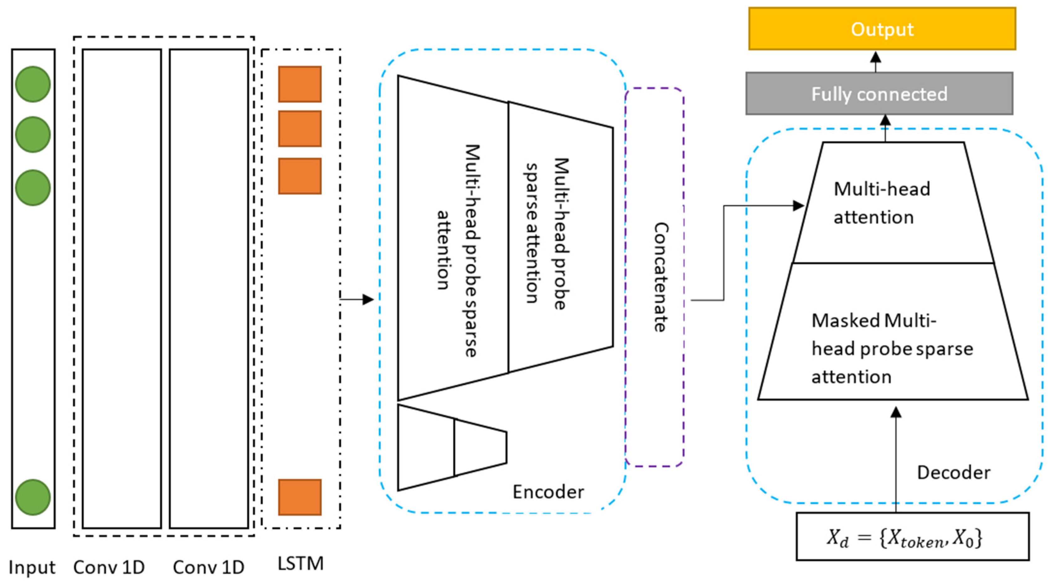
The proposed forecasting model consists of a CNN, a LSTM, and a Transformer. The CNN extracts the spatial features, the LSTM extracts the temporal features, and the Transformer employs the extracted features to generate the forecasting results. The transformer’s encoder–decoder strategy has the potential of improving forecasting accuracy by learning from the mixed spatial and temporal features.
The CNN model is composed of two convolution layers. The first layer has 16 convolution filters with a 3 × 1 kernel size. The second layer has 32 convolution filters with a 3 × 1 kernel. The LSTM model is composed of one layer with 32 units. The Transformer model is composed of three consecutive self-attention blocks with additional convolution, activation, and pooling layers. The proposed forecasting model is presented in Figure 2.

3.2. Self-Organizing Map Algorithm

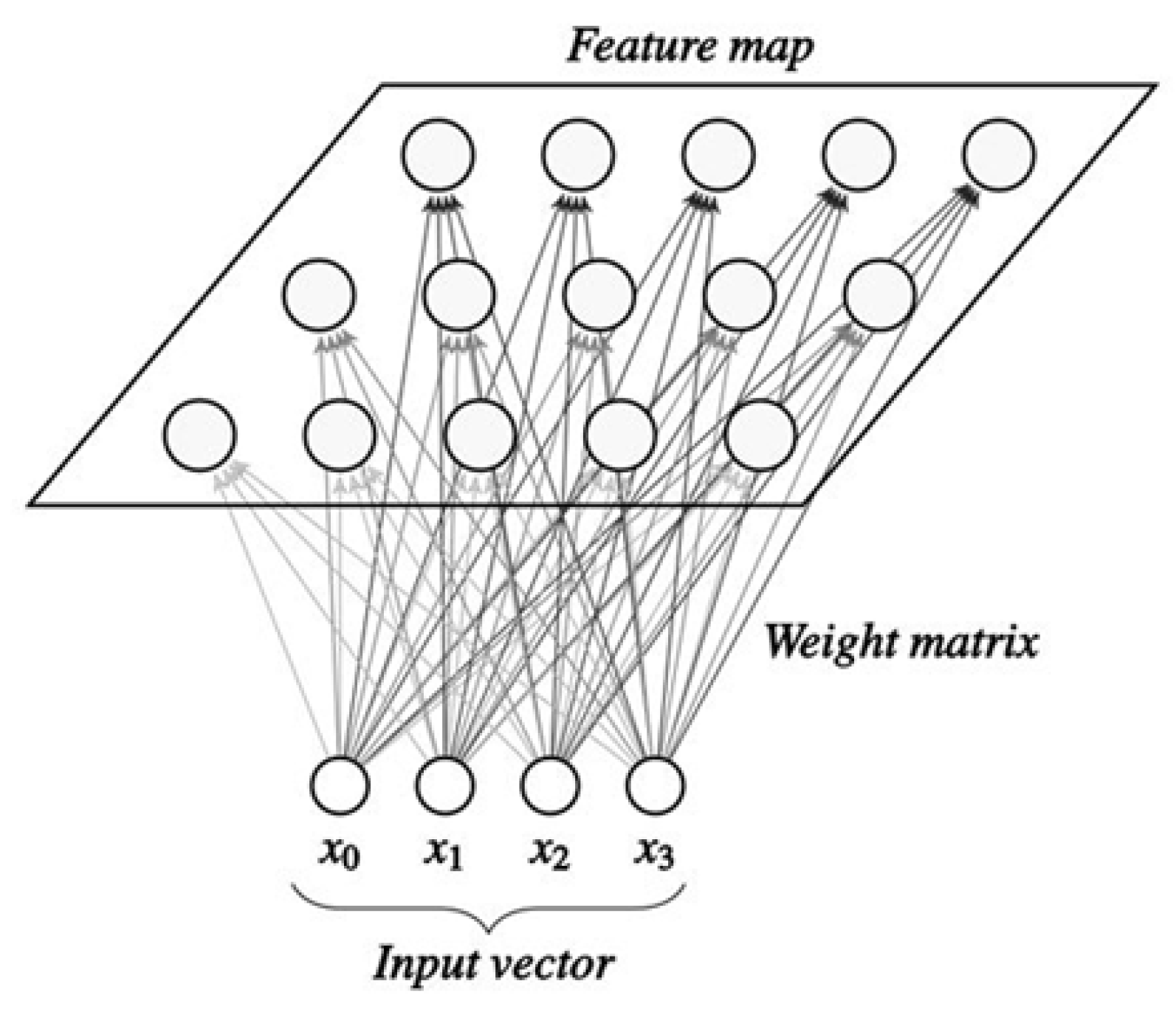
The main idea of clustering the input data is to regroup the data based on different seasons. Thus, the data were mapped into four clusters corresponding to four seasons. The data from the different clusters were used for training and evaluating the proposed system. For data clustering, a self-organizing map algorithm [32] was selected after testing many clustering algorithms. The main structure of the self-organizing map algorithm is presented in Figure 3.
The learning methodology of the self-organizing map algorithm is based on two main steps. First, the weight vector of each neuron in the feature map is normalized by the current vector x and the neuron value. Second, the winning neuron node is selected based on the minimum Euclidian distance between the neuron value and the weight. Then, the weight matrix is updated based on the new node. Updating the weight matrix can be computed using Equation (1) [32]:
w i j ( t + 1 ) = w i j ( t ) + η ( t ) h d , j ( t ) ( X i w i j ( t ) )
h d , j ( t ) = exp ( d d j 2 2 r 2 ( t ) )
r ( t + 1 ) = R N D ( ( r ( t ) 1 ) × ( 1 t T ) ) + 1
η ( t + 1 ) = η ( t ) η ( 0 ) T
where η ( t ) is the learning rate; w i j ( t + 1 ) is the updated weight; w i j ( t ) is the current weight; d d j 2 is the distance between neuron d and neuron j; r ( t ) is the neighborhood radius; T is the learning frequency; and RND is the rounding function.

3.3. Convolutional Neural Network

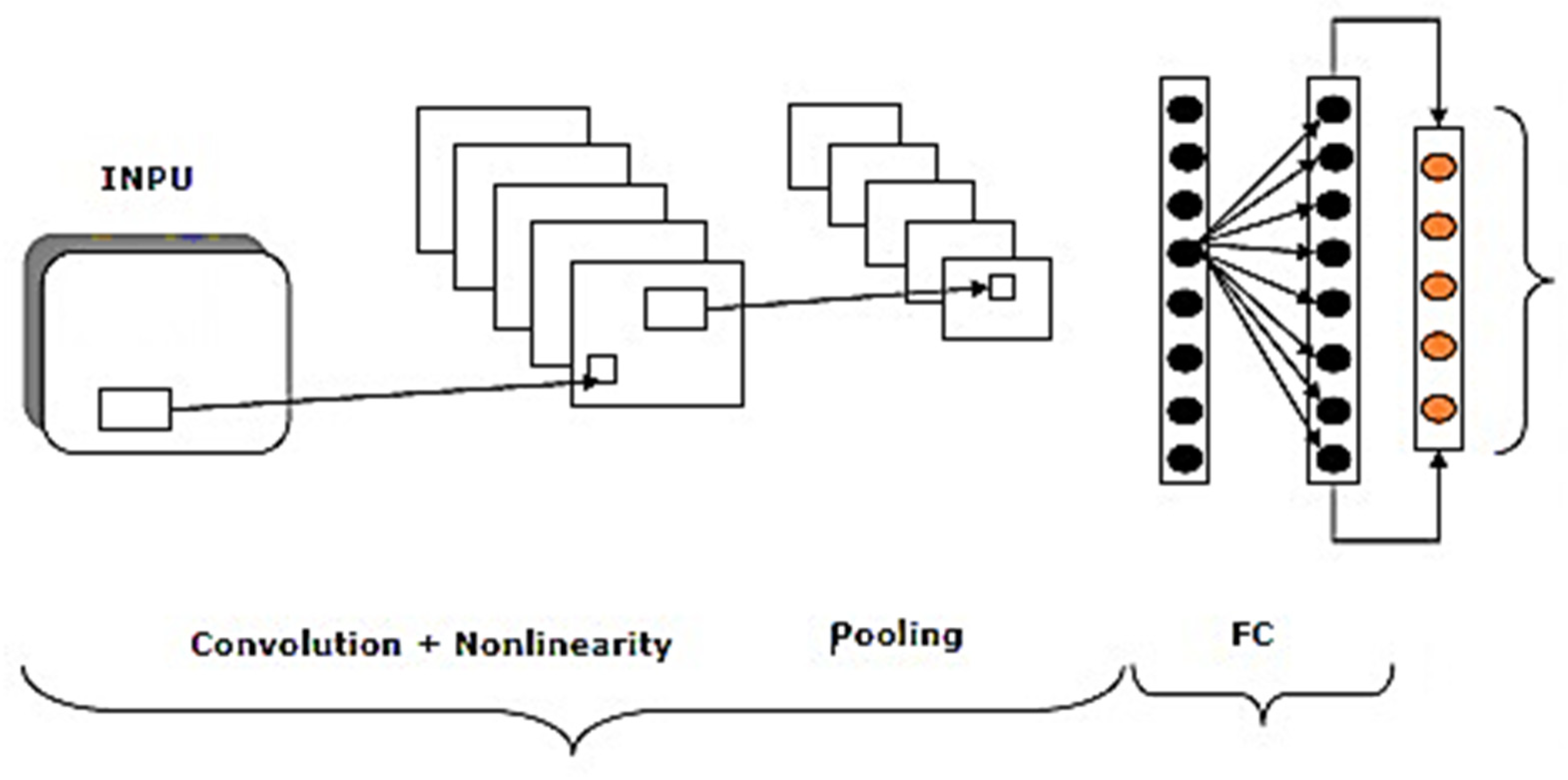
A Convolutional Neural Network (CNN) is one of the best Deep Learning models for solving different applications. A CNN model is based on four different layers, including convolution layers, activation layers, pooling layers, and fully connected layers. The convolution layers extract spatial features from the data; the activation layers enhance the learning capability by maximizing the non-linearity of the mapping function; the pooling layers compress the dimension of the feature maps; and the fully connected layers combine the global and local features extracted by the convolution layers. A typical representation of a CNN model is presented in Figure 4. For the problem of solar energy forecasting, a 1D convolution is used to process the time series. Considering a layer with input x i k and output y j k , the convolution layer is matrix multiplication between the input of the previous layer and a filter bank w i j k , while adding a regularization term (bias) b j k . The convolution layer can be computed using Equation (2):
y j k = i   ( x i k w i j k ) + b j k
In the nonlinear layer, a nonlinear activation function is applied, such as a rectified linear unit (ReLU). A nonlinear layer based on a ReLU can be computed as using Equation (3):
y ˜ j k = max ( 0 ,   y j k )
The maximum pooling layer is performed by selecting the maximum value in a given matrix. The fully connected layer can be dotted with a nonlinear activation function, such as a ReLU. The output layer for classification can be dotted with a softmax activation function, and for regression, it is dotted with a linear regression function. The softmax function can be computed using Equation (4), and the linear regression function can be computed using Equation (5):
p ( y j | x ) = e x T w j i = 1 k e x T w i
y = a x + b
where
a = n ( i = 0 n x i y i ) ( i = 0 n x i ) ( i = 0 n y i ) n ( i = 0 n x i 2 ) ( i = 0 n x i ) 2
b = ( i = 0 n y i ) a ( i = 0 n x i ) n

3.4. LSTM Unit

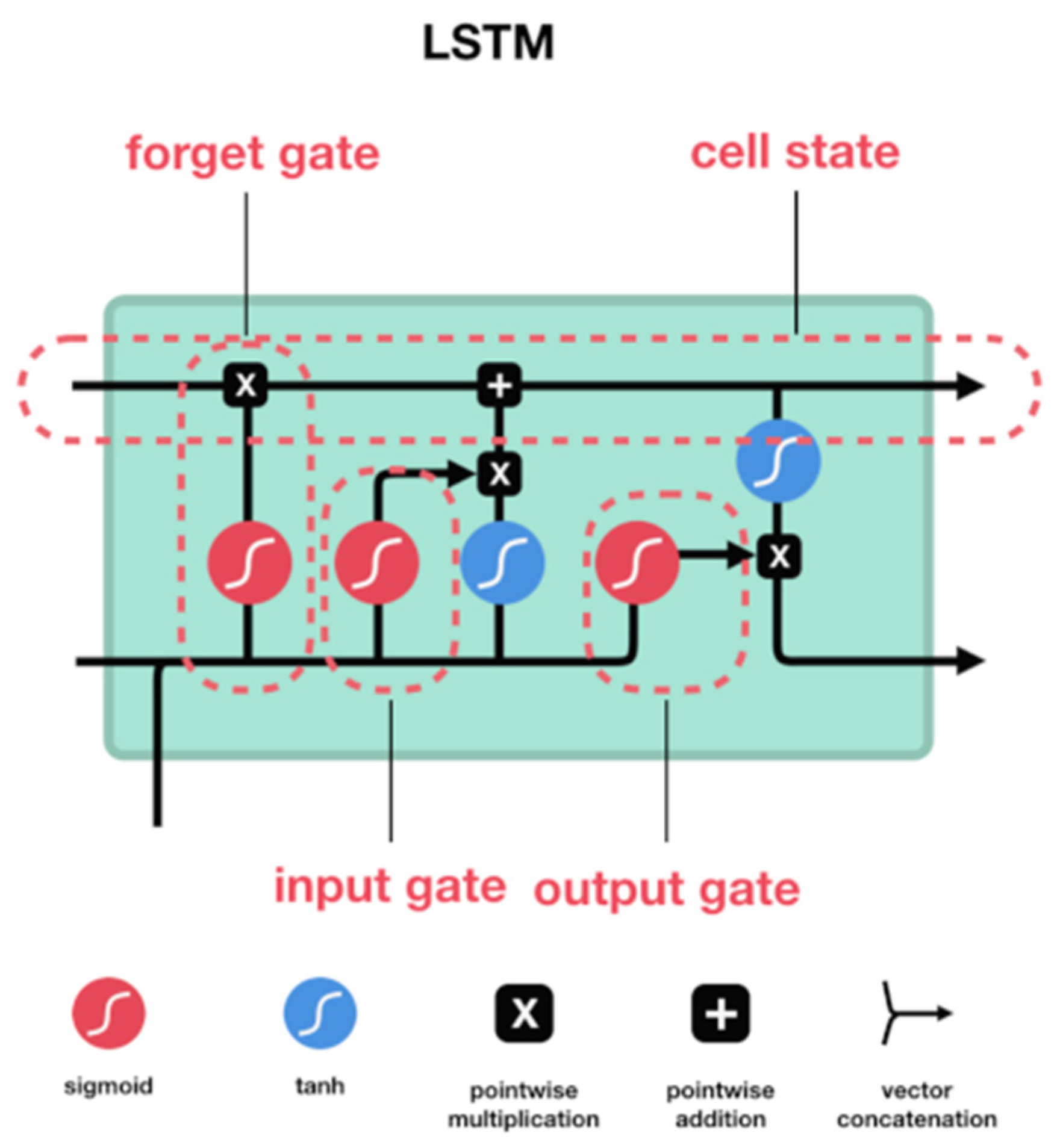
LSTM is a recurrent neural network variant, which was proposed to solve the vanishing gradient problem presented in older variants. An LSTM unit is based on three main gates, including the input gate, the forget gate, and the output gate, in addition to a cell state. A detailed illustration of an LSTM unit is presented in Figure 5. The input gate is charged with collecting information; the forget gate decides on the information to forget and store; and the output gate updates the unit value. These gates allow the control of information flow in the unit. This control presents an advantage for the problem of solar energy forecasting due to the possibility of continuously updating the unit based on a historical time series.
The LSTM unit can be computed by calculating the different gates. At instance t, the input gate is i t , the forget gate is f t , and the output gate is o t . The presented gates can be computed using (6):
i t = σ g ( w i x t + u i h t 1 + b i )  
f t = σ g ( w f x t + u f h t 1 + b f )
o t = σ g ( w o x t + u o h t 1 + b o )

3.5. Transformer

A Transformer presents a new kind of artificial neural network, which is mainly based on a self-attention mechanism. It was originally designed for natural language processing applications and was recently adopted for computer vision applications with the Vision Transformer (ViT) version. It mimics a recurrent neural network that processes sequential data but has different working processes. A Transformer processes all the data at once compared to a RNN that processes data sequentially. Transformers suffer from many problems that limit their use in solar energy forecasting. The main limitations can be summarized into the following three points:
  • Quadratic time computation: the main operation for the self-attention block proposed by Transformers, named canonical dot product, is computationally extensive and requires large memory storage.
  • Very large memory for large input: large input requires stacking more encoder/decoder layers, which results in the doubling of the required memory by a factor equal to the number of stacked encoder/decoder layers. This limits the use of Transformers for processing large inputs, such as long time series.
  • Low processing speed: the processing speed of the encoder/decoder structures works sequentially, which increases the processing time.
The canonical self-attention mechanism is based on three main inputs, which are the query (Q), the key (K), and the value (V). Considering an input with a dimension d, the output of the canonical self-attention mechanism can be computed using Equation (7):
A ( Q ,   K ,   V ) = s o f t m a x ( Q K T d ) V
The output for a specific raw in Q, K, and V can be computed using Equation (8):
A ( Q ,   K ,   V ) = j k ( q i ,   k j ) l k ( q i ,   k l ) v j = E p ( k j | q i ) [ v j ]
p ( k j | q i ) = k ( q i ,   k j ) l k ( q i ,   k l )
The self-attention mechanism processes the input values and generates the output by calculating the probability p ( k j | q i ) . This process requires quadratic time computation and memory storage in the order of O ( L K L Q ) . Enhancing the performance of the Transformer requires additional computation, which limits its use in real applications. Many works [33,34] have been proposed to overcome these limitations by discovering the sparsity of the probability distribution computed by the self-attention mechanism. Motivated by this discovery, a new kind of self-attention mechanism was proposed. To attend to this, we started by evaluating the learned attention patterns. It was discovered that only a few numbers of dot-product pairs affect the overall performance, while the others do not contribute to the performance. Thus, the main idea is to eliminate dot-product pairs that do not affect the performance.
Considering the query q i , the attention output on all keys is the composition between the probability p ( k j | q i ) and the V values. The corresponding query’s attention probability distribution is encouraged to deviate from the uniform distribution by the dominant dot-product pairs. If the probability p ( k j | q i ) is close to a uniform distribution equal to q ( k j | q i ) = 1 L K , then the output of the self-attention mechanism is the sum of the V values. To identify the relevant queries, the similarity between distributions p and q can be used. We proposed measuring the similarity using the Kullback–Leibler divergence method [35]. The similarity between q and p can be computed using Equation (9):
K L ( q | | p ) = l n l = 1 L K e q i k l T d 1 L K j = 1 L K q i k l T d l n L K
After eliminating the constant, the sparsity for the ith query can be computed using Equation (10):
M ( q i , K ) = l n l = 1 L K e q i k l T d 1 L K j = 1 L K q i k l T d
The query that obtains a high measure M ( q i , K ) has a high probability of containing the dominant dot-product pair that contributes to the overall performance. By considering this measurement, a probe sparse operation for self-attention was proposed to replace the canonical operation. The probe sparse operation allows the processing of a fixed number n of queries for each key. The attention based on the proposed operation can be computed using Equation (11):
A ( Q ,   K ,   V ) = s o f t m a x ( Q K T d ) V
Q contains n queries that satisfy the measurement M with the same size as q. A sampling factor c was proposed to control the number of queries n. Hence, the number of queries can be controlled based on Equation (12):
n = c × l n L Q
This relation reduces the calculation of dot-product operations for the query–key lookup to O ( l n L Q ) and maintains the memory occupation for each layer in the order of O ( L K l n L Q ) . The multi-head approach explains that this attention creates various sparse query–key pairings for each head, preventing significant information loss in return.
However, in order to process all of the queries for the measurement M, it is necessary to calculate each pair of dot products, and the first part of the measurement operation may have a problem with numerical stability. We suggest an empirical approximation for the effective acquisition of the query sparsity measurement to overcome this issue. As such, the measurement can be computed using Equation (13):
M ^ ( q i , K ) = max j   ( q i k l T d ) 1 L K j = 1 L K q i k l T d
The proposed max operator in measurement M ^ is less sensitive to zero values, in addition to presenting good numerical stability. Practically, the self-attention mechanism accepts equal input length for both queries and keys. Considering L as the input length, the computational complexity for the probe sparse based on self-attention is O ( L   l n   L ) .
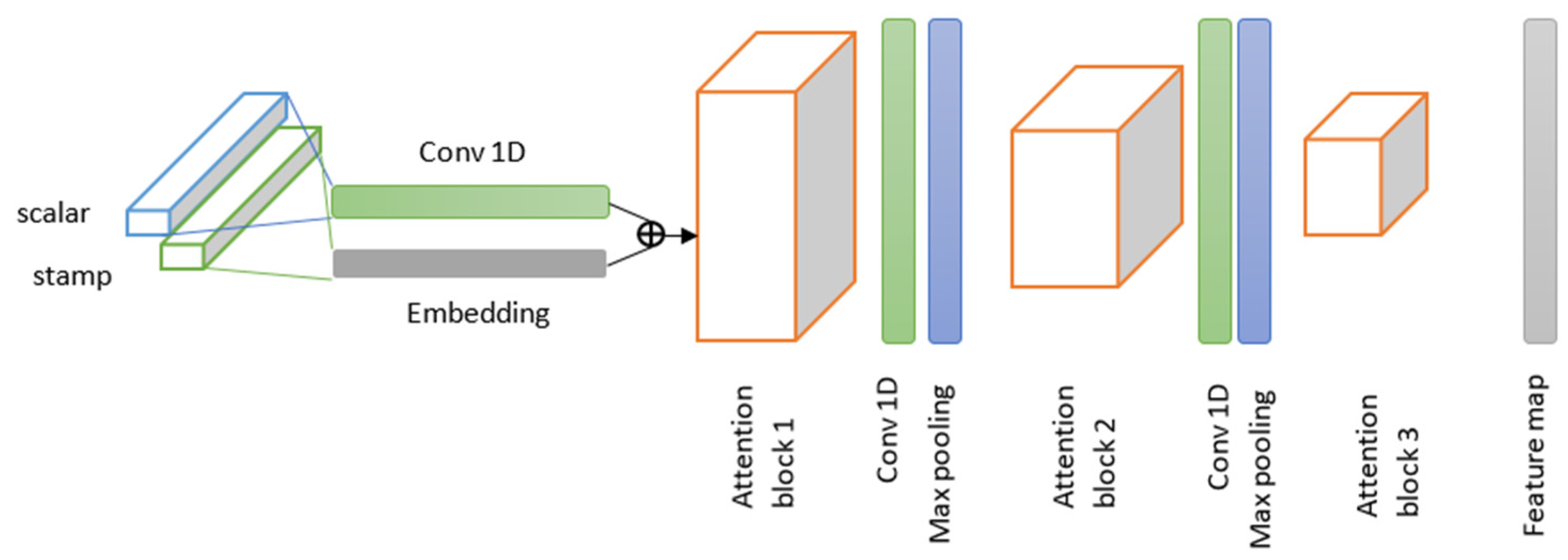
Memory limitation is a hard challenge that prevents the adoption of a Transformer in time-series forecasting. To overcome this limitation, we designed an encoder that processes longer sequential input, while requiring less memory. For this purpose, a new component was proposed based on the use of a 1D convolution layer and embedding the layer to generate the input of the self-attention block. The encoder’s purpose is to extract from the lengthy sequential inputs the reliable long-range dependency. The input is reshaped to matrix representation, the corresponding matrix for the tth input sequence X t is X m x t L x × d m .
Due to the use of the proposed probe sparse operation in the self-attention mechanism, the feature map of the encoder contains redundant combinations of value V. To handle this problem, a distilling operation was proposed to create a focused self-attention feature map in the next layer and to prioritize the better ones with dominant features. The proposed distilling operation was inspired by the dilated convolution [36]. Passing from one layer to the next one, the proposed distilling operation can be computed using Equation (14).
X j + 1 t = m a x p o o l ( E L U ( c o n v 1 D ( [ X j t ] A ) ) )
where maxpool represents the maximum pooling layer with a stride of 2; ELU is the exponential linear unit activation function; conv1D is a one-dimensional convolution layer with a kernel size of 3; and [ X j t ] A is the output of the proposed self-attention block. The proposed decoder structure is presented in Figure 6.
The proposed distilling operation reduces the memory occupation to O ( ( 2 ε ) L   l o g   L ) . In order to increase the robustness of the distilling process, we constructed copies of the main stack with the inputs reduced by half and gradually reduced the number of self-attention distilling layers by removing one layer at a time in a way that their output dimension is aligned. We then combined the outputs of each stack to obtain the encoder’s final hidden representation.
The next goal is to design a decoder that generates longer sequential outputs in a single forward way. We adopted the standard decoder of the Transformer model, which consists of two identical multi-head attention layers stacked on top of one another. The input vector of the decoder is computed using Equation (15):
X d t = c o n c a t   ( X t o k e n t ,   X 0 t ) ( L t o k e n + L y ) × d m
where X t o k e n t L t o k e n × d m is the start token and X 0 t L y × d m is the placeholder for the target sequence. In the Probsparse self-attention computing mechanism, the masked dot-products are set to , which implements masked multi-head attention. By preventing each position from anticipating the subsequent ones, auto-regressive behavior is avoided. To generate the output, a fully connected layer is used, with its size depending on the forecasting variate.
To achieve our goal, a generative inference was adopted by replacing specific flags as a token with L t o k e n input sequence and adding an earlier slice before the output sequence. In this way, the proposed decoder generates predictions in a single forward way instead of the dynamic decoding in the original transformer.
As a loss function, we proposed the use of the Mean Squared Error (MSE) function. The loss propagation starts from the decoder until reaching the input of the encoder.

4. Experiment and Results

The proposed model was extensively tested to prove its efficiency. The performance of the forecasting model was evaluated using a publicly available dataset. Different evaluation metrics were used for the evaluation of the model’s performance. In the next sections, we present the dataset used for training and evaluating the proposed forecasting model. In addition, we present the evaluation metrics used for evaluation. Besides, the achieved results are presented and discussed, and an ablation study is presented to prove the efficiency of the proposed model and the impact of the proposed components on the Transformer model.

4.1. Dataset

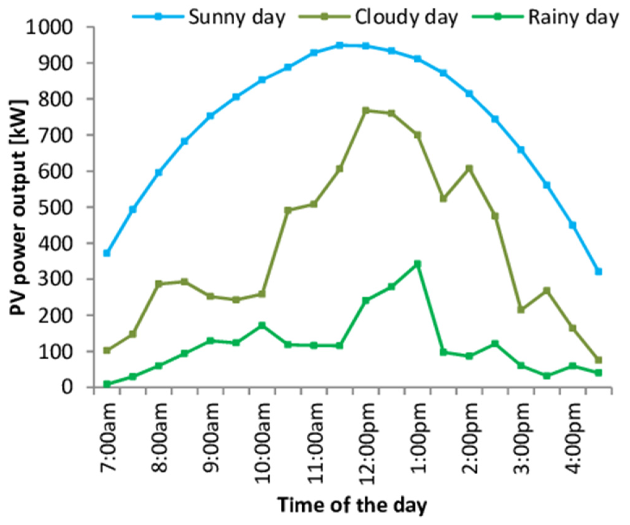
The Fingrid open dataset [25] was used to obtain the training data. The gathered data were updated at an hourly rate. The data were collected from a solar power plant established in Finland, which provided historical time series and weather conditions. The solar power plant can produce one megawatt of power per hour in total. The data were downloaded in the CSV format. Using the min-max normalization approach, the training data were normalized between zero and one. Data normalization enables performance comparisons without taking into consideration the solar power facility’s capacity. By excluding power levels throughout the night and on overcast days, the data were then filtered. After splitting the data into three sets, 60% were utilized for training, 10% were utilized for validation, and 30% were utilized for testing. A simple example of solar power prediction in relation to weather conditions, such as sunny, cloudy, and rainy, is presented in Figure 7.

4.2. Experimental Details

To find the most suitable hyperparameters for the proposed model, we applied a grid search technique. The proposed forecasting model is composed of a CNN with two 1D convolution layers, an LSTM layer, and a Transformer model. The CNN model has two convolution layers, where the first has 16 filters with a 3 × 1 kernel and the second one has 32 filters with the same kernel size. The LSTM is composed of 32 units. The Transformer model has an encoder with four stacked layers and a decoder with two layers. The proposed forecasting model was trained using the Adam optimizer with an initial learning rate of 0.0001. The learning rate was reduced to half every two epochs. The number of epochs was set to 10, with early stopping based on loss variation. The batch size was set to four due to the limited memory of the user environment, which is based on Nvidia GTX 960 GPU with 4 GB of memory. The input data were normalized to zero mean. A set of baseline forecasting models were selected for comparison, including the ARIMA [14], DeepAR [37], and prophet [38].

4.3. Evaluation Metrics

To evaluate the proposed CNN-LSTM-Transformer, three statistical evaluation metrics were used, including Root Mean Square Error (RMSE), Average Absolute Percentage Error (MAPE), and Mean Absolute Error (MAE). The used evaluation metrics can be computed using Equation (16).
MAE = ( i = 1 N | y ( i ) y ^ ( i ) | ) N
MAPE = ( i = 1 N | y ( i ) y ^ ( i ) / y ( i ) | ) N
RMSE = ( i = 1 N | y ( i ) y ^ ( i ) / y ( i ) | ² ) N 1
where y ( i ) is the target solar energy value and y ^ ( i ) is the predicted solar energy value. N is the number of samples.
The defined evaluation statistical tests were used to assess the forecasting system’s efficacy. The variation in assessment measures provides insight into the stability of the suggested model. The forecasting system deviates significantly from the target power output if the RMSE is very high when compared to the MAE. The forecasting system has a modest deviation from the goal power value if the RMSE is approximately equal to the MAE.

4.4. Results and Discussion

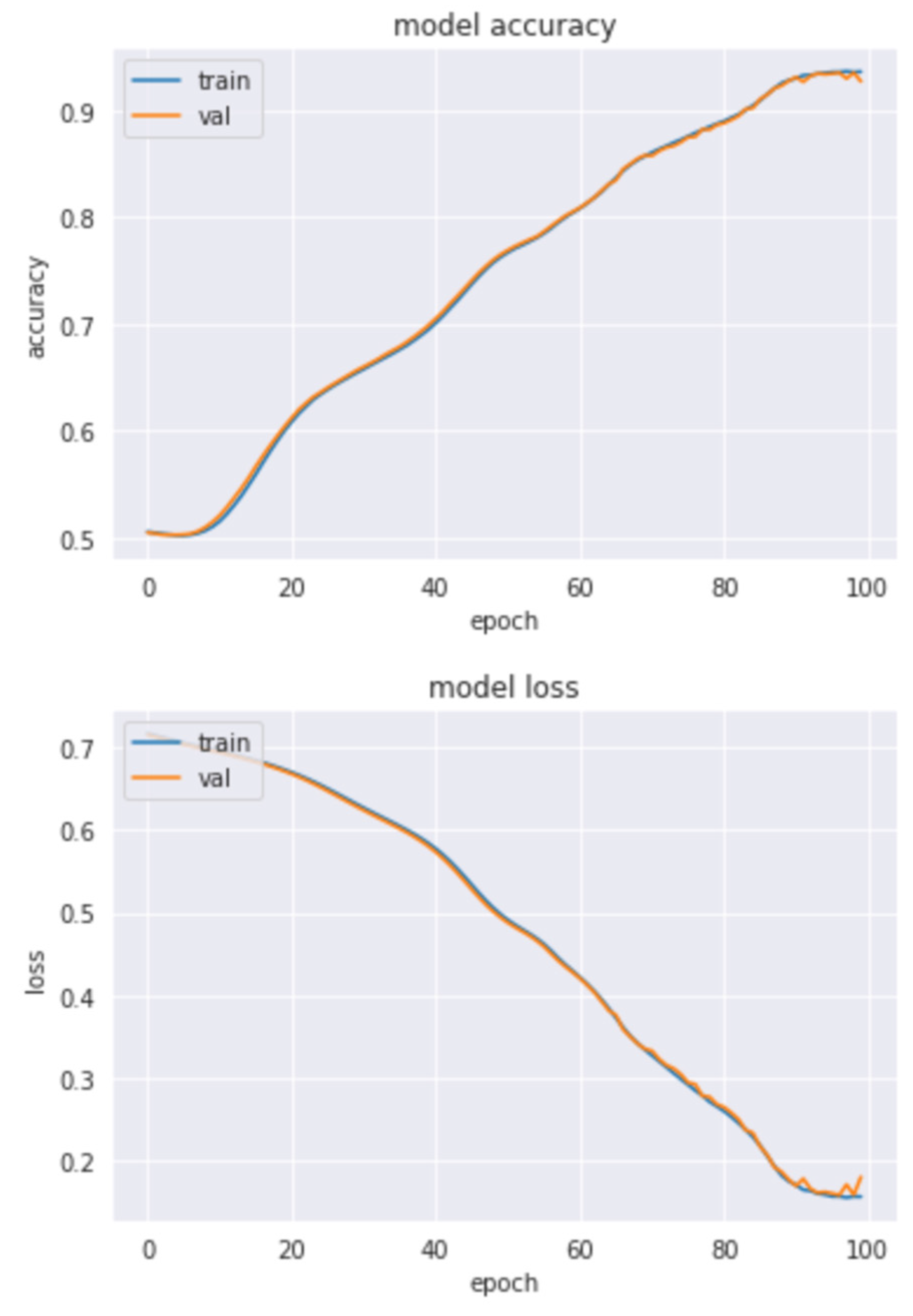
The proposed model was successfully trained and achieved a good loss minima and a high training accuracy. The curves of the model loss and training accuracy are presented in Figure 8.
The achieved results are presented in Table 1. To prove the efficiency of the proposed model, its performance with the original canonical self-attention was reported. The performance of the proposed model highlights the great impact of the probe-sparse self-attention module. The forecasting performance is further improved when compared to the original canonical self-attention. The proposed model achieves the lowest RMSE value, which reflects its high forecasting accuracy. The MAE presents the actual error situation on prediction value. The achieved results prove that the proposed model has a great capability in predicting solar power prediction.
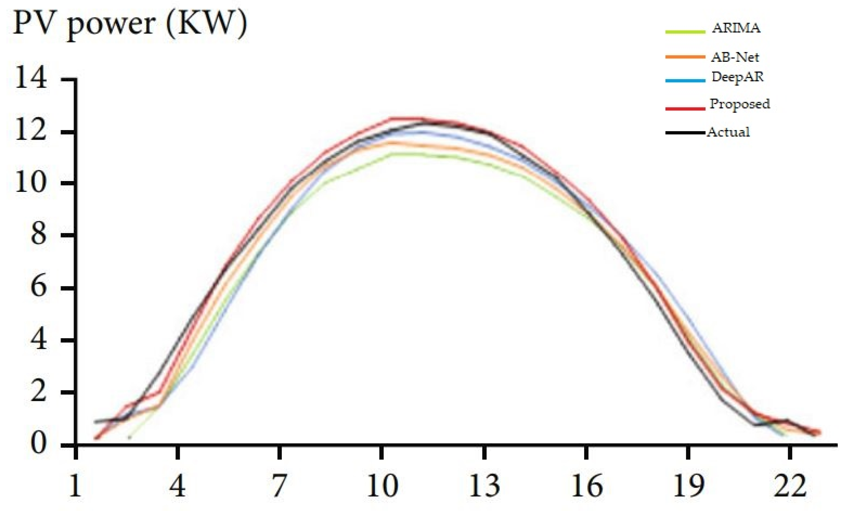
Referring to the results presented in Table 1, it can be noticed that the proposed CNN-LSTM-Transformer model achieves the top inference performance compared to the baseline models and compared to the variant based on canonical self-attention. This achievement proves the efficiency of the proposed assumption about query sparsity. It is very useful for generating more powerful attention feature maps. In addition, the proposed model outperforms current state-of-the-art forecasting models and provides more accurate predictions. These results prove the efficiency of combining a CNN, a LSTM, and a Transformer for solving the solar energy production forecasting problem. An example of solar power prediction for a time scale of one day comparing our model to current state-of-the-art models is presented in Figure 9. The proposed mode has the best prediction, which is closest to the actual value of solar power production.

4.5. Ablation Study

An ablation study was conducted to show the impact of each component in the proposed forecasting model. In this study, we focused on evaluating the impact of the proposed components in the Transformer model.
Impact of the probe-sparse self-attention mechanism: as shown in Table 1, the proposed probe-sparse self-attention mechanism outperforms the canonical self-attention mechanism. To avoid the memory efficiency problem, some model setups were reduced, such as the batch size was reduced to two, the number of heads was reduced to eight, and the dimension was reduced to 32, while other settings were fixed. Table 2 presents the achieved results with different input sizes and prediction lengths. It is obvious that our probe-sparse self-attention mechanism outperforms the canonical self-attention mechanism. The X in Table 2 refers to the memory failure of the model in our experimental environment. This ablation study proved the superiority of the proposed probe-sparse self-attention mechanism when being memory efficient.
Impact of the distilling operation: to prove the efficiency of the proposed distilling operation, we eliminated the probe-sparse self-attention mechanism and worked with the canonical self-attention mechanisms, while keeping other settings fixed. Table 3 presents the achieved results with and without the distilling operation. The model with the distilling operation has improved performance. The impact of the distilling operation is shown especially with longer prediction sequences. The model without the proposed distilling operation presents memory failure.
Impact of the proposed decoder: in the Transformer, the basic encoder–decoder structure is very important. We have already presented the impact of the different parts of the encoder. Here, we demonstrate the potential use of our decoder in obtaining generative outcomes. To this end, we eliminated the probe-sparse self-attention mechanism and the distilling operation to show the real impact of the generative decoder. Unlike previously proposed decoders, which require an alignment of the labels and the outputs during training and inference, the prediction of our suggested decoder is only based on the time stamp, which may forecast with offsets. The reported results in Table 4 prove that the proposed decoder can resist the increase in the offset, while the original decoder fails and presents memory failure with longer predictions. This demonstrates that the proposed decoder has a higher capacity in detecting long-range dependency by processing arbitrary outputs. Besides, it is very efficient in avoiding error accumulation.

4.6. Computational Efficiency

To show the efficiency of the proposed model in terms of computational complexity, a comparison study was performed between the proposed self-attention block and the original self-attention block of the transformer. Table 5 summarizes the achieved results for training and inference speed in addition to memory occupation. Based on the achieved results, the proposed model based on the probe-sparse self-attention mechanism is computationally efficient compared to the original canonical self-attention mechanism. The proposed model can be used for solar power forecasting to smoothly facilitate power integration in a grid. The proposed model is able to process large input time series, in addition to generating long output sequence, without requiring huge amounts of storage memory. The achieved inference speed allows the generation of reliable predictions in acceptable time for real-world applications.

5. Conclusions

Predicting photovoltaic power generation is critical for preserving system security and coordinating resource usage. Building a high-performance forecasting model is possible through recent advances in Artificial Intelligence techniques. Besides, the availability of large-scale datasets for historical time series is very important. In this paper, we proposed a forecasting model by combining a CNN, a LSTM, and a Transformer model. Unlike existing models, the proposed model presents effective techniques to reduce computational complexity while achieving higher performance. Besides, an effective preprocessing technique, such as the clustering technique, significantly enhances the performance of the proposed model. The CNN is employed to extract the spatial features, the LSTM is used to extract the temporal features, and the Transformer combines the extracted features and generates predictions based on the encoder–decoder structure. Many contributions were proposed to take advantage of the Transformer model for solar energy forecasting. The extensive experimentation proved the efficacy of the proposed model, which outperforms current state-of-the-art forecasting models. The proposed model achieved the lowest RMSE and MAE values of 0.344 and 0.393, respectively, compared to the Transformer-based models, Deep Learning-based model, and traditional models. The achieved results reflect the high accuracy of the model in forecasting solar power production. The main limitation is the complex training process. For future work, the proposed method can be extended for long-term forecasting, such as days or weeks. In addition, the use of the proposed model can be extended to forecast energy consumption and solar irradiations.

Author Contributions

Conceptualization, Y.H. and M.H.; methodology, M.A. and Y.S.; software, Y.S. and Y.H.; validation, M.H. and A.M.A.; formal analysis, A.H.L.; investigation, A.M.A.; resources, E.M.A.-A.; data curation, Y.S.; writing—original draft preparation, Y.S., Y.H. and E.M.A.-A.; writing—review and editing, M.A. and A.H.L.; visualization, Y.H.; supervision, Y.S.; project administration, E.M.A.-A. and Y.S.; funding acquisition, E.M.A.-A. All authors have read and agreed to the published version of the manuscript.

Funding

This research was funded by the Deanship of Scientific Research at the University of Tabuk through Research no. S-1443-0260.

Data Availability Statement

Data will be made available by the corresponding author upon request.

Acknowledgments

The authors extend their appreciation to the Deanship of Scientific Research at the University of Tabuk for funding this work through Research no. S-1443-0260.

Conflicts of Interest

The authors declare no conflict of interest.

Nomenclature

CNNConvolutional Neural Network
LSTMLong Short-Term Memory
AIArtificial Intelligence
DKASCDesert Knowledge Australia Solar Centre
RNDRounding function.
QQuery
KKey
VValue
ARIMAAutoregressive Integrated Moving Average
RMSERoot Mean Square Error
MAPEAverage Absolute Percentage Error
MAEMean Absolute Error

References

  1. Renewable Power Generation Costs in 2019. Available online: https://www.irena.org/publications/2020/Jun/Renewable-Power-Costs-in-2019 (accessed on 15 December 2022).
  2. Hajji, Y.; Bouteraa, M.; Elcafsi, A.; Bournot, P. Green hydrogen leaking accidentally from a motor vehicle in confined space: A study on the effectiveness of a ventilation system. Int. J. Energy Res. 2021, 45, 18935–18943. [Google Scholar] [CrossRef]
  3. IRENA (International Renewable Energy Agency). Future of Solar Photovoltaic: Deployment, Investment, Technology, Grid Integration and Socio-Economic Aspects; IRENA: Abu Dhabi, United Arab Emirates, 2019; pp. 1–73. [Google Scholar]
  4. Hajji, Y.; Bouteraa, M.; Bournot, P.; Bououdina, M. Assessment of an accidental hydrogen leak from a vehicle tank in a confined space. Int. J. Hydrogen Energy 2022, 47, 28710–28720. [Google Scholar] [CrossRef]
  5. Variable Renewable Energy Forecasting: Integration into Electricity Grids and Markets: A Best Practice Guide. Available online: https://cleanenergysolutions.org/resources/variable-renewable-energy-forecasting-integration-electricity-grids-markets-best-practice (accessed on 15 December 2022).
  6. Ayachi, R.; Said, Y.; Atri, M. A Convolutional Neural Network to Perform Object Detection and Identification in Visual Large-Scale Data. Big Data 2021, 9, 41–52. [Google Scholar] [CrossRef] [PubMed]
  7. Afif, M.; Ayachi, R.; Said, Y.; Atri, M. Deep Learning Based Application for Indoor Scene Recognition. Neural Process. Lett. 2020, 51, 2827–2837. [Google Scholar] [CrossRef]
  8. Ayachi, R.; Afif, M.; Said, Y.; Ben Abdelaali, A. Real-Time Implementation of Traffic Signs Detection and Identification Application on Graphics Processing Units. Int. J. Pattern Recognit. Artif. Intell. 2021, 35, 2150024. [Google Scholar] [CrossRef]
  9. Wang, K.; Qi, X.; Liu, H. Photovoltaic power forecasting based LSTM-Convolutional Network. Energy 2019, 189, 116225. [Google Scholar] [CrossRef]
  10. Wang, H.; Lei, Z.; Zhang, X.; Zhou, B.; Peng, J. A review of deep learning for renewable energy forecasting. Energy Convers. Manag. 2019, 198, 111799. [Google Scholar] [CrossRef]
  11. Alia, M.; Prasad, R. Significant wave height forecasting via an extreme learning machine model inte-grated with improved complete ensemble empirical mode decomposition. Renew. Sustain. Energy Rev. 2019, 104, 281–295. [Google Scholar] [CrossRef]
  12. Deo, R.C.; Wen, X.; Qi, F. A wavelet-coupled support vector machine model for forecasting global incident solar radiation using limited meteorological dataset. Appl. Energy 2016, 168, 568–593. [Google Scholar] [CrossRef]
  13. Sharifian, A.; Ghadi, M.J.; Ghavidel, S.; Li, L.; Zhang, J. A new method based on Type-2 fuzzy neural network for accurate wind power forecasting under uncertain data. Renew. Energy 2018, 120, 220–230. [Google Scholar] [CrossRef]
  14. Sharif, A.; Noureen, S.; Roy, V.; Subburaj, V.; Bayne, S.; Macfie, J. Forecasting of total daily solar energy generation using ARIMA: A case study. In Proceedings of the 9th Annual Computing and Communication Workshop and Conference (CCWC), Las Vegas, NV, USA, 7–9 January 2019; pp. 114–119. [Google Scholar]
  15. Feng, Q.; Chen, L.; Chen, C.L.P.; Guo, L. Deep learning. High-Dimensional Fuzzy Clustering. IEEE Trans. Fuzzy Syst. 2020, 28, 1420–1433. [Google Scholar]
  16. Afif, M.; Ayachi, R.; Said, Y.; Atri, M. An evaluation of EfficientDet for object detection used for indoor robots assistance navigation. J. Real Time Image Process. 2022, 19, 651–661. [Google Scholar] [CrossRef]
  17. Ayachi, R.; Afif, M.; Said, Y.; Ben Abdelali, A. Drivers Fatigue Detection Using EfficientDet In Advanced Driver Assistance Systems. In Proceedings of the 18th International Multi-Conference on Systems, Signals & Devices, Monastir, Tunisia, 22–25 March 2021; pp. 738–742. [Google Scholar] [CrossRef]
  18. Ayoobi, N.; Sharifrazi, D.; Alizadehsani, R.; Shoeibi, A.; Gorriz, J.M.; Moosaei, H.; Khosravi, A.; Nahavandi, S.; Chofreh, A.G.; Goni, F.A.; et al. Time series forecasting of new cases and new deaths rate for COVID-19 using deep learning methods. Results Phys. 2021, 27, 104495. [Google Scholar] [CrossRef] [PubMed]
  19. El Alani, O.; Abraim, M.; Ghennioui, H.; Ghennioui, A.; Ikenbi, I.; Dahr, F.-E. Short term solar irradiance forecasting using sky images based on a hybrid CNN–MLP model. Energy Rep. 2021, 7, 888–900. [Google Scholar] [CrossRef]
  20. Harrou, F.; Kadri, F.; Sun, Y. Forecasting of Photovoltaic Solar Power Production Using LSTM Approach. In Advanced Statistical Modeling, Forecasting, and Fault Detection in Renewable Energy Systems; Intechopen: London, UK, 2020. [Google Scholar] [CrossRef] [Green Version]
  21. Saffari, M.; Khodayar, M.; Jalali, S.M.J.; Shafie-Khah, M.; Catalao, J.P.S. Deep Convolutional Graph Rough Variational Auto-Encoder for Short-Term Photovoltaic Power Forecasting. In Proceedings of the 2021 International Conference on Smart Energy Systems and Technologies (SEST), Vaasa, Finland, 6–8 September 2021; pp. 1–6. [Google Scholar] [CrossRef]
  22. Vaswani, A.; Shazeer, N.; Parmar, N.; Uszkoreit, J.; Jones, L.; Gomez, A.N.; Kaiser, Ł.; Polosukhin, I. Attention is all you need. Adv. Neural Inf. Processing Syst. 2017, 30, 1–11. [Google Scholar]
  23. Dosovitskiy, A.; Beyer, L.; Kolesnikov, A.; Weissenborn, D.; Zhai, X.; Unterthiner, T.; Dehghani, M.; Minderer, M.; Heigold, G.; Gelly, S.; et al. An image is worth 16x16 words: Transformers for image recognition at scale. arXiv 2020, preprint. arXiv:2010.11929. [Google Scholar]
  24. Kohonen, T. The self-organizing map. Comput. Intell. Res. Front. 1990, 78, 1464–1480. [Google Scholar] [CrossRef]
  25. Fingrid Solar Power Generation Search and Download Data. Available online: https://data.fingrid.fi/en/dataset/solar-power-generation-forecast-updated-every-hour/resource/8b6b8bff-0181-48e1-aa86-1af97f81ce5a (accessed on 15 September 2022).
  26. Khan, N.; Ullah, F.U.M.; Haq, I.U.; Khan, S.U.; Lee, M.Y.; Baik, S.W. AB-Net: A Novel Deep Learning Assisted Framework for Renewable Energy Generation Forecasting. Mathematics 2021, 9, 2456. [Google Scholar] [CrossRef]
  27. Qu, Y.; Xu, J.; Sun, Y.; Liu, D. A temporal distributed hybrid deep learning model for day-ahead distributed PV power forecasting. Appl. Energy 2021, 304, 117704. [Google Scholar] [CrossRef]
  28. Agga, A.; Abbou, A.; Labbadi, M.; El Houm, Y.; Ali, I.H.O. CNN-LSTM: An efficient hybrid deep learning architecture for predicting short-term photovoltaic power production. Electr. Power Syst. Res. 2022, 208, 107908. [Google Scholar] [CrossRef]
  29. Rai, A.; Shrivastava, A.; Jana, K.C. A robust auto encoder-gated recurrent unit (AE-GRU) based deep learning approach for short term solar power forecasting. Optik 2022, 252, 168515. [Google Scholar] [CrossRef]
  30. Sabri, M.; El Hassouni, M. A Novel Deep Learning Approach for Short Term Photovoltaic Power Forecasting Based on GRU-CNN Model. E3S Web Conf. 2022, 336, 00064. [Google Scholar] [CrossRef]
  31. Zheng, J.; Zhang, H.; Dai, Y.; Wang, B.; Zheng, T.; Liao, Q.; Liang, Y.; Zhang, F.; Song, X. Time series prediction for output of multi-region solar power plants. Appl. Energy 2020, 257, 114001. [Google Scholar] [CrossRef]
  32. Kohonen, T. Essentials of the self-organizing map. Neural Netw. 2013, 37, 52–65. [Google Scholar] [CrossRef] [PubMed]
  33. Child, R.; Gray, S.; Radford, A.; Sutskever, I. Generating long sequences with sparse transformers. arXiv 2019, preprint. arXiv:1904.10509. [Google Scholar]
  34. Shiyang, L.; Jin, X.; Xuan, Y.; Zhou, X.; Chen, W.; Wang, Y.X.; Yan, X. Enhancing the locality and breaking the memory bottleneck of transformer on time series forecasting. Adv. Neural Inf. Processing Syst. 2019, 32, 1–11. [Google Scholar]
  35. Joyce, J.M. Kullback-leibler divergence. In International Encyclopedia of Statistical Science; Springer: Berlin/Heidelberg, Germany, 2011; pp. 720–722. [Google Scholar]
  36. Yu, F.; Koltun, V. Multi-scale context aggregation by dilated convolutions. arXiv 2015, preprint. arXiv:1511.07122. [Google Scholar]
  37. David, S.; Flunkert, V.; Gasthaus, J.; Januschowski, T. DeepAR: Probabilistic forecasting with auto-regressive recurrent networks. Int. J. Forecast. 2020, 36, 1181–1191. [Google Scholar]
  38. Sean, J.T.; Letham, B. Forecasting at scale. Am. Stat. 2018, 72, 37–45. [Google Scholar]
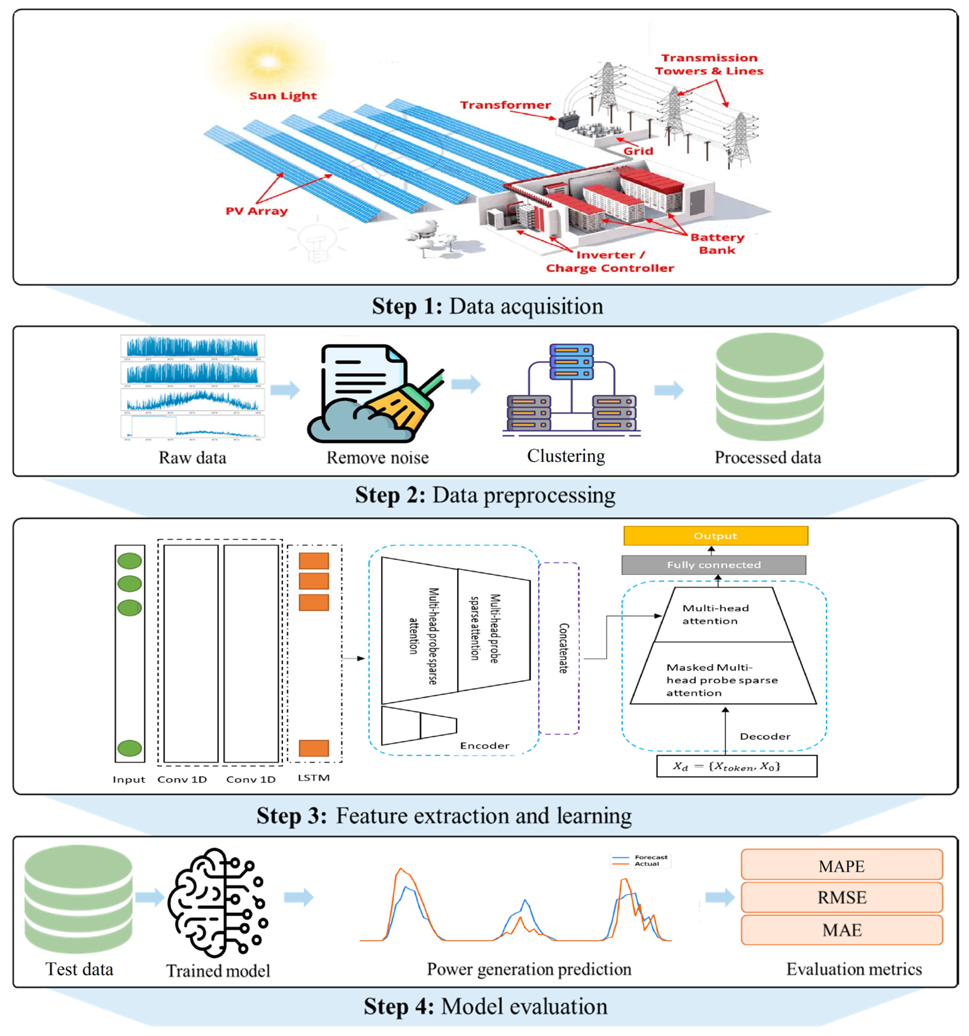
Figure 1. Overall workflow of the proposed system for solar power forecasting.
Mathematics 11 00676 g001
Figure 2. Proposed forecasting model.
Mathematics 11 00676 g002
Figure 3. Self-organizing map algorithm.
Mathematics 11 00676 g003
Figure 4. CNN model representation.
Mathematics 11 00676 g004
Figure 5. LSTM unit.
Mathematics 11 00676 g005
Figure 6. Proposed encoder structure.
Mathematics 11 00676 g006
Figure 7. Solar power prediction in relation to weather conditions.
Mathematics 11 00676 g007
Figure 8. Curves of the training and validation accuracies and losses.
Mathematics 11 00676 g008
Figure 9. Example of solar power forecasting on an hourly scale.
Mathematics 11 00676 g009
Table 1. Achieved results compared to baseline forecasting models.
ModelMAPEMAERMSE
CNN-LSTM-Transformer0.0410.3930.344
CNN-LSTM-Transformer *0.0480.3990.378
AB-Net [26]0.0520.4360.486
GRU-CNN [28]0.0530.4430.461
ARIMA [14]0.0730.7640.879
DeepAR [37]0.0510.4650.478
Prophet [38]0.0650.5240.598
CNN-LSTM-Transformer *: proposed model based on the canonical self-attention, CNN-LSTM-Transformer: proposed model based on probe-sparse self-attention.
Table 2. Ablation study of the probe-sparse self-attention mechanism.
Prediction Length336720
Input Size336720144072014402880
CNN-LSTM-TransformerRMSE0.2490.2250.2160.2710.2610.257
MAE0.3930.3840.3760.4350.4310.422
CNN-LSTM-Transformer *RMSE0.2510.234X0.285XX
MAE0.3990.398X0.442XX
CNN-LSTM-Transformer *: proposed model based on the canonical self-attention mechanism, CNN-LSTM-Transformer: proposed model based on probe-sparse self-attention mechanism.
Table 3. Ablation study on the distilling operation.
Prediction Length336480
Encoder Input336480720336480960
CNN-LSTM-Transformer * (with distilling)RMSE0.2490.2080.2250.1970.2430.192
MAE0.3930.3850.3840.3880.3920.377
CNN-LSTM-Transformer * (without distilling)RMSE0.2290.215X0.224XX
MAE0.3910.377X0.381XX
CNN-LSTM-Transformer *: proposed model based on the canonical self-attention mechanism.
Table 4. Ablation study on the generative decoder.
Prediction Length336480
Prediction Offset+0+12+24+0+48+96
CNN-LSTM-Transformer * (with generative decoder)RMSE0.2070.2090.2110.1980.2030.208
MAE0.3850.3870.3930.3900.3920.401
CNN-LSTM-Transformer * (without generative decoder)RMSE0.209XX0.392XX
MAE0.393XX0.484XX
CNN-LSTM-Transformer *: proposed model based on the canonical self-attention mechanism.
Table 5. Computational efficiency of the proposed model compared to the original canonical self-attention mechanism.
Prediction Length336
Input Size4896168
CNN-LSTM-TransformerTrain speed (hours)3.25.16.3
Inference speed (hours)0.10.130.17
Memory (GB)2.12.32.5
CNN-LSTM-Transformer *Train speed (hours)7.48.19.3
Inference speed (hours)0.30.380.42
Memory3.53.73.8
CNN-LSTM-Transformer: proposed model based on probe-sparse self-attention mechanism; CNN-LSTM-Transformer *: proposed model based on the canonical self-attention mechanism.
Disclaimer/Publisher’s Note: The statements, opinions and data contained in all publications are solely those of the individual author(s) and contributor(s) and not of MDPI and/or the editor(s). MDPI and/or the editor(s) disclaim responsibility for any injury to people or property resulting from any ideas, methods, instructions or products referred to in the content.