Lagrangian Heuristic for Multi-Depot Technician Planning of Product Distribution and Installation with a Lunch Break

Abstract

In this paper, we consider a technician planning scheme stemming from product distribution and installation in a manufacturing enterprise that considers factors such as soft time windows, skill areas, lunch breaks, and outsourcing options, among others. The goal is to identify the optimal partition of technicians into groups and assignment of customers to technician groups and find the optimal routes for technician groups to minimize the sum of the travel cost, soft time window violation cost, and outsourcing cost. To address this problem, the study develops a tailored Lagrangian heuristic that incorporates several strategies to speed up convergence and produce sharper bounds. Computational comparisons between the developed heuristic and MIP solver are presented. The results reveal that the bounds found by the developed algorithm outperform those found by CPLEX for large instances, and it is capable of identifying high-quality feasible solutions to large-scale problems.

1. Introduction

This study addresses a multi-depot technician planning problem stemming from product distribution and installation in a manufacturing enterprise, considering lunch breaks and soft time window constraints. The proposed solution aims to identify the optimal schedules for a certain number of service technicians to provide services at customers’ locations based on customer requests.

Specifically, we plan a horizon (a day), a set of service technicians located at different depots, and a set of customers associated with daily requests. Every technician qualifies in some areas at a different skill level (e.g., beginner, medium, or expert). Each service request requires a group of technicians with the appropriate skills with at least the required levels, and is associated with a time period during the day within which the request can be performed, which we refer to as a soft time window (STW). A violation of the time window is allowed, although it incurs some cost. Specifically, the STW violation cost is proportional to the delay incurred if the request is served after the soft time window is closed. However, the maximum delay of the customer is bounded.

On a given day, technicians from the same depot are paired with groups, the qualifications of which depend on the overall qualifications of group members. The groups then depart from the depot to serve customers by considering the compatibility between the group qualifications and requests, and return to it at the end of the day. Because technicians generally work approximately 6–8 h a day, every technician needs to break to rest and eat lunch, associated with which is a time window and a duration for the lunch break (Goel and Irnich [1]).

In addition, owing to the limited number of technicians and the limited working hours of each technician, in some cases, the service capacity of the supplier may not be sufficient to serve all customers. However, the service of unvisited customers still has to be provided, which may call for outsourcing the services to a third party or postponing them to the next planning period at an additional outsourcing cost.

The objective is to minimize the sum of the travel, STW violation, and outsourcing costs by identifying the optimal technician service schedule. The contributions of this study can be summarized as follows.

First, the present study introduces and describes a novel technician planning problem with several crucial features, including multiple depots, soft time windows, lunch-break requirements, and outsourcing options. These features make the developed problem closer to reality, but inevitably make the problem more difficult to solve. In fact, efficiently solving the problem with all of its features can be challenging, and an efficient algorithm that can find the optimal solution or approximate the optimal solution to the problem has not yet been developed. Therefore, this study aims to address this gap.

Second, we present a tailored Lagrangian heuristic to solve the developed model, incorporating several strategies to accelerate convergence and produce sharper bounds. More precisely, the revised volume algorithm is introduced to solve the Lagrangian dual problem, in which a bidirectional labeling algorithm is devised to optimally solve the Lagrangian subproblem. A two-stage hybrid heuristic is designed to transform the approximated primal solutions generated during the iterations of the Lagrangian heuristic into high-quality feasible solutions to the original problem.

Third, this study conducts several numerical experiments to verify the effectiveness and efficiency of the developed Lagrangian heuristic. The results demonstrate that the developed algorithm performs better than the general-purpose MIP solver CPLEX and can find relatively sharper bounds.

The remainder of this paper is organized as follows. Section 2 provides a brief review of the relevant literature. Section 3 defines the problem and draws up a mixed-integer programming formulation. Section 4 presents a Lagrangian heuristic with emphasis on the generation of the solution of the Lagrangian sub-problem and the strategies for transforming the approximated primal solutions into feasible solutions. Section 5 shows the computational results of applying the developed algorithm on newly generated instances based on the known benchmark instances in the literature. Finally, Section 6 concludes the paper by summarizing its findings and discussing future research directions.

2. Literature Review

Smart operation and maintenance services are major industrial services in Industry 4.0, but it is not easy for manufacturers to achieve high returns from these services due to their complex operational processes (Huang et al. [2]). Over the past decade, increasingly more practical features and constraints motivated by real-world settings have been addressed in technician planning problems. For example, as He et al. [3] pointed out, making an optimal equipment maintenance service plan is essential in enabling manufacturers to make more profit and avoid losing efficiency in the supply chain. Meanwhile, the service provider should cater to the needs of their customers and fully utilize their service skills to ensure a beneficial business (Orsdemir et al. [4]) The design of efficient technician routing and scheduling is challenging in this research area. In the following, we review the literature on technician planning problems in two main aspects: models and solution approaches. For more results on technician planning problems or related problems, the reader is referred to the survey papers by Castillo-Salazar et al. [5], Cissé et al. [6], and Fikar and Hirsch [7].

From a modeling point of view, the major differences among different models lie in the considered features, such as the working time regulations for technicians, customer preferences (time windows, skill and qualification requirements for the technicians), technician breaks, balancing the number of customers served by technicians, etc. The first study on technician planning can be traced to Dutot et al. [8], who investigated a real telecommunication problem. The authors focused on partitioning technicians into groups and assigning tasks to groups so that the skill and qualification requirements could be matched. This issue has subsequently been widely studied in various fields, such as production workshops, supply chains, healthcare, and so on, obtaining a myriad of valuable managerial insights. For example, Chen et al. [9] zeroed in the problem of assigning technicians to maintenance tasks at an aircraft maintenance base, in which the technician’s licenses, fairness, and operational constraints, such as hangar capacity and work shifts, are considered. They formulated the problem as a bi-objective optimization model with the aim of minimizing the total cost while simultaneously achieving fairness in workload allocation among different technicians. However, no routing decision is considered in these situations. Based on the study by Dutot et al. [8], the French Operations Research Society provided a real-world data set for technician planning problems in 2007. To solve the 2007 challenge, Cordeau et al. [10] developed a construction heuristic and an adaptive large neighborhood search to solve the technician planning problem with several features, including technician availability, customers’ skill requirements, precedence constraints, and working time regulations. The objective is to identify an optimal strategy for partitioning technicians into groups and assigning requests to groups to minimize the makespan. Kovacs et al. [11] studied the technician planning problem with an outsourcing option, which generalizes the problem investigated in Cordeau et al. [10] by including the routing decisions, where both cases with group building and without group building are considered. This problem differs from the present study in the settings of the depots and time windows in that no lunch break requirement is considered. Zamorano and Stolletz [12] investigated the multi-period technician planning problem to determine the daily partition of technicians into groups, the assignment of customers to groups, and the daily routes of the groups to minimize the sum of the travel cost, waiting cost, and over-time cost. In contrast to this problem, however, only a single depot and hard time windows are involved, and no lunch break requirement nor outsourcing option are considered. Chen et al. [13] studied the multi-period technician planning problem in the field of home services and consider the fact that the service time with the customer decreases as technicians’ experience increases, where the time needed for a technician to serve a request depends on the technician’s experience in the request-related skill and the speed at which the technician learns (the technicians’ learning rate). Qiu et al. [14] investigated a novel home healthcare (HHC) provider planning problem that considers the synchronized services of multiskilled providers necessitated by the simultaneous service requirements of patients. A main feature of the problem is that there is a threshold on the maximum difference between the start times of the pairwise synchronized services at a patient, which enables flexible imposition of various synchronization constraints and generalizes the setting of synchronized services in existing literature. They devised a tailored branch-and-price-and-cut solution algorithm that incorporates some enhancement strategies to solve the problem. Schrotenboer et al. [15] examined the technician planning problem for offshore wind farms over multiple periods to find the ships’ routes for picking up and delivering technicians at each period to minimize the travel cost. Both of the above problems, however, differ from this study’s problem in that customers can be visited at any time (no time windows), and no group-building decision or outsourcing option was considered. In addition, neither of these studies involved a lunch-break requirement. Liu et al. [16] studied the pickup and delivery problem with time windows involving battery-powered electric vehicles under demand uncertainly, where the uncertain demands fall within a budget polytope uncertainty set, and developed a two-stage adaptive robust model to find solutions that are insusceptible to a certain number of deviations in demands, where the routing, and the service start times and remaining battery capacities along a route are fixed before the realization of uncertain demands, while the quantities to load and unload along the route are adjustable to the demand scenario. Zou et al. [17] investigated the low-carbon multi-depot vehicle routing problem to minimize the sum of the vehicle assignment cost, travel cost, fuel consumption cost, and carbon emission cost, and developed a novel transformer model with both multi-head attention mechanism (MHA) and attention to attention mechanism (AOA) to solve the problem. In this model, the MHA is used to process different parts of the input sequence, which can be calculated in parallel, and the AOA is used to deal with the deficiency problem of correlation between query results and query vectors in the MHA.

Research on technician planning problems with lunch-break requirements is relatively scarce. Bostel et al. [18] investigated the multi-period technician planning problem to minimize the travel cost, in which several tasks are requested to be performed by a certain number of technicians over multiple days. Meanwhile, the features considered in this study included multiple depots, time windows, maximum daily working time, and lunch break requirements. Compared with our model, only some tasks are subject to the time window constraint, only technicians with identical skills at the same level are involved, and no outsourcing option nor group-building decision is studied. Shao et al. [19] addressed the therapist planning problem over multiple periods, in which the time windows and lunch-break requirements that occur when the consecutive working time of a therapist exceeds a given value are considered. The objective is to determine the optimal strategy of the assignment of patients to therapists over a week and the optimal daily routes of therapists to minimize the sum of the travel cost, mileage cost, treatment cost, and overtime cost. However, in their studies, only one depot is involved, all patients must be served, and no group-building decisions are involved. Trautsamwieser and Hirsch [20] investigated a HHC provider planning problem over a week, in which the working time regulations for HHC providers, including breaks, maximum daily working time, and daily and weekly rest times are involved. However, the break of a HHC provider at a patient’s home is only taken when their maximum consecutive working time is larger than a given value. Coelho et al. [21] addressed the vehicle routing problem with lunch break and time window constraints and assessed the performance of a new mathematical formulation and of the heuristic developed for the problem. Liu et al. [22] addressed a daily HHC giver planning problem with an outsourcing option, time windows, and lunch break requirements. The objective is to determine the optimal routes of HHC providers to minimize the sum of the travel and outsourcing costs. The two problems above, however, differ from our problem in that only a single depot and hard time windows are involved and no group-building decision is considered.

As for the solution approaches for the technician planning problems or related problems, branch-and-price algorithm (Bostel et al. [18], Cortés et al. [23], Goel and Irnich [1], Liu et al. [22], Trautsamwieser and Hirsch [20], Zamorano and Stolletz [12], Yuan et al. [24]) is commonly used to solve the problems of optimality in reasonable computing time. Since finding optimal solutions to the problems is only possible for small and medium-sized instances, they often become impossible or too slow when investigating more complex problem variants or real-sized instances. Heuristic methods are widely accepted, especially those that guarantee proximity to global optimality. Classical heuristics such as adaptive large neighborhood search (Cordeau et al. [10], Kovacs et al. [11], Schrotenboer et al. [15]), local search (Souffriau et al. [25]), TS (Tang et al. [26]), simulated annealing (Delgoshaei et al. [27]), and greedy randomized adaptive search (Hashimoto et al. [28], Shao et al. [19]) have been frequently applied to the technician planning problems or related problems. However, the primary drawback of these heuristics is the variability in solution quality across problem instances, and no lower bounds are provided to verify the quality of the solutions found. Instead, Lagrangian relaxation is a powerful bounding technique to provide sharper lower bounds and help derive high-quality feasible solutions for $NP$-hard combinatorial optimization problems, especially large-scale problems like Facility Location problems (Gendron et al. [29], Jena et al. [30]), Production problems (Cui et al. [31]), Inventory problems (Demantova et al. [32]), Logistics Network Design problems (Holmberg and Yuan [33], Lee and Dong [34]), Network Revenue Management problems (Topaloglu [35]), Stochastic Integer Programming problems (Takriti and Birge [36]), and others.

3. Problem Definition and Model Formulation

This section formally describes the problem under examination, and presents a mixed-integer linear programming model. The main notations are presented in

Table 1. Parameters and decision variables.

Sets
$\mathcal{H}$	Set of $\overline{h}$ depots, each of which corresponds to a customer’s location.
$\mathcal{N}$	Set of n service requests (customers), each of which corresponds to the location of a customer.
${\mathcal{A}}_h=\left\{(i,j)\right|i\in \mathcal{N}\cup \left\{h_o\right\},j\in \mathcal{N}\cup \left\{h_d\right\},i\ne j\}$	Set of arcs with $h_o$ and $h_d$ being the dummy vertexes of depot $h\in \mathcal{H}$.
${\mathcal{M}}_h$	Set of technicians living close to depot $h\in \mathcal{H}$.
$\mathcal{D}$	Set of different areas of skill of each technician.
$\mathcal{L}$	Set of different levels of proficiency associated with each skill area.
${\Gamma }_h$	Group set composed of all possible combinations of the technicians belonging to depot $h\in \mathcal{H}$.
Parameters
$m_{hld}$	Number of technicians qualified with proficiency $l\in \mathcal{L}$ of skill $d\in \mathcal{D}$ in depot $h\in \mathcal{H}$.
$\delta$	Number of technicians in each technician group.
C	Closing time of the depot.
$[e_b,d_b]$	Time interval of the lunch break with a duration of $lb$.
$[e_i,d_i,D_i]$	STW of customer $i\in \mathcal{N}$.
$p_{idl}$	Binary parameter equal to 1 if and only if customer $i\in \mathcal{N}$ needs a technician with at least
	a level $l\in \mathcal{L}$ of proficiency in skill area $d\in \mathcal{D}$.
$q_{mdl}$	Binary parameter equal to 1 if and only if technician $m\in {\displaystyle \underset{h\in \mathcal{H}}{\cup }}{\mathcal{M}}_h$ is qualified with a
	level $l\in \mathcal{L}$ of proficiency in skill area $d\in \mathcal{D}$.
${\beta }_i$	Nonnegative parameter denoting the unit STW violation cost at customer $i\in \mathcal{N}$.
$o_i$	Outsourcing cost of customer $i\in \mathcal{N}$.
$c_{ij}$	Travel cost associated with arc $(i,j)\in \mathcal{A}$.
$t_{ij}$	Travel time $t_{ij}$ along arc $(i,j)\in \mathcal{A}$.
$s_i$	Service time associated with customer $i\in \mathcal{N}$.
Variables
$x_{ij\tau }^h$	1 if technician group $\tau \in {\Gamma }_h$ traverses arc $(i,j)\in {\mathcal{A}}_h$; 0 otherwise.
$u_{m\tau }^h$	1 if technician $m\in {\mathcal{M}}_h$ belongs to technician group $\tau \in {\Gamma }_h$ in the optimal solution; 0 otherwise.
$v_{i\tau }^h$	1 if technician group $\tau \in {\Gamma }_h$ takes a break before the service at customer $i\in \mathcal{N}\cup \left\{h_d\right\}$ and after
	the departure from its predecessor in the route of technician group $\tau \in {\Gamma }_h$; 0 otherwise.
$T_{i\tau }^h$	Service start time at customer $i\in \mathcal{N}\cup \{h_o,h_d\}$ of technician group $\tau \in {\Gamma }_h$.
$T{b}_{\tau }^h$	Start time of the lunch break of technician group $\tau \in {\Gamma }_h$.
$W_{i\tau }^h$	Delay of the service at customer $i\in \mathcal{N}$ of technician group $\tau \in {\Gamma }_h$ with respect to $d_i$.

.

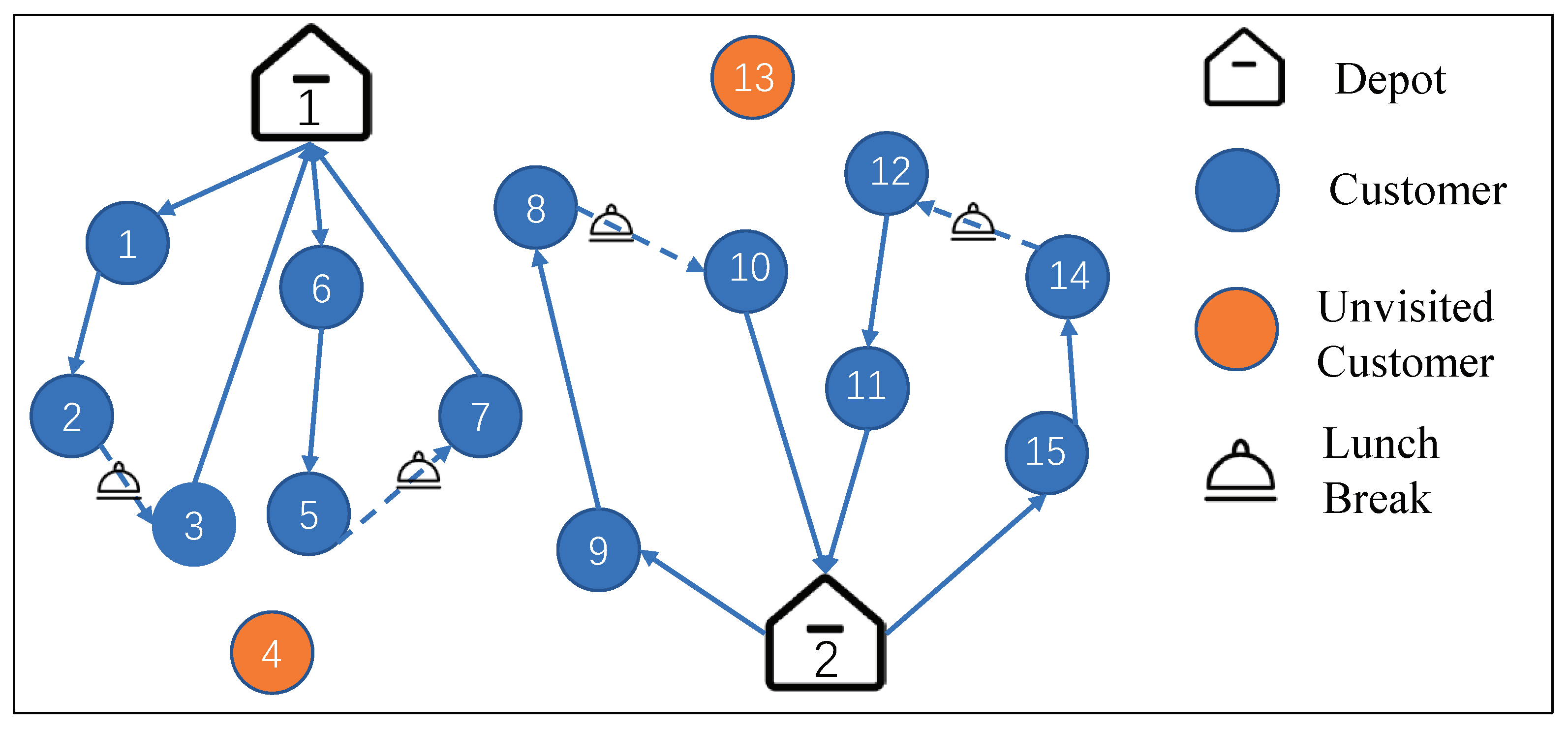
3.1. Problem Description

The problem under consideration is defined by a physical network $\mathcal{G}=(\mathcal{N}\cup \mathcal{H},\mathcal{A}={\displaystyle \underset{h\in \mathcal{H}}{\cup }}{\mathcal{A}}_h)$. Each depot has a set of technicians living close to it, and each technician has different levels of proficiency in different areas of skill. We make the following assumptions to facilitate problem modeling.

• Each customer requires $\delta$ technicians in certain skill areas with different levels of proficiency, and the technicians from the same depot can form technician groups to serve the customers.
• The comprehensive qualifications of the members of a technician group assigned to a customer must meet the skill requirements of the customer, and assigning “overqualified” groups is permitted at no additional cost. In what follows, we refer to the qualification combination of the members of a technician group as the group qualification of the group.
• A technician group is allowed to arrive at the location of customer i before $e_i$ and wait until the customer becomes available, and arrival after $d_i$ is permitted at an additional penalty cost depending on how late it is. However, the maximum lateness is limited, i.e., the service start time at customer i cannot be later than a threshold $D_i$.
• A lunch break is needed in the planning horizon, which can be scheduled at any time within a predefined time interval. The services for customers cannot be interrupted by lunch breaks.
• If the technician groups cannot provide a service to a certain customer due to the capacity limit, the customer can be outsourced at an additional outsourcing cost.
• Traversing each arc incurs a fixed travel cost.

The route of a technician group belonging to the depot $h\in \mathcal{H}$ is a walk $r=(r_0,r_1,\dots ,$$r_p,r_{p+1})$ with a time vector $(T_1,\dots ,T_{p+1})$, where $r_0=h_o$ and $r_{p+1}=h_d$ denote the start and end depots of the route, respectively; $r_q\in \mathcal{N},q=1,\dots ,p$, and $T_q,q=1,\dots ,p+1$, stand for the service start time at customer $r_q$, and all technician groups departing from their depots at time zero. Route r is said to be feasible if $T_{p+1}\le C$ and the service at each customer i visited in the route starts within the time window $[e_i,D_i]$. The STW violation cost for customer $r_q$ is defined as follows:

$$\pi \left(T_q\right)=\left\{\begin{array}{cc}0\hfill & \mathrm{if}{e}_{r_q}\le T_q\le d_{r_q},\hfill \\ {\beta }_{r_q}(T_q-d_{r_q})\hfill & \mathrm{if}{d}_{r_q}<T_q\le D_{r_q},\hfill \\ +\infty \hfill & \mathrm{if}{D}_{r_q}<T_q.\hfill \end{array}\right.$$

The cost of the route r consisting of the travel cost and STW violation cost is defined as follows:

$$c_r=\sum _{q=1}^{p+1}{c}_{r_{q-1},r_q}+\sum _{q=1}^p{\beta }_{r_q}max\{T_q-d_{r_q},0\}.$$

The goal of the problem is to determine the optimal (i) partition of technicians into technician groups; (ii) assignment of technician groups to the customers by considering the compatibility between the group qualifications and customers; (iii) the service route of each technician group; and (iv) setting of the lunch break for each technician group such that each customer is visited by exactly one route or is outsourced, and that the sum of the travel cost, STW violation cost, and outsourcing cost is minimized.

Figure 1 describes a feasible solution for an instance with 2 depots and 15 customers, in which customers 1–3 and 5–7 are served by two technician groups from depot 1, customers 8–12 and 14–15 are served by two technician groups from depot 2, whereas customers 4 and 13 are outsourced due to limited service capacity.

3.2. Model Formulation

With the notation listed in Table 1, the problem can be expressed as a mixed integer linear programming model, to which we refer as $MILP$, as follows.

Minimize ${\displaystyle {\displaystyle \sum _{h\in \mathcal{H}}}}{\displaystyle \sum _{\tau \in {\Gamma }_h}}{\displaystyle \sum _{(i,j)\in {\mathcal{A}}_h}}{c}_{ij}{x}_{ij\tau }^h+{\displaystyle \sum _{h\in \mathcal{H}}}{\displaystyle \sum _{\tau \in {\Gamma }_h}}{\displaystyle \sum _{i\in \mathcal{N}}}{\beta }_i{W}_{i\tau }^h+{\displaystyle \sum _{i\in \mathcal{N}}}{o}_i(1-{\displaystyle \sum _{h\in \mathcal{H}}}{\displaystyle \sum _{\tau \in {\Gamma }_h}}{\displaystyle \sum _{j\in \mathcal{N}\cup \left\{h_d\right\}}}{x}_{ij\tau }^h)$

Subject to the following constraints:

(1a) ${\displaystyle \sum _{h\in \mathcal{H}}}{\displaystyle \sum _{\tau \in {\Gamma }_h}}{\displaystyle \sum _{j\in \mathcal{N}\cup \left\{h_d\right\}}}{x}_{ij\tau }^h\le 1$, $\forall i\in \mathcal{N}$,

(2a) ${\displaystyle \sum _{i\in \mathcal{N}\cup \left\{h_o\right\}}}{x}_{i{h}_d\tau }^h={\displaystyle \sum _{j\in \mathcal{N}\cup \left\{h_d\right\}}}{x}_{h_{o}j\tau }^h\le 1$, $\forall h\in \mathcal{H},\tau \in {\Gamma }_h$,

(3a) ${\displaystyle \sum _{j\in \mathcal{N}\cup \left\{h_d\right\}}}{x}_{ij\tau }^h-{\displaystyle \sum _{j\in \mathcal{N}\cup \left\{h_o\right\}}}{x}_{ji\tau }^h=0$, $\forall i\in \mathcal{N},h\in \mathcal{H},\tau \in {\Gamma }_h$,

(4a) ${\displaystyle \sum _{i\in \mathcal{N}\cup \left\{h_d\right\}}}{v}_{i\tau }^h={\displaystyle \sum _{j\in \mathcal{N}\cup \left\{h_d\right\}}}{x}_{h_{o}j\tau }^h$, $\forall h\in \mathcal{H},\tau \in {\Gamma }_h$,

(5a) $v_{i\tau }^h\le {\displaystyle \sum _{j\in \mathcal{N}\cup \left\{h_o\right\}}}{x}_{ji\tau }^h$, $\forall h\in \mathcal{H},i\in \mathcal{N}\cup \left\{h_d\right\},\tau \in {\Gamma }_h$,

(6a) $T_{i\tau }^h+(t_{ij}+s_i)x_{ij\tau }^h\le T_{j\tau }^h+(1-x_{ij\tau }^h)D_i$, $\forall h\in \mathcal{H},(i,j)\in {\mathcal{A}}_h,\tau \in {\Gamma }_h$,

(7a) $T{b}_{\tau }^h+lb{v}_{j\tau }^h\le T_{j\tau }^h+(1-v_{j\tau }^h)d_b$, $\forall h\in \mathcal{H},j\in \mathcal{N}\cup \left\{h_d\right\},\tau \in {\Gamma }_h$,

(8a) $T_{i\tau }^h+(t_{ij}+s_i+lb)(x_{ij\tau }^h+v_{j\tau }^h-1)\le T_{j\tau }^h+(2-x_{ij\tau }^h-v_{j\tau }^h)D_i$, $\forall h\in \mathcal{H},(i,j)\in {\mathcal{A}}_h,\tau \in {\Gamma }_h$,

(9a) $T_{i\tau }^h+s_i(x_{ij\tau }^h+v_{j\tau }^h-1)\le T{b}_{\tau }^h+(2-x_{ij\tau }^h-v_{j\tau }^h)D_i$, $\forall h\in \mathcal{H},(i,j)\in {\mathcal{A}}_h,\tau \in {\Gamma }_h$,

(10a) $e_i{\displaystyle \sum _{j\in \mathcal{N}\cup \left\{h_o\right\}}}{x}_{ji\tau }^h\le T_{i\tau }^h\le D_i{\displaystyle \sum _{j\in \mathcal{N}\cup \left\{h_o\right\}}}{x}_{ji\tau }^h$, $\forall h\in \mathcal{H},i\in \mathcal{N}\cup \left\{h_d\right\},\tau \in {\Gamma }_h$,

(11a) $e_b{\displaystyle \sum _{i\in \mathcal{N}\cup \left\{h_d\right\}}}{v}_{i\tau }^h\le T{b}_{\tau }^h\le d_b{\displaystyle \sum _{i\in \mathcal{N}\cup \left\{h_d\right\}}}{v}_{i\tau }^h$, $h\in \mathcal{H},\tau \in {\Gamma }_h$,

(12a) $T_{h_d\tau }^h\le C$, $h\in \mathcal{H},\tau \in {\Gamma }_h$,

(13a) ${\displaystyle \sum _{\tau \in {\Gamma }_h}}{u}_{m\tau }^h\le 1$, $\forall h\in \mathcal{H},m\in {\mathcal{M}}_h$,

(14a) $p_{idl}{\displaystyle \sum _{j\in \mathcal{N}\cup \left\{h_d\right\}}}{x}_{ij\tau }^h\le {\displaystyle \sum _{m\in {\mathcal{M}}_h}}{\displaystyle \sum _{l^{\prime }\in \mathcal{L},l\le l^{\prime }}}{q}_{md{l}^{\prime }}{u}_{m\tau }^h$, $\forall d\in \mathcal{D},l\in \mathcal{L},i\in \mathcal{N},h\in \mathcal{H},\tau \in {\Gamma }_h$,

(15a) $T_{i\tau }^h-d_i\le W_{i\tau }^h+(1-{\displaystyle \sum _{j\in \mathcal{N}\cup \left\{h_d\right\}}}{x}_{ij\tau }^h)D_i$, $\forall i\in \mathcal{N},h\in \mathcal{H},\tau \in {\Gamma }_h$,

(16a) $x_{jk\tau }^h,u_{m\tau }^h,v_{i\tau }^h\in \{0,1\}$, $\forall h\in \mathcal{H},(j,k)\in {\mathcal{A}}_h,i\in \mathcal{N}\cup \left\{h_d\right\},m\in {\mathcal{M}}_h,\tau \in {\Gamma }_h$; $T_{j\tau }^h,T{b}_{\tau }^h,W_{i\tau }^h\ge 0$, $\forall h\in \mathcal{H},i\in \mathcal{N},j\in \mathcal{N}\cup \{h_o,h_d\},\tau \in {\Gamma }_h$.

The objective function minimizes the sum of the travel, STW violation, and outsourcing costs. Constraint set (1a) ensures that each customer can be served by at most one technician group. Constraint sets (2a) and (3a) guarantee that if a customer has been assigned to a technician group, this group must enter and leave the customer’s location and depart from the depot and return to it at the end. Constraint set (4a) ensures that each assigned technician group needs to take a break in its route, and constraint set (5a) guarantees that a technician group can take a break before the service at a customer only if the group serves this customer. Constraint set (6a) defines the service start time for each customer. Constraint sets (7a) to (9a) impose the constraints on the time of the lunch break and its adjacent customers. Constraint sets (10a) to (12a) define the time windows of the customers, lunch breaks and technician groups, respectively. Constraint set (13a) guarantees that a technician belongs to one technician group at most in the optimal solution. Constraint set (14a) ensures that a customer can only be assigned to a technician group whose group qualification must meet the skill requirements of the customer. Constraint set (15a) defines the service delay. Finally, constraint set (16a) defines the feasible values for decision variables.

In general, for each $h\in \mathcal{H}$, we assume that $s_{h_o}=s_{h_d}=e_{h_o}=D_{h_o}=d_{h_o}=e_{h_d}=0$ and $D_{h_d}=d_{h_d}=C$, representing the earliest departure time, and latest return time for each technician group. In what follows, let $\mathbf{x}={\left(x_{ij\tau }^h\right)}_{h\in \mathcal{H},(i,j)\in {\mathcal{A}}_h,\tau \in {\Gamma }_h}$, $\mathbf{u}={\left(u_{m\tau }^h\right)}_{h\in \mathcal{H},m\in {\mathcal{M}}_h,\tau \in {\Gamma }_h}$, $\mathbf{v}={\left(v_{i\tau }^h\right)}_{h\in \mathcal{H},i\in \mathcal{N}\cup \left\{d_h\right\},\tau \in {\Gamma }_h}$ and $\mathbf{T}={\left(T_{i\tau }^h\right)}_{h\in \mathcal{H},i\in \mathcal{N}\cup \left\{d_h\right\},\tau \in {\Gamma }_h}$, and denote by $(\mathbf{x},\mathbf{u},\mathbf{v},\mathbf{T})$ a feasible solution to the $MILP$. It is noteworthy that the problem under consideration contains the vehicle routing problem with time windows as a special case, which has been shown to be $NP$-hard in the strong sense even for finding a feasible solution (Solomon [37], Solomon and Desrosiers [38]), implying that it cannot be expected to use exact methods to solve large-scale instances. Therefore, we present a Lagrangian heuristic for its resolution, which is presented in the next section.

4. Lagrangian Relaxation

The Lagrangian heuristic is an optimization method that efficiently finds approximate solutions by decomposing the original problem into several subproblems by relaxing some constraints, referred to as Lagrangian relaxation. Furthermore, the structure of $MILP$ makes it amenable to Lagrangian relaxation. To exploit such a structure, constraint set (1a), referred to as the set of linkage constraints, is relaxed and dualized in the objective function with a nonnegative vector $\mu ={\left({\mu }_i\right)}_{i\in \mathcal{N}}$ of Lagrangian multipliers. The problem resulting from Lagrangian relaxation, referred to as the Lagrangian sub-problem, is

(1b) $L\left(\mu \right)=min{\displaystyle \sum _{h\in \mathcal{H}}}{\displaystyle \sum _{\tau \in {\Gamma }_h}}{\displaystyle \sum _{(i,j)\in {\mathcal{A}}_h}}{c}_{ij}{x}_{ij\tau }^h+{\displaystyle \sum _{h\in \mathcal{H}}}{\displaystyle \sum _{\tau \in {\Gamma }_h}}{\displaystyle \sum _{i\in \mathcal{N}}}{\beta }_i{W}_{i\tau }^h+{\displaystyle \sum _{i\in \mathcal{N}}}{o}_i-$

${\displaystyle \sum _{i\in \mathcal{N}}}{\displaystyle \sum _{h\in \mathcal{H}}}{\displaystyle \sum _{\tau \in {\Gamma }_h}}{\displaystyle \sum _{(i,j)\in {\mathcal{A}}_h}}{o}_i{x}_{ij\tau }^h+{\displaystyle \sum _{i\in \mathcal{N}}}{\mu }_i\left({\displaystyle \sum _{h\in \mathcal{H}}}{\displaystyle \sum _{\tau \in {\Gamma }_h}}{\displaystyle \sum _{(i,j)\in {\mathcal{A}}_h}}{x}_{ij\tau }^h-1\right)$

$=min{\displaystyle \sum _{h\in \mathcal{H}}}{\displaystyle \sum _{\tau \in {\Gamma }_h}}{\displaystyle \sum _{(i,j)\in \mathcal{A}}}(c_{ij}+({\mu }_i+{\mu }_j)/2-(o_i+o_j)/2)x_{ij\tau }^h+{\displaystyle \sum _{h\in \mathcal{H}}}{\displaystyle \sum _{\tau \in {\Gamma }_h}}{\displaystyle \sum _{i\in \mathcal{N}}}{\beta }_i{W}_{i\tau }^h$

$+{\displaystyle \sum _{i\in \mathcal{N}}}(o_i-{\mu }_i)$,

subject to the constraint sets (2a)–(16a).

4.1. Bidirectional Labeling Algorithm for the Lagrangian Sub-Problem

Because the group size and technician composition are predefined, as in Zamorano and Stolletz [12], it can be assumed that all possible technician groups are known in advance. To be precise, we check whether the qualification of a technician group $\tau \in {\Gamma }_h$, $h\in \mathcal{H}$ with $|{\Gamma }_h|=\frac{|{\mathcal{M}}_h|}{\delta !\left(\right|{\mathcal{M}}_h|-\delta )!}$, satisfies some requests’ service requirement; if not, we delete $\tau$ from ${\Gamma }_h$. In addition, for the technician groups with the same qualification in ${\Gamma }_h$, we delete the redundant ones to ensure that each technician is assigned to at most one such group. We denote by ${\overline{\Gamma }}_h,h\in \mathcal{H},$ the resulting groups from depot h. Thus, technicians are partitioned into possible groups and can be pre-defined in the above manner.

We assume that there are $b_h$ different group qualifications in depot $h\in \mathcal{H}$, and let ${\Xi }^h=\{{\Phi }_1^h,\dots ,{\Phi }_{b_h}^h\}$ be the set of different group qualifications, and that there are $b_p^h,p=1,\dots ,b_h$, groups that have the group qualification ${\Phi }_p^h$. Thus, $\sum _{q=1}^{b_h}{b}_q^h=\left|{\overline{\Gamma }}_h\right|$. Let ${\mathcal{N}}_{(h,{\Phi }_p^h)}$ be the set of customers that can be served by the technician groups with group qualification ${\Phi }_p^h$ and ${\mathcal{A}}_{(h,{\Phi }_p^h)}=\{(i,j)\in {\mathcal{A}}_h|i\in {\mathcal{N}}_{(h,{\Phi }_p^h)}\cup \left\{h_o\right\},j\in {\mathcal{N}}_{(h,{\Phi }_p^h)}\cup \left\{h_d\right\},i\ne j\}$ be the corresponding arc set. Using the above notation, the Lagrangian sub-problem can be reformulated as

(1c) $L\left(\mu \right)=min{\displaystyle \sum _{h\in \mathcal{H}}}{\displaystyle \sum _{{\Phi }_p^h\in {\Xi }^h}}{b}_p^h{L}_{(h,{\Phi }_p^h)}\left(\mu \right)+{\displaystyle \sum _{i\in \mathcal{N}}}(o_i-{\mu }_i)$,

in which $L_{(h,{\Phi }_p^h)}\left(\mu \right)$ is defined as follows:

(2c) $L_{(h,{\Phi }_p^h)}\left(\mu \right)=min{\displaystyle \sum _{(i,j)\in {\mathcal{A}}_{(h,{\Phi }_p^h)}}}(c_{ij}+({\mu }_i+{\mu }_j)/2-(o_i+o_j)/2)x_{ij\tau }+{\displaystyle \sum _{i\in {\mathcal{N}}_{(h,{\Phi }_p^h)}}}{\beta }_i{W}_{i,{\Phi }_p^h}$,

subject to the constraint sets (2a)-(11a) and (14a)-(16a), in which $W_{i,{\Phi }_p^h}$ denotes the STW violation cost at customer i in the route of the technician group with group qualification ${\Phi }_p^h$.

Given $h\in \mathcal{H}$, ${\Phi }_p^h\in {\Xi }_h^d$ and the Lagrangian multiplier vector $\mu$, we refer to the problem of exactly computing $L_{(h,{\Phi }_p^h)}\left(\mu \right)$ as $LS{P}_{(h,{\Phi }_p^h)}\left(\mu \right)$, which is concerned with finding feasible routes in the physical subnetwork $({\mathcal{N}}_{(h,{\Phi }_p^h)}\cup \{h_o,h_d\},{\mathcal{A}}_{(h,{\Phi }_p^h)})$ such that the operational cost is calculated according to Eq. (2c) is minimized. In the following, we devise a dynamic programming-based (DP-based) bidirectional labeling algorithm to solve $LS{P}_{(h,{\Phi }_p^h)}\left(\mu \right)$, i.e., by propagating labels forward and backward from $o_h$ and $d_h$, respectively. The DP-based bidirectional labeling algorithm was first developed by Righini and Salani [39,40] for the resource constrained elementary shortest route problem, and it has been shown that it can significantly improve the computing time of the algorithm compared to a unidirectional procedure. In the subsequent sections, we first describe the forward and backward label structures. Second, we elaborate on the label extensions and the dominance procedure we apply. Finally, we develop a method for merging the forward and backward labels.

4.1.1. Label Structure

In the DP-based bidirectional labeling algorithm, each vertex of the physical subnetwork is associated with several forward and backward states. A forward label corresponding to vertex $i\in {\mathcal{N}}_{(h,{\Phi }_p^h)}\cup \left\{h_o\right\}$ encodes a feasible route of served customers from $h_o$ to i. Each vertex generally corresponds to several labels since multiple feasible routes can end at that vertex.

To be precise, a forward label corresponding to vertex $i\in {\mathcal{N}}_{(h,{\Phi }_p^h)}\cup \left\{h_o\right\}$ is represented by $L_i^{fw}=(t^{fw},a^{fw},g^{fw},c^{fw},i)$ with the following semantics:

(1d) i: last served customer;

(2d) $t^{fw}$: service start time for customer i;

(3d) $a^{fw}$: a binary variable equal to 1 if and only if the technician group has taken a break before providing the service to customer i;

(4d) $g^{fw}=(g^{fw}\left[k\right]:k\in {\mathcal{N}}_{(h,{\Phi }_p^h)})$: a $|{\mathcal{N}}_{(h,{\Phi }_p^h)}|$ dimensional binary vector, in which $g^{fw}\left[k\right]$ is equal to 1 if and only if customer k has already been served on the partial route associated with the label or if this route cannot be feasibly extended to customer k because the STW constraint and closing time constraint;

(5d) $c^{fw}$: cost of the partial route calculated according to Equation (2c).

A backward label corresponding to vertex $i\in {\mathcal{N}}_{(h,{\Phi }_p^h)}\cup \left\{h_d\right\}$ is represented by $L_i^{bw}=(t^{bw},a^{bw},g^{bw},c^{bw},i)$, which encodes a feasible route of served customers from i to $h_d$, where $a^{fw},g^{fw}$ and $c^{fw}$ are defined as analogous to those in the forward label, and $t^{bw}$ is the departure time from i.

4.1.2. Propagation

The DP-based bidirectional labeling algorithm iteratively propagates all the feasible forward and backward labels to form new labels. The propagation of a forward label corresponding to vertex i means that appending an additional arc $(i,j)$ to a route from $h_o$ to i, resulting in a route from $h_o$ to j. In a similar way, the propagation of a backward label corresponding to vertex i indicates that appending an additional arc $(j,i)$ to a route from i to $h_d$, resulting in a route from j to $h_d$.

In forward propagation, the label at $h_o$ is initialized as $(0,0,\mathbf{0},0,h_o)$. The search is restricted to elementary propagations to any node j such that $g^{fw}\left[j\right]=0$. When a label $L_i^{fw}=(t^{fw},a^{fw},g^{fw},c^{fw},i)$ is propagated along arc $(i,j)$, two cases are considered.

Case F1. No lunch break occurs when the label propagates along the arc $(i,j)$. In this case, a new label $L_j^{fw}=(g^{\prime fw},t^{\prime fw},a^{\prime fw},c^{\prime fw},j)$ is generated, in which

(1e) $t^{\prime fw}=max\{t^{fw}+s_i+t_{ij},e_j\},$

(2e) $a^{\prime fw}=a^{fw},$

(3e) $g^{\prime fw}\left[k\right]=\left\{\begin{array}{cc}1\hfill & \mathrm{if}k=j\mathrm{or}(k\ne j,t^{\prime fw}+s_j+t_{jk}>D_k,\hfill \\ & \mathrm{and}max\{t^{\prime fw}+s_j+t_{jk},e_k\}+s_k+t_{k{d}_h}>C),\hfill \\ g^{fw}\left[k\right]\hfill & \mathrm{otherwise},\hfill \end{array}\right.,\forall k\in {\mathcal{N}}_{(h,{\Phi }_p^h)},$

(4e) $c^{\prime fw}=c^{fw}+c_{ij}+({\mu }_i+{\mu }_j)/2-(o_i+o_j)/2+{\beta }_{j}max\{t^{\prime fw}-d_j,0\}$.

Case F2. A lunch break is taken when the label propagates along arc $(i,j)$, i.e., the technician group will have lunch before the start of the service for customer j and after departure from vertex i. This case indicates that a lunch break cannot be taken before serving customer i. Thus, there must be $a^{fw}=0$. Moreover, to respect the time window constraint of the lunch break, STW constraint of customer j and closing time constraint, the following constraints should be satisfied: $t^{fw}+s_i\le d_b$, $max\{t^{fw}+s_i+t_{ij},e_b\}+lb\le D_j$, and $max\{max\{t^{fw}+s_i+t_{ij},e_b\}+lb,e_j\}+s_j+t_{j{h}_d}\le C$, respectively. Under the above conditions, a new label $L_j^{fw}=(t^{″fw},a^{″fw},g^{″fw},c^{″fw},j)$ is generated, in which

(5e) $t^{\prime \prime fw}=max\{max\{t^{fw}+s_i+t_{ij},e_b\}+lb,e_j\},$

(6e) $a^{\prime \prime fw}=1,$

and $g^{\prime \prime fw}\left[k\right]$ and $c^{″fw}$ are updated as those in $g^{\prime fw}\left[k\right]$ and $c^{\prime fw}$, respectively.

The label generating rules and feasibility tests for backward propagation are symmetrical. Backward propagation starts at time C denoting the latest possible arrival time at $h_d$. The label at $h_d$ is initialized as $(C,0,\mathbf{0},0,h_d)$. The search is restricted to elementary backward propagation to any node j such that $g^{bw}\left[j\right]=0$. When a label $L_i^{bw}=(t^{bw},a^{bw},g^{bw},c^{bw},i)$ is propagated along arc $(j,i)$, two cases are considered.

Case B1. No lunch break occurs when the label propagates along the arc $(j,i)$. In this case, a new label $L_j^{bw}=(t^{\prime bw},a^{\prime bw},g^{\prime bw},c^{\prime bw},j)$ is generated, in which

(7e) $t^{\prime bw}=min\{t^{bw}-s_i-t_{ji},D_j+s_j\},$

(8e) $a^{\prime bw}=a^{bw},$

(9e) $g^{\prime bw}\left[k\right]=\left\{\begin{array}{cc}1\hfill & \mathrm{if}k=j\mathrm{or}(k\ne j,t^{\prime bw}-s_j-t_{kj}<e_k+s_k\hfill \\ & \mathrm{and}min\{t^{\prime bw}-s_j-t_{kj},D_k+s_k\}-s_k-t_{h_{o}k}<0),\hfill \\ g^{bw}\left[k\right]\hfill & \mathrm{otherwise},\hfill \end{array}\right.,\forall k\in {\mathcal{N}}_{(h,{\Phi }_p^h)},$

(10e) $c^{\prime bw}=c^{bw}+c_{ji}+({\mu }_i+{\mu }_j)/2-(o_i+o_j)/2+{\beta }_{j}max\{t^{\prime bw}-s_j-d_j,0\}$.

Case B2. A lunch break occurs when the label propagates along arc $(j,i)$. This case indicates that a lunch break cannot be taken before serving customer i, and thus there must be $a^{bw}=0$. Moreover, in this case, to respect the time window constraint of the lunch break, STW constraint of customer j and opening time of the depot, the following constraints should be satisfied: $t^{bw}-s_i\ge e_b+lb$, $min\{t^{bw}-s_i-t_{ij},d_b\}-lb\ge e_j+s_j$, and $min\{min\{t^{bw}-s_i-t_{ij},d_b\}-lb,D_j+s_j\}-s_j-t_{h_{o}j}\ge 0$. Under the above conditions, a new label $L_j^{bw}=(g^{″bw},t^{″bw},a^{″bw},c^{″bw},j)$ is generated, in which

(11e) $t^{\prime \prime bw}=min\{min\{t^{bw}-s_i-t_{ij},d_b\}-lb,D_j+s_j\},$

(12e) $a^{\prime \prime bw}=1,$

and $g^{\prime \prime bw}\left[k\right]$ and $c^{″bw}$ are updated as those in $g^{\prime bw}\left[k\right]$ and $c^{\prime bw}$, respectively.

4.1.3. Dominance Test

In the above propagation procedure, all possible propagations for each label are generated and stored, resulting in a large number of labels. Thus, it is critical to abandon labels, which cannot lead to a complete optimal route. To reduce the number of labels, a dominance test is needed. Let $L_i=(t,a,g,c,i)$ and $L_i^{\prime }=(t^{\prime },a^{\prime },g^{\prime },c^{\prime },i)$ be two labels corresponding to the vertex i. Then, label $L_i$ dominates label $L_i^{\prime }$ if:

(1f) $g\left[k\right]\le g^{\prime }\left[k\right],\forall k\in {\mathcal{N}}_{(h,{\Phi }_p^h)},$

(2f) $t\le t^{\prime }$ for forward labels and $t\ge t^{\prime }$ for backward labels,

(3f) $a\ge a^{\prime },$

(4f) $c\le c^{\prime },$

and at least one of the inequalities is strict true. A label can be abandoned if it is dominated by another label.

4.1.4. Concatenate

In the DP-based bidirectional labeling algorithm, both the forward and backward labels are not necessarily propagated until $h_o$ and $h_d$, respectively. Instead, the labels are propagated only up to a predefined halfway point, thereby reducing the total number of generated labels. Suitable forward and backward labels are then concatenated to generate complete routes. In our DP-based bidirectional labeling algorithm, we only propagate the forward labels whose service start times are less than $C/2$ and the backward labels whose departure times are larger than $C/2$, i.e., $t^{fw}<C/2$ and $t^{bw}>C/2$. A forward label $L_i^{fw}=(t^{fw},a^{fw},g^{fw},c^{fw},i)$ and a backward label $L_i^{bw}=(t^{bw},a^{bw},g^{bw},c^{bw},i)$ can be concatenated together to generate a complete feasible route if $N\left(L_i^{fw}\right)\cap N\left(L_i^{bw}\right)=\left\{i\right\}$, $a^{fw}+a^{bw}=1$, and $t^{fw}+s_i\le t^{bw}$, where $N\left(L_i^{fw}\right)$ and $N\left(L_j^{bw}\right)$ denote the customers served by the routes corresponding to labels $L_i^{fw}$ and $L_j^{bw}$, respectively.

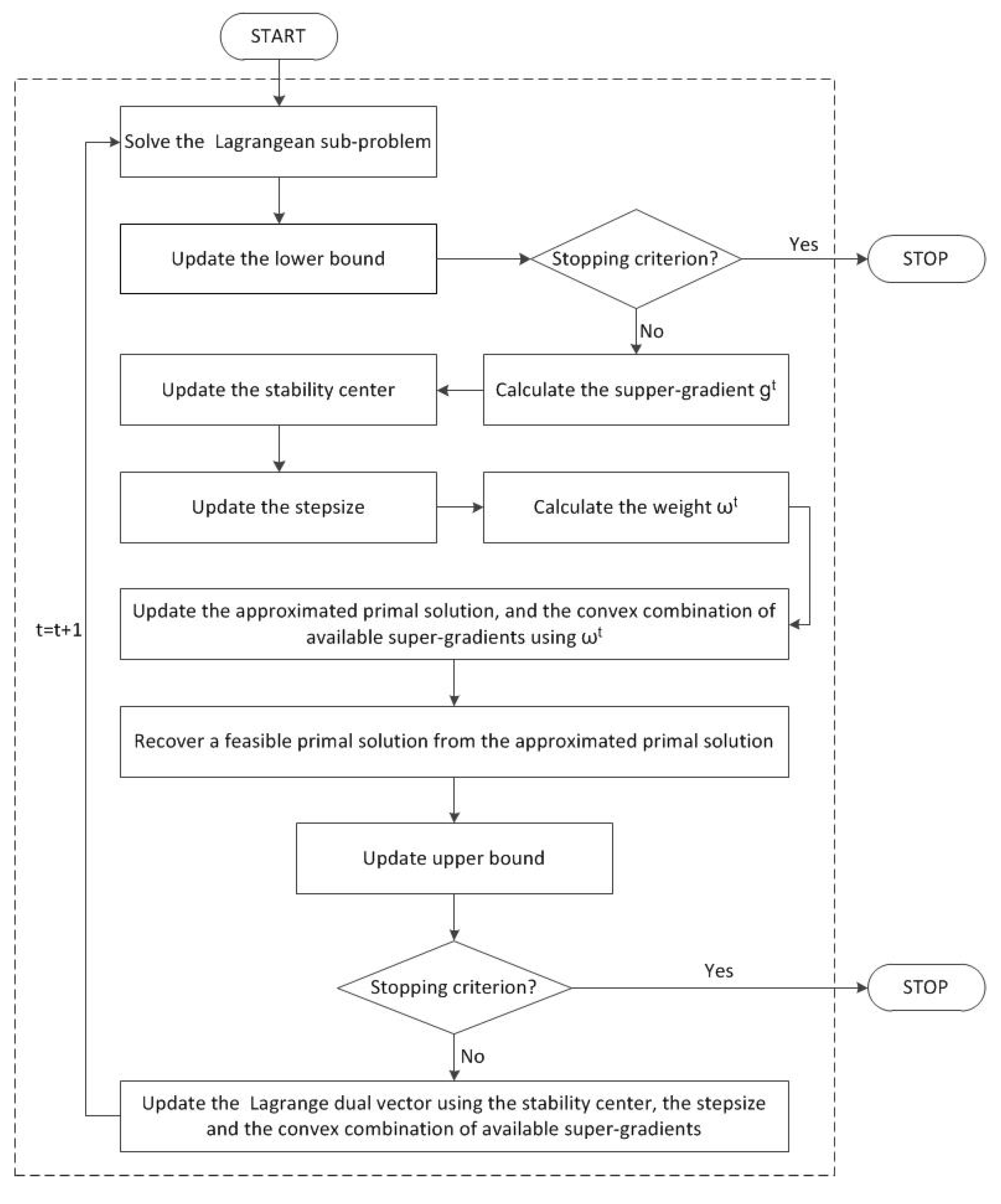
4.2. The Lagrangian Heuristic

The optimal solution of the Lagrangian sub-problem, for any Lagrange multiplier vector $\mu$, yields a lower bound to the problem under consideration. To obtain the best possible lower bound, we must solve the following Lagrangian dual problem

(1g) $z^{*}={\displaystyle \underset{\mu >0}{max}}L\left(\mu \right)$.

The above Lagrangian dual problem is concave and non-differentiable, and is usually solved by non-smooth optimization methods, including the sub-gradient, analytic center, bundle method, or cutting-planes. Indeed, all the aforementioned methods have advantages and disadvantages, the efficiency of which highly depends on the characteristic of the problem to be solved. For example, sub-gradient methods are known for their simplicity, but they are also known for their lack of well-defined stopping conditions and producing values for the primal variables. On the other hand, bundle methods are considered robust and precise, but need to solve a quadratic program in each iteration. To overcome the drawbacks of the sub-gradient method, the volume algorithm was presented by Barahona and Anbil [41] as a subgradient-like method that will produce an approximation to a primal solution and provide much better stopping conditions. In this study, we adopt the revised volume algorithm (RVA) developed by Bahiense et al. [42] with the aim of exploiting the advantages of the sub-gradient and bundle methods. In particular, to obtain a high-quality dual solution, the RVA produces sampling points ${\mu }^t$ by solving a series of Lagrangian sub-problems, in which the calculation of ${\mu }^t$ depends on: (i) a given stability center ${\widehat{\mu }}^p$, which is a special sampling point that provides a “good enough” improvement during the iteration process; (ii) a stepsize $s^t$; and (iii) a convex combination of available super-gradients.

A primal solution can then be expressed as a convex combination of past primal solutions, in which the weights used in such convex combinations are identical to those applied for calculating $d^t$.

Adapting the ideas of the algorithms developed by Bahiense et al. [42], Barahona and Anbil [41], and Frangioni et al. [43], we develop a Lagrangian heuristic, referred to as Algorithm $LBH$, in which the RVA is applied to solve the Lagrangian dual problem, and provide the details of its main components, including the way to produce an initial incumbent to obtain an upper bound, and the way to translate the approximated primal solution obtained during the implementation of the algorithm to a feasible solution in the subsequent subsections. The four stopping criteria are as follows: the maximum number of iterations $MAXITER$, the maximum limit of computing time $MAXITIME$, the relative gap between the lower and upper bounds $\epsilon$, and the ascent measures ${\delta }_e$ and ${\delta }_{ϵ}$. Here, we just provide a flow chart of our implementation of the Lagrangian heuristic in Figure 2, and refer readers to Bahiense et al. [42] for details. The formal pseudocode is depicted in Algorithm $LBH$ in Appendix A.

4.3. Upper-Bound Generation Based on the Lagrangian Solutions

Finding a good upper bound for the problem under consideration is an essential component of Algorithm $LBH$, which is crucial for speeding up the convergence of the algorithm. However, because the binary decision variables involved and the stopping conditions used, approximated primal solution ${\chi }^t$ generated during the implementation of Algorithm $LBH$ is generally infeasible for the original problem, i.e., the binary variables $x_{ij\tau }^h$ might be fractional, and the constraint set (1a) might not hold. To obtain a good feasible solution to the original problem based on ${\chi }^t$, we propose a two-stage hybrid heuristic. The main idea is as follows: after an approximated primal solution ${\chi }^t$ is generated, a feasibility recovery procedure is first applied to recover a feasible solution based on this solution when the conditions in line 32 of Algorithm $LBH$ hold. Using the obtained feasible solution as an initial solution, a TS algorithm is then used to derive a better feasible solution.

4.3.1. A Feasibility Recovery Procedure

The approximated primal solution ${\chi }^t$ provides the schedule assigning customers to the routes of groups or outsourcing them. Because of the iteration rule and the fact that the assignment constraint set (1a) has been relaxed, the binary variables $x_{ij\tau }^h$ might be fractional, and the constraint set (1a) might not hold.

To recover an integer feasible solution based on ${\chi }^t=(\widehat{\mathbf{x}},\widehat{\mathbf{v}})$, we develop a heuristic comprising of two phases.

In the first phase, we derive an integer solution from ${\chi }^t$. To be precise, for each $i\in \mathcal{N}$, the variables in the set ${\displaystyle \underset{h\in \mathcal{H}}{\cup }}{\displaystyle \underset{\tau \in {\Gamma }^h}{\cup }}{\displaystyle \underset{j\in (N\cup \{h\left\}\right)\setminus \left\{i\right\}}{\cup }}\left\{{\widehat{x}}_{ij\tau }^h\right\}$ with a fractional value of no less than 0.8 are fixed at 1, whereas the other fractional variables are fixed at 0.

Let $I_{\tau },h\in \mathcal{H},\tau \in {\overline{\Gamma }}^h,$ be the set of customers served by the group $\tau$ in the current integer solution. A complete solution is then constructed by splicing the partial routes covered by each technician group $\tau ,h\in \mathcal{H},\tau \in {\overline{\Gamma }}^h$, with $I_{\tau }\ne \varnothing$ in the cheapest manner. In the construction process, ${\widehat{x}}_{ij\tau }^h$ is reset to 1 if i and j are the end and start vertices of the partial routes, respectively. In addition, if ${\displaystyle \sum _{h\in \mathcal{H}}}{\displaystyle \sum _{\tau \in {\Gamma }_h}}{\displaystyle \sum _{j\in N\cup \left\{h\right\}}}{\widehat{x}}_{ij\tau }^h=0$, we then assign customer i into the outsourced customer set.

In the second phase, we translate the solution obtained in the first phase into a feasible integer solution. As the assignment constraint set (1a) has been relaxed and the construction strategy in the first phase, the assignment of customers to the routes of technician groups are either exactly satisfied (assigned to exactly one route or outsourced) or overassigned. Therefore, the set of all customers can be divided into two disjoint subsets, in which ${\Lambda }_1$ and ${\Lambda }_2$ represent the customers that are exactly satisfied and overassigned, respectively: (i) ${\Lambda }_1=\{i:{\displaystyle \sum _{h\in \mathcal{H}}}{\displaystyle \sum _{\tau \in {\overline{\Gamma }}_h}}{\displaystyle \sum _{j\in N\cup \left\{h\right\}}}{\widehat{x}}_{ij\tau }^h\le 1\}$; and (ii) ${\Lambda }_2=\{i:{\displaystyle \sum _{h\in \mathcal{H}}}{\displaystyle \sum _{\tau \in {\overline{\Gamma }}_h}}{\displaystyle \sum _{j\in N\cup \left\{h\right\}}}{\widehat{x}}_{ij\tau }^h>1\}$.

To obtain a feasible integer solution, we first check whether the number of technicians qualified with proficiency $l\in \mathcal{L}$ of skill $d\in \mathcal{D}$ in each depot $h\in \mathcal{H}$ used in the resulting solution exceeds $m_{hld}$. If that is the case, we delete the redundant routes of the technician groups in each h containing the technicians with proficiency l of skill d in the cheapest way, because each technician can belong to at most one used technician group. We then remove the customers in ${\Lambda }_2$ from the redundant routes left after implementing the first step. To be precise, for each customer $i\in {\Lambda }_2$, we remove it from the routes in the cheapest manner as follows. Let $f_{▽}(i,r)$ denote the reduction in the sum of the travel cost and STW violation cost for removing customer i from route r. We select a route $r^{*}$ such that $r^{*}=arg{\displaystyle \underset{r\in {\mathcal{S}}_i}{min}}{f}_{▽}(i,r)$, in which ${\mathcal{S}}_i$ contains all routes of technician groups that provide service to customer i in the current integer solution. It follows that maintaining customer i in the route $r^{*}$ and deleting it from all routes in ${\mathcal{S}}_i\setminus \left\{r^{*}\right\}$ is the best choice to keep customer i being served.

To determine whether it is better to keep customer i outsourced, we must compare $f_{▽}(i,r^{*})$ and $o_i$. If $f_{▽}(i,r^{*})\le o_i$, we keep customer i in route $r^{*}$ and remove i from all routes in ${\mathcal{S}}_i\setminus \left\{r^{*}\right\}$. Otherwise, we remove customer i from all the routes in ${\mathcal{S}}_i$, and add it to the outsourced customer set.

4.3.2. Upper-Bound Improvement: TS Algorithm

TS algorithm is a meta-heuristic that utilizes a memory scheme to direct the local search to avoid repeated access to the same solutions (Glover and Laguna [44]), which has been successfully applied to solve various vehicle routing problems (see, e.g., Berbeglia et al. [45], Gendreau et al. [46]). In this subsection we develop a TS algorithm by adapting the idea of Archetti [47] to further improve the integer feasible solution $(\overline{\mathbf{x}},\overline{\mathbf{u}},\overline{\mathbf{v}})$ obtained in Algorithm $FR$. The developed TS algorithm depends on two operators: deleting a customer from the outsourced customer set and inserting it into a route, and removing a customer from a route and adding it into the outsourced customer set. Specifically, let $\mathcal{O}$ be the outsourced customer set, $r_{\tau }$ the route of the group $\tau$, and $\mathcal{S}$ the set of all routes of the current solution, and let $N\left(r_{\tau }\right)$ and $N_{\tau }$ be the set of customers served by $r_{\tau }$ and the set of customers that can be served by the technician group $\tau$, respectively. Given a route $r_{\tau }$, the neighborhood of $r_{\tau }$ is determined by the following operators.

(i) Deletion–insertion: Consider customer $i\in \mathcal{O}$, deleting it from $\mathcal{O}$ and inserting it into $r_{\tau }$ at the cheapest possible position. The route derived from this move is denoted as $r_{\tau }+i$.

(ii) Remove–addition: Consider customer $i\in N\left(r_{\tau }\right)$, removing it from $r_{\tau }$ and adding it to $\mathcal{O}$. The route derived from this move is denoted as $r_{\tau }-i$.

5. Computational Results

In this section, we conduct numerical experiments to: (i) qualify the efficiency of Algorithm $TS$ for improving the upper bound in Algorithm $LBH$; (ii) verify the effectiveness of Algorithm $LBH$; and (iii) investigate the impacts of the key model parameters on the solution structure.

The algorithms have been coded in MATLAB. The IBM ILOG CPLEX optimization library version 12.8.0 was used to solve the $MILP$ formulation. All experiments were conducted on a workstation with 8G RAM and an Intel Core i7 3.4 GHz CPU.

5.1. Problem Instances

To assess the performance of the proposed algorithms, we tested instances generated by the following scheme, similar to that described by Kovacs et al. [11]. These instances were generated based on the well-known VRPTW benchmark instances of Solomon [37] and were grouped into six classes. In Classes R1 and R2, customers are randomly distributed in a square region. In Classes C1 and C2, customers are clustered, and in Classes RC1 and RC2, customer distribution is mixed. Associated with R1, C1, and RC1 is a short planning horizon, while associated with instances R2, C2, and RC2 is a long planning horizon implying that each route can visit more customers. Each instance contained 100 customers, and the travel times and costs are equal to the Euclidean distances between the corresponding vertices.

We considered six different sizes of instances: 50 customers with 5 technicians, 60 customers with 7 technicians, 70 customers with 9 technicians, 80 customers with 11 technicians, 90 customers with 13 technicians, and 100 customers with 15 technicians, where 50-, 60-, 70-, 80- and 90-customer instances were generated by considering only the first 50, 60, 70, 80, and 90 customers, respectively. In each instance, two depots were involved. One corresponds to the depot of the Solomon instance, and the coordinates of the other were randomly generated with a uniform probability distribution in the smallest rectangle containing all the customers. The maximum working time of technicians C was set to the latest service start time of the depots. Each customer has a time window $[e_i,d_i]$, and we set $D_i=min\{d_i+ϵ(d_i-e_i),C\}$, in which $ϵ$ was chosen randomly from $\{0.1,0.2,0.3\}$. The time interval $[e_b,d_b]$ for taking a lunch was set to [4C/9,5C/9]. The technicians qualified in two skill domains with three possible proficiency levels, and were paired into teams with size $\delta$ = 2. The qualifications of the technicians and the skill requirements of the customers were randomly generated. In the post-processing step, we adjusted the skill requirement matrices such that each customer can be served by more than one technician group.

Based on preliminary parameter tuning experiments and the best settings identified by other authors (Archetti et al. [47], Bahiense et al. [42]), the parameters used in the algorithms we develop were set as follows: (i) $\lambda =0.1,{\delta }_d={\delta }_{ϵ}=0.0001,\varsigma =0.001,{\iota }^0=1,{\iota }_f=6,{\iota }_p=0.8,$ and ${\iota }_{min}=0.0001$; and (ii) $maxIo=5$, $maxIn=10$, $maxT=100s$, $mTB=5$, and $\theta =1$.

The model cost parameters ${\beta }_i$ and $o_i$, $i\in N$, are associated with the three subgoals. Generally, the time windows are required by the customers; a late service start time might lead to customer’ complaints, which should be avoided; thus, ${\beta }_i$ should be set higher than the coefficient of travel cost, which is set to be 1. In addition, rejecting a customer during the planning period will dramatically reduce customer satisfaction, and thus $o_i$ should be set such that it is always preferable toserve a customer rather than to outsource them. Thus, for each customer $i\in N$, ${\beta }_i$ was set to $1.5\sigma$/min in monetary units and, as in Kovacs et al. [11], $o_i$ was set to $200+{\left({\displaystyle \sum _{d\in \mathcal{D}}}{\displaystyle \sum _{l\in \mathcal{L}}}{p}_{idl}\right)}^{1.5\xi }$, in which constant 200 is based on the geographic characteristics of the instances: the highest single route costs 200, and the second term defines the difficulty of customer i. Here, $\sigma$ and $\xi$, referred to as the tardiness penalty coefficient and outsourcing penalty index, respectively, were set to one in our numerical study, the impacts of which will be discussed in Section 5.4.

5.2. Impact of Algorithm $TS$ for Improving the Upper Bound

First, we conduct experiments to provide insights into the efficiency of Algorithm $TS$ for improving the upper bound in Algorithm $LBH$, and restricted our test to the 50- and 60-customer instances. In particular, Algorithm $LBH$ with and without Algorithm $TS$ for improving the upper bound is been tested, which is stopped either after a maximum of 5000 iterations or after a maximum of one hour of computing time or when the integrality (optimality) gap is lower than 1%, i.e., $MAXITER=5000$, $MAXTIME=3600$ s, and $\epsilon =0.001$.

The computational results are presented in

Table 2. Performance of tabu search algorithm for n = 50 and 60.

			Without Tabu			With Tabu
n	Group	No. Inst	Avg. Gap	Avg. Time	No.1% Gap	Avg. Gap	Avg. Time	No.1% Gap	DT-Gap	DT-Time	DT-No.1
50	R1	12	5.01	1154.32	5	2.18	967.66	9	56.49	16.17	80.00
	C1	9	5.35	973.33	5	4.04	1012.93	5	24.49	−4.07	0.00
	RC1	8	7.79	928.25	2	4.49	996.72	4	42.36	−7.38	100.00
	R2	11	5.68	1480.13	4	2.89	1263.61	7	49.12	14.63	75.00
	C2	8	5.59	1718.62	3	3.24	1501.21	4	42.04	12.65	33.33
	RC2	8	5.57	1806.60	1	3.15	1562.48	4	43.45	13.51	300.00
Total/Weighted average			5.76	1330.73	20	3.24	1198.42	33	43.75	9.94	65.00
60	R1	12	9.35	1675.21	1	4.32	1584.57	4	53.80	5.41	200.00
	C1	9	8.78	1829.32	1	5.15	1673.01	3	41.34	8.54	100.00
	RC1	8	9.22	2223.12	0	5.89	1842.68	3	36.11	17.11	-
	R2	11	8.69	2802.87	0	4.22	2395.97	4	51.43	14.52	-
	C2	8	10.32	2653.79	1	5.24	2794.73	2	49.22	−5.31	100.00
	RC2	8	8.43	3165.47	0	4.31	2938.70	3	48.87	7.16	-
Total/Weighted average			9.12	2352.45	3	4.79	2161.37	19	47.48	8.13	533.33

by the group of instances, where a group contains instances that belong to the same instance class as the same number of customers. The results in Table 1 below “Without tabu” are obtained without Algorithm $TS$ to improve the upper bound, whereas the results below “With tabu” are obtained with Algorithm $TS$ for improving the upper bound. We report, for each group of instances,

(i) Avg. Gap: the Average optimality gap in percentages between the lower bound $LB$ and upper bound $UB$ found by Algorithm $LBH$ encountering up to the current iteration, in which the optimality gap is calculated by $100\times (UB-LB)/UB$;

(ii) No.1% Gap: the number of instances with 1% optimality gap;

(iii) Avg. Time: the Average computing time in seconds;

(iv) DT-Gap: the percentage difference in the optimality gap calculated by 100 × (Avg. Gap(Without tabu)- Avg. Gap(With tabu))/Avg. Gap(Without tabu);

(v) DT-Time: the percentage difference in computing time calculated by 100 × (Avg. Time(Without tabu)- Avg. Time(With tabu))/Avg. Time(Without tabu); and

(vi) DT-No.1: the percentage difference in the total number of instances with a 1% optimality gap calculated by 100 × (No.1% Gap(With tabu)- No.1% Gap(Without tabu))/No.1% Gap(Without tabu).

The computational results summarized in Table 2 clearly state that Algorithm $TS$ contributes to the effectiveness of Algorithm $LBH$ in improving the upper bound. First, Algorithm $TS$ can significantly close the optimality gap. Specifically, when Algorithm $TS$ is applied, the number of instances, with a 1% optimality gap, increased by 65% and 533.33% for the 50- and 60-customer instances, respectively. Second, with average optimality gaps in percentages of 3.24% and 4.79% when Algorithm $TS$ was applied, it closed the average optimality gap with 43.75% and 47.48% for the 50- and 60-customer instances, respectively. Finally, with average computing times of 1198.42 and 1789.74 seconds, applying Algorithm $TS$ requires less computing time, which decreases the computing times, on average by, 9.94% and 8.13% for the 50- and 60-customer instances, respectively. This is primarily because due to the fact that the additional computational burden of applying Algorithm $TS$ to improve the upper bound is compensated by implementing fewer iterations in Algorithm $LBH$.

5.3. Algorithmic Performance

We now compare the lower bound found by Algorithm $LBH$ to the best lower bound obtained by solving the continuous LP relaxation of the $MILP$ and solving the $MILP$ using the state-of-the-art MIP solver CPLEX. We also report our computational results for solving the $MILP$ using CPLEX vs. Algorithm $LBH$.

We test all the 50-, 60-, 70-, 80- and 90-customer instances. As in the previous experiments, an iteration number limit of 5000 and a 1% optimality stopping criterion are applied. However, for the maximum limit of computing time, we set one hour for the 50- and 60-customer instances, two hours for the 70-customer instances, three hours for the 80-customer instances, and five hours for the 90- and 100-customer instances.

The comparison results are summarized in

Table 3. Algorithmic performance comparisons.

			CPLEX			Algorithm LBH
n	Group	No. Inst	Avg. Gap	Avg. Time	No.1% Gap	Avg.LGap	Avg. Gap	Avg. Time	No.1% Gap	DT-Gap	DT-Time
50	R1	12	0.02	398.47	11	−0.18	2.18	967.66	9	99.08	−58.82
	C1	9	0.00	403.26	9	−0.24	4.04	1012.93	5	100.00	−60.18
	RC1	8	0.11	202.00	7	−0.49	4.49	996.72	4	97.55	−79.73
	R2	11	0.23	1098.85	10	−0.89	2.89	1263.61	7	92.04	−13.03
	C2	8	0.46	783.12	6	−1.24	3.24	1501.21	4	85.80	−47.83
	RC2	8	0.35	652.27	6	−1.15	3.15	1562.48	4	88.89	−58.25
Total/Weighted average			0.18	599.95	49	−0.66	3.24	1198.42	33	94.44	−49.93
60	R1	12	1.15	1951.70	8	0.35	4.32	1584.57	4	73.38	23.16
	C1	9	1.53	2492.17	6	0.07	5.15	1673.01	3	70.29	48.96
	RC1	8	1.41	3032.10	5	0.12	5.89	1842.68	3	76.06	64.54
	R2	11	0.98	2573.21	7	0.33	4.22	2395.97	4	76.78	7.39
	C2	8	1.35	2982.59	4	−0.16	5.24	2794.73	2	74.24	6.72
	RC2	8	1.96	3375.38	4	−0.09	4.31	2938.70	3	54.52	14.85
Total/Weighted average			1.36	2665.64	34	0.13	4.79	2161.37	19	71.61	23.33
70	R1	12	3.55	7100.75	2	2.67	2.43	2576.51	8	−46.09	175.59
	C1	9	4.83	6455.67	3	2.31	3.52	3348.30	6	−37.22	92.80
	RC1	8	4.35	5966.12	2	3.46	3.80	3675.16	5	−14.47	62.33
	R2	11	5.09	7035.27	1	2.65	2.30	2913.52	9	−121.30	141.46
	C2	8	4.98	6818.25	2	2.33	4.36	3442.96	4	−14.22	98.03
	RC2	8	6.12	7200.00	0	2.90	2.88	3956.29	5	−112.50	81.98
Total/Weighted average			4.64	6795.95	10	2.71	3.12	3244.59	37	−52.05	109.45
80	R1	12	9.17	10,800.00	0	3.02	3.09	5756.66	6	−196.76	87.60
	C1	9	12.38	10,800.00	0	3.81	3.24	6048.72	5	−282.09	78.55
	RC1	8	16.80	10,800.00	0	3.48	4.49	6468.72	3	−274.16	66.95
	R2	11	11.11	10,800.00	0	3.78	4.02	6003.66	7	−176.36	79.89
	C2	8	13.17	10,800.00	0	3.06	3.71	5442.96	5	−254.98	98.42
	RC2	8	14.73	10,800.00	0	3.23	4.58	7621.31	4	−221.61	41.70
Total/Weighted average			12.52	10,800.00	0	3.40	3.80	6175.40	30	−229.47	74.89
90	R1	12	-	-	-	3.60	3.18	9250.43	7
	C1	9	-	-	-	4.07	4.16	11,097.18	5
	RC1	8	-	-	-	3.18	4.22	10,667.60	4
	R2	11	-	-	-	3.42	3.27	10,412.88	6
	C2	8	-	-	-	3.17	4.24	11,089.12	4
	RC2	8	-	-	-	4.79	4.04	12,462.54	3
Total/Weighted average			-	-	-	3.69	3.78	10,699.56	29
100	R1	12	-	-	-	4.17	4.24	13,577.78	3
	C1	9	-	-	-	5.12	4.88	15,516.60	3
	RC1	8	-	-	-	4.61	5.02	16,590.84	2
	R2	11	-	-	-	4.21	5.12	16,066.54	2
	C2	8	-	-	-	4.79	5.98	15,909.50	2
	RC2	8	-	-	-	5.06	5.33	17,942.38	1
Total/Weighted average			-	-	-	4.61	5.03	15,765.29	13

, which reports the following indicators:

(i) Avg. LGap: the average gap in percentages between the lower bound $LB$ found by Algorithm $LBH$ and the best lower bound $L{B}_{C-LR}$ obtained by solving the continuous LP relaxation of the $MILP$ and solving the $MILP$ using CPLEX encountering up to the current iteration, in which the gap LGap is calculated as $100\times (LB-L{B}_{C-LR})/L{B}_{C-LR}$;

(ii) Avg. Gap: the average optimality gaps in percentages between the lower and upper bounds found by solving the $MILP$ using CPLEX and Algorithm $LBH$, respectively;

(iii) No.1% Gap: the number of instances with a 1% optimality gap has been proven by solving the $MILP$ using CPLEX and Algorithm $LBH$, respectively, in which we only consider the instances for which CPLEX found a feasible solution when solving the $MILP$ using CPLEX;

(iv) Avg. Time: the average computing time in seconds;

(v) DC-Gap: the percentage difference in the optimality gap calculated by 100 × (Avg. Gap(Algorithm $LBP$)- Avg. Gap(CPLEX))/Avg. Gap(Algorithm $LBP$); and

(vi) DT-Gap: the percentage difference in computing time calculated as 100 × (Avg. Time (CPLEX)- Avg. Time (Algorithm $LBP$))/Avg. Time (Algorithm $LBP$),

in which the character “-” is used to indicate an out-of-memory condition.

The lower bound found using Algorithm $LBP$. From the term “Avg. LGap” in Table 2, one can see that the lower bounds found by Algorithm $LBP$ are very close to the optimal solution values and are quite tight compared to the LP relaxation.

With average gaps in percentages between $LB$ and $L{B}_{C-LR}$ of −0.66% and 0.13% for the 50- and 60-customer instances, respectively, we can conclude that the lower bounds found by Algorithm $LBH$ are close to the optimal solution values. This is due to the fact that CPLEX is capable of solving 83 of the 112 instances to optimality and the average optimality gaps (Avg. Gap(CPLEX)) were only 0.35% and 1.96%, respectively, implying that the obtained $L{B}_{C-LR}$ values were extremely close to the optimal solution values.

With average gaps in percentages between $LB$ and $L{B}_{C-LR}$ of 2.71%, 3.40%, 3.69% and 4.61%, respectively, when the number of customers n ranges from 70 to 100, we can conclude that the lower bounds found by Algorithm $LBH$ are quite tight compared to the LP relaxation. In fact, according to the definition of LGap, the aforementioned data demonstrate that the lower bounds found by Algorithm $LBP$ are at least 0.0271, 0.0240, 0.0369, and 0.0461 times larger on average than the lower bounds found by LP relaxation for the 70-, 80-, 90- and 100-customer instances, respectively. In general, the average gap between $LB$ and $L{B}_{C-LR}$ increases with the number of customers because the problem becomes more complex.

Comparison with CPLEX. The computational results presented in Table 2 allow us to draw the following conclusions: (i) the average quality of the solutions found by CPLEX is quite good for instances with fewer customers, whereas the performance of CPLEX deteriorates as the number of customers increases; and (ii) Algorithm $LBH$ provides stable results for all the test problems, and outperforms CPLEX when the number of customers increases.

Although CPLEX is capable of proving a 1% optimality gap for 83 out of the 112 instances with 50 and 60 customers and consumes less computing time compared with Algorithm $LBH$ for the 50-customer instances, Algorithm $LBH$ outperforms CPLEX when the number of customers is equal to or larger than 70, which lowers the average optimality gap and consumes significantly less computing time when compared to CPLEX. For the 70-customer instances, the average optimality gap found by Algorithm $LBH$ is 34.23% lower than that found by CPLEX, and Algorithm $LBH$ is 1.0945 times faster, on average, than CPLEX. For the 80-customer instances, the average optimality gap found by Algorithm $LBH$ is 69.03% lower than that found by CPLEX, and Algorithm $LBH$ is 0.7489 times faster on average than CPLEX. Most importantly, CPLEX cannot prove a 1% optimality gap for any instance with 80 customers, whereas Algorithm $LBH$ can prove a 1% optimality gap for 30 out of the 56 instances. What is more, CPLEX is unable to solve instances with a number of customers equal to or larger than 90 in most cases, owing to the large increase in the number of variables in $MILP$ and limited computation resources. Instead, with Algorithm $LBH$, the problem can be solved using a desktop with limited computation resources and less RAM. This is because of the iterative nature of Lagrangian heuristics, which is also an advantage over the all-at-once algorithms used in CPLEX.

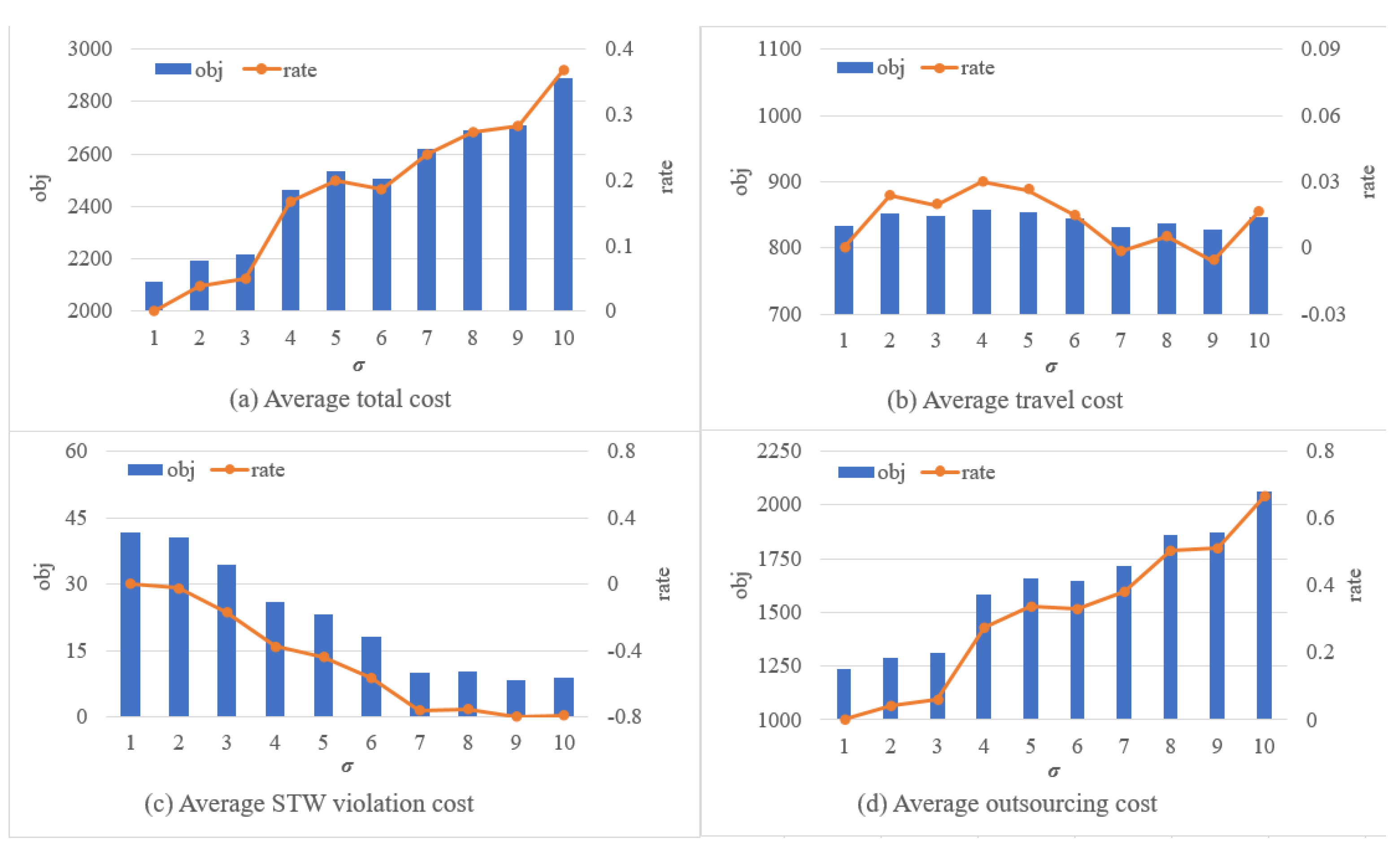
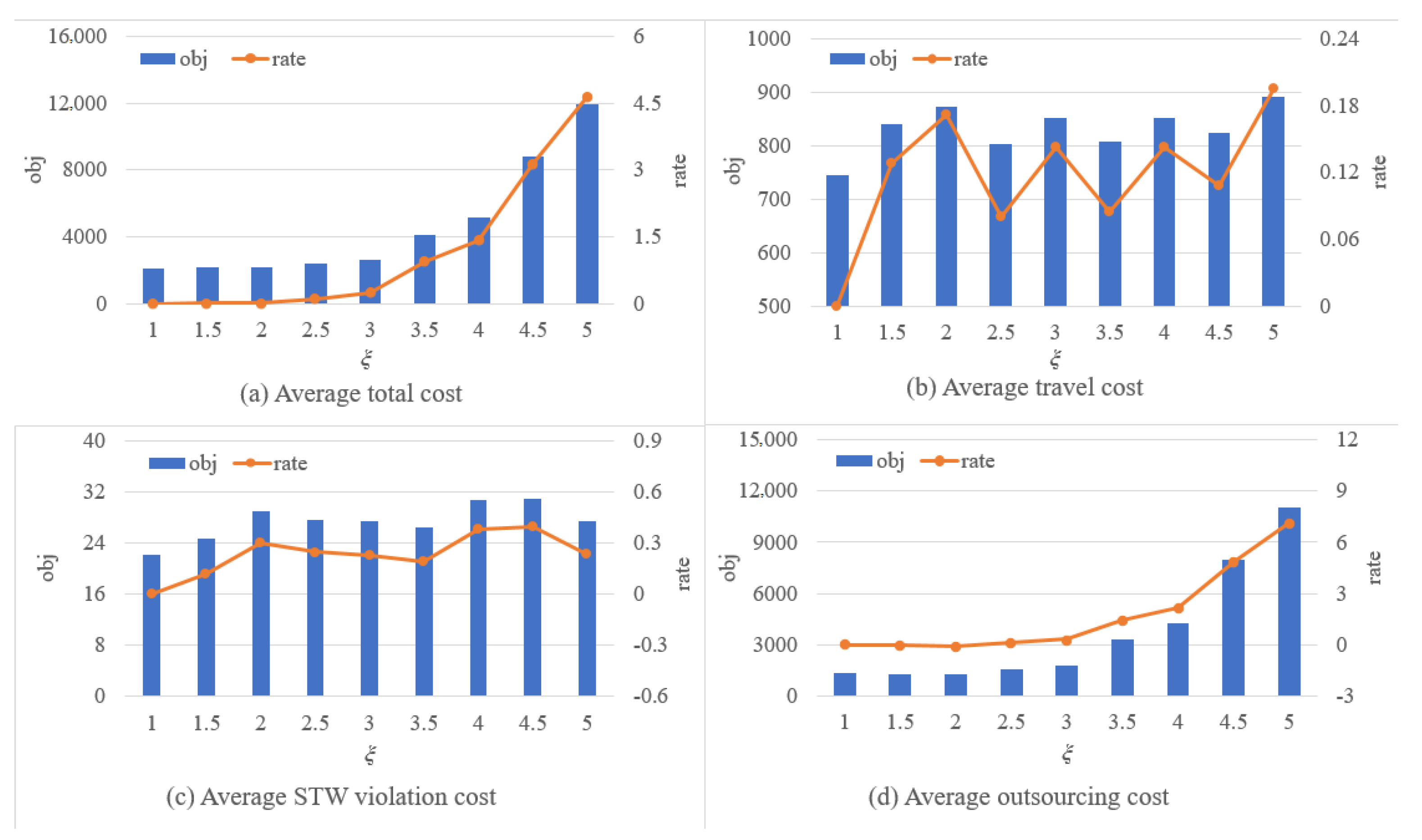
5.4. Sensitivity Analysis

We further investigate the problem we consider in depth by conducting a sensitivity analysis of the solution concerning the tardiness penalty coefficient $\sigma$ and outsourcing penalty index $\xi$ on the 56 instances with $n=60$.

To compare the performance changes, we consider the following four metrics: (i) average total cost, (ii) average travel cost, (iii) average STW violation cost, and (iv) average outsourcing cost. Here, we use the instances that can find the solution with a 1% optimality gap within 2 h under all settings of the considered parameter to calculate the average value. The growth rate of the value of each metric $Rate=(c_{val}-b_{val})/b_{val}$ is also reported, in which $b_{val}$ is the value obtained in the baseline setting and $c_{val}$ is the corresponding value obtained in the current setting. Thus, the growth rate indicates the relative change in the value of one metric with the changes in the considered parameter.

We first analyze how mercies change with variations in $\sigma \in \{1,2,\dots ,10\}$. The comparison results are shown in Figure 3. In Figure 3a, the histogram depicts the average total cost, and the broken line shows the average total cost growth rate with $\sigma =2,\dots ,10$ over that with $\sigma =1$. The settings for the other metrics in Figure 3b–d are analogous. We can see that, with the increase of $\sigma$, both the average total cost and average outsourcing cost increase, whereas the average STW violation cost decreases overall. Specifically, the rate of increase in both the average total cost and average outsourcing cost is nearly linear, whereas the increase in the average STW violation cost first tapers off and then evens moved beyond a threshold. This is expected, because increasing $\sigma$ while keeping other model parameters unchanged naturally leads to an increase in the optimal value, and it will try to avoid being late in the optimal solution with a larger $\sigma$. However, owing to limited service capacity beyond a threshold (for example $\sigma =4$), it is beneficial to outsource some customers to avoid high average STW violation cost, which results in an increase in the average outsourcing cost and makes the average STW violation cost relatively stable. In addition, the average travel cost remains relatively stable, and not very sensitive to variations in $\sigma$.

Figure 4 illustrates the variations in metrics with $\xi \in \{1,1.5,2,2.5,\dots ,5\}$. Because increasing $\xi$ will increase the cost of outsourcing a customer, the results in Figure 4a,d show that, as expected, both the average total cost and average outsourcing cost increase with the increase of $\xi$. Specifically, the average total cost initially increases gradually up to a certain threshold ($\xi =2.5$) and then grows exponentially. Looking more closely at Figure 4d, we find an identical threshold ($\xi =2$). Before the threshold, because a higher outsourcing cost yields an increase in the number of customers served in the optimal solution, the average outsourcing cost decreases slowly with an increase in $\xi$, which leads to an increase in the travel cost and STW violation cost. However, beyond the threshold, the variation in $\xi$ will not affect the optimal solution, i.e., it will not increase the number of customers served owing to the limited service capacity. It follows that both the average total cost and the average outsourcing cost grow exponentially, whereas the average travel cost and the average STW violation cost remain relatively stable when $\xi \ge 2.5$.

6. Conclusions

This study analyzes a technician planning problem that involves the multiple depots, STW, lunch breaks, outsourcing option, and working day limitation, among others, in which technicians are skillful in different skill areas and work in different groups to serve customers. The goal is to identify the optimal partition of technicians into groups and assignment of customers to technician groups, and determine the optimal routes for technician groups to minimize the sum of the travel, soft time window violation, and outsourcing costs. We design a Lagrangian heuristic that incorporates several strategies to speed up convergence and produce sharper bounds, to solve the problem.

Computational comparisons between the developed Lagrangian heuristic and MIP solver CPLEX are presented. The proposed bounds outperform those obtained by CPLEX for large instances, and the developed algorithm is found to be capable of generating good feasible solutions to large-scale instances in a reasonable amount of time.

Future research could consider the following extensions of our study. First, we present a Lagrangian heuristic, which can be easily adapted to deal with other types of constraints, owing to its decomposition structure. Future research may therefore apply the developed algorithm to solve other related real-life problems. Second, it is important to consider other problem characteristics, such as workload balancing (Schwerdfeger and Walter [48], Ouazene et al. [49]). Finally, the developed Lagrangian heuristic requires considerable computing time to obtain high-quality solutions for large-scale instances. Therefore, developing an efficient heuristic or meta-heuristic for this problem would be interesting.

References

1. Goel, A.; Irnich, S. An exact method for vehicle routing and truck driver scheduling problems. Transp. Sci. 2017, 51, 737–754. [Google Scholar] [CrossRef]
2. Huang, F.; Chen, J.H.; Sun, L.H.; Zhang, Y.Q.; Yao, S.J. Value-based contract for smart operation and maintenance service based on equitable entropy. Int. J. Prod. Res. 2020, 58, 1271–1284. [Google Scholar] [CrossRef]
3. He, N.; Jiang, Z.Z.; Wang, J.; Sun, M.H.; Xie, G.H. Maintenance optimisation and coordination with fairness concerns for the service-oriented manufacturing supply chain. Enterp. Inf. Syst. 2020, 15, 694–724. [Google Scholar] [CrossRef]
4. Orsdemir, A.; Deshpande, V.; Parlakturk, A.K. Is servicization a win-win strategy? Profitability and environmental implications of servicization. M&SOM-Manuf. Serv. Op. 2019, 21, 674–691. [Google Scholar]
5. Castillo-Salazar, J.A.; Landa-Silva, D.; Qu, R. Workforce scheduling and routing problems: Literature survey and computational study. Ann. Oper. Res. 2016, 239, 39–67. [Google Scholar] [CrossRef] [Green Version]
6. Cissá, M.; Yalçındağ, S.; Kergosien, Y.; Şahin, E.; Lenté, C.; Matta, A. OR problems related to Home Health Care: A review of relevant routing and scheduling problems. Oper. Res. Health Care 2017, 13–14, 1–22. [Google Scholar] [CrossRef]
7. Fikar, C.; Hirsch, P. Home health care routing and scheduling: A review. Comput. Oper. Res. 2017, 77, 86–95. [Google Scholar] [CrossRef]
8. Dutot, P.F.; Laugier, A.; Bustos, A.M. Technicians and Interventions Scheduling for Telecommunications. France Telecom R&D. August 2006. Available online: https://www.roadef.org/challenge/2007/files/sujet2.en.pdf (accessed on 8 December 2022).
9. Chen, G.; He, W.; Leung, L.C.; Lan, T.; Han, Y. Assigning licenced technicians to maintenance tasks at aircraft maintenance base: A bi-objective approach and a Chinese airline application. Int. J. Prod. Res. 2017, 55, 5550–5563. [Google Scholar] [CrossRef]
10. Cordeau, J.F.; Laporte, G.; Pasin, F.; Ropke, S. Scheduling technicians and tasks in a telecommunications company. J. Sched. 2010, 13, 393–409. [Google Scholar] [CrossRef]
11. Kovacs, A.A.; Parragh, S.N.; Doerner, K.F.; Hartl, R.F. Adaptive large neighborhood search for service technician routing and scheduling problems. J. Scheduling 2012, 15, 579–600. [Google Scholar] [CrossRef]
12. Zamorano, E.; Stolletz, R. Branch-and-price approaches for the multiperiod technician routing and scheduling problem. Eur. J. Oper. Res. 2017, 257, 55–68. [Google Scholar] [CrossRef]
13. Chen, X.; Thomas, B.W.; Hewitt, M. The technician routing problem with experience-based service times. Omega 2016, 61, 49–61. [Google Scholar] [CrossRef] [Green Version]
14. Qiu, H.; Wang, D.; Yin, Y.; Cheng, T.C.E.; Wang, Y. An exact solution method for home health care scheduling with synchronized services. Nav. Res. Logist. 2022, 69, 715–733. [Google Scholar] [CrossRef]
15. Schrotenboer, A.H.; uit het Broek, M.A.J.; Jargalsaikhan, B.; Roodbergen, K.J. Coordinating technician allocation and maintenance routing for offshore wind farms. Comput. Oper. Res. 2018, 98, 185–197. [Google Scholar] [CrossRef] [Green Version]
16. Liu, X.; Wang, D.; Yin, Y.; Cheng, T.C.E. Robust optimization for the electric vehicle pickup and delivery problem with time windows and uncertain demands. Comput. Oper. Res. 2023, 151, 106119. [Google Scholar] [CrossRef]
17. Zou, Y.; Wu, H.; Yin, Y.; Dhamotharan, L.; Chen, D.; Kumar, A. An improved transformer model with multi-head attention and attention to attention for low-carbon multi-depot vehicle routing problem. Ann. Oper. Res. 2022, 1–20. [Google Scholar] [CrossRef]
18. Bostel, N.; Dejax, P.; Guez, P.; Tricoire, F. Multiperiod planning and routing on a rolling horizon for field force optimization logistics. In The Vehicle Routing Problem: Latest Advances and New Challenges, Chapter 3. In Operations Research/Computer Science Interfaces; Golden, B., Raghavan, S., Wasil, E., Eds.; Springer: Boston, MA, USA, 2008; Volume 43, pp. 503–525. [Google Scholar]
19. Shao, Y.; Bard, J.F.; Jarrah, A.I. The therapist routing and scheduling problem. IIE Trans. 2012, 44, 868–893. [Google Scholar] [CrossRef]
20. Trautsamwieser, A.; Hirsch, P. A Branch-price-and-cut approach for solving the medium-term home health care planning problem. Networks 2014, 64, 143–159. [Google Scholar] [CrossRef]
21. Coelho, L.C.; Gagliardi, J.P.; Renaud, J.; Ruiz, A. Solving the vehicle routing problem with lunch break arising in the furniture delivery industry. J. Oper. Res. Soc. 2016, 67, 743–751. [Google Scholar] [CrossRef]
22. Liu, R.; Yuan, B.; Jiang, Z. Mathematical model and exact algorithm for the home care worker scheduling and routing problem with lunch break requirements. Int. J. Prod. Res. 2017, 55, 558–575. [Google Scholar] [CrossRef]
23. Cortés, C.E.; Gendreau, M.; Rousseau, L.M.; Souyris, S.; Weintraub, A. Branch-and-price and constraint programming for solving a real-life technician dispatching problem. Eur. J. Oper. Res. 2014, 238, 300–312. [Google Scholar] [CrossRef]
24. Yuan, B.; Liu, R.; Jiang, Z. Daily scheduling of caregivers with stochastic times. Int. J. Prod. Res. 2018, 56, 3245–3261. [Google Scholar] [CrossRef]
25. Souffriau, W.; Vansteenwegen, P.; Vanden Berghe, G.; Van Oudheusden, D. The multiconstraint team orienteering problem with multiple time windows. Transp. Sci. 2013, 47, 53–63. [Google Scholar] [CrossRef] [Green Version]
26. Tang, H.; Miller-Hooks, E.; Tomastik, R. Scheduling technicians for planned maintenance of geographically distributed equipment. Transp. Res. Part E Logist. Transp. Rev. 2007, 43, 591–609. [Google Scholar] [CrossRef]
27. Delgoshaei, A.; Ariffin, M.K.A.; Ali, A. A multi-period scheduling method for trading-off between skilled-workers allocation and outsource service usage in dynamic CMS. Int. J. Prod. Res. 2017, 55, 997–1039. [Google Scholar] [CrossRef]
28. Hashimoto, H.; Boussier, S.; Vasquez, M.; Wilbaut, C. A GRASP-based approach for technicians and interventions scheduling for telecommunications. Ann. Oper. Res. 2011, 183, 143–161. [Google Scholar] [CrossRef] [Green Version]
29. Gendron, B.; Khuong, P.V.; Semet, F. A Lagrangian-based branch-and-bound algorithm for the two-level uncapacitated facility location problem with single-assignment constraints. Transp. Sci. 2016, 50, 1286–1299. [Google Scholar] [CrossRef] [Green Version]
30. Jena, S.D.; Cordeau, J.F.; Gendron, B. Lagrangian heuristics for large-scale dynamic facility location with generalized modular capacities. INFORMS J. Comput. 2017, 29, 388–404. [Google Scholar] [CrossRef]
31. Cui, H.; Luo, X.; Wang, Y. Scheduling of steelmaking-continuous casting process with different processing routes using effective surrogate Lagrangian relaxation approach and improved concave-onvex procedure. Int. J. Prod. Res. 2022, 60, 3435–3460. [Google Scholar] [CrossRef]
32. Demantova, B.E.; Scarpin, C.T.; Coelho, L.C.; Darvish, M. An improved model and exact algorithm using local branching for the inventory-routing problem with time windows. Int. J. Prod. Res. 2023, 61, 49–64. [Google Scholar] [CrossRef]
33. Holmberg, K.; Yuan, D. A Lagrangian heuristic based branch-and-bound approach for the capacitated network design problem. Oper. Res. 2000, 48, 461–481. [Google Scholar] [CrossRef]
34. Lee, D.H.; Dong, M. A heuristic approach to logistics network design for end-of-lease computer products recovery. Transp. Res. Part E Logist. Transp. Rev. 2008, 44, 455–474. [Google Scholar] [CrossRef]
35. Topaloglu, H. Using Lagrangian relaxation to compute capacity-dependent bid prices in network revenue management. Oper. Res. 2009, 57, 637–649. [Google Scholar] [CrossRef] [Green Version]
36. Takriti, S.; Birge, J.R. Lagrangian solution techniques and bounds for loosely coupled mixed-integer stochastic programs. Oper. Res. 2000, 48, 91–98. [Google Scholar] [CrossRef]
37. Solomon, M.M. Algorithms for the vehicle routing and scheduling problems with time window constraints. Oper. Res. 1987, 35, 254–265. [Google Scholar] [CrossRef] [Green Version]
38. Solomon, M.; Desrosiers, J. Time window constrained routing and scheduling problems: A survey. Transp. Sci. 1988, 22, 1–11. [Google Scholar] [CrossRef] [Green Version]
39. Righini, G.; Salani, M. Symmetry helps: Bounded bidirectional dynamic-programming for the elementary shortest path problem with resource constraints. Discrete Optim. 2006, 3, 255–273. [Google Scholar] [CrossRef] [Green Version]
40. Righini, G.; Salani, M. New dynamic programming algorithms for the resource constrained elementary shortest path problem. Networks 2008, 51, 155–170. [Google Scholar] [CrossRef] [Green Version]
41. Barahona, F.; Anbil, R. The volume algorithm: Producing primal solutions with a subgradient method. Math. Program. 2000, 87, 385–399. [Google Scholar] [CrossRef]
42. Bahiense, L.; Maculan, N.; Sagastizábal, C. The volume algorithm revisited: Relation with bundle methods. Math. Program. 2002, 94, 41–70. [Google Scholar] [CrossRef]
43. Frangioni, A.; Gendron, B.; Gorgone, E. On the computational efficiency of subgradient methods: A case study with Lagrangian bounds. Math. Prog. Comp. 2017, 9, 1–32. [Google Scholar] [CrossRef]
44. Glover, F.; Laguna, M. Tabu Search; Kluwer Academic Publishers: Boston, MA, USA, 1997. [Google Scholar]
45. Berbeglia, G.; Cordeau, J.F.; Laporte, G. A hybrid tabu search and constraint programming algorithm for the dynamic dial-a-ride problem. INFORMS J. Comput. 2012, 24, 343–355. [Google Scholar] [CrossRef] [Green Version]
46. Gendreau, M.; Hertz, A.; Laporte, G. A tabu search heuristic for the vehicle routing problem. Manag. Sci. 1994, 40, 1276–1290. [Google Scholar] [CrossRef] [Green Version]
47. Archetti, C.; Bouchard, M.; Desaulniers, G. Enhanced branch and price and cut for vehicle routing with split deliveries and time windows. Transp. Sci. 2011, 45, 285–298. [Google Scholar] [CrossRef]
48. Schwerdfeger, S.; Walter, R. Improved algorithms to minimize workload balancing criteria on identical parallel machines. Comput. Oper. Res. 2018, 93, 123–134. [Google Scholar] [CrossRef]
49. Ouazene, Y.; Yalaoui, F.; Chehade, H.; Yalaoui, A. Workload balancing in identical parallel machine scheduling using a mathematical programming method. Int. J. Comput. Intell. Syst. 2014, 7, 58–67. [Google Scholar] [CrossRef]
Figure 1. Feasible solution for an instance.
Mathematics 11 00510 g001
Figure 2. Flow chart of the Lagrangian heuristic.
Mathematics 11 00510 g002
Figure 3. Comparison results with different σ .
Mathematics 11 00510 g003
Figure 4. Comparison results with different ξ .
Mathematics 11 00510 g004