Equilibrium Optimizer and Slime Mould Algorithm with Variable Neighborhood Search for Job Shop Scheduling Problem

Abstract

Job Shop Scheduling Problem (JSSP) is a well-known NP-hard combinatorial optimization problem. In recent years, many scholars have proposed various metaheuristic algorithms to solve JSSP, playing an important role in solving small-scale JSSP. However, when the size of the problem increases, the algorithms usually take too much time to converge. In this paper, we propose a hybrid algorithm, namely EOSMA, which mixes the update strategy of Equilibrium Optimizer (EO) into Slime Mould Algorithm (SMA), adding Centroid Opposition-based Computation (COBC) in some iterations. The hybridization of EO with SMA makes a better balance between exploration and exploitation. The addition of COBC strengthens the exploration and exploitation, increases the diversity of the population, improves the convergence speed and convergence accuracy, and avoids falling into local optimum. In order to solve discrete problems efficiently, a Sort-Order-Index (SOI)-based coding method is proposed. In order to solve JSSP more efficiently, a neighbor search strategy based on a two-point exchange is added to the iterative process of EOSMA to improve the exploitation capability of EOSMA to solve JSSP. Then, it is utilized to solve 82 JSSP benchmark instances; its performance is evaluated compared to that of EO, Marine Predators Algorithm (MPA), Aquila Optimizer (AO), Bald Eagle Search (BES), and SMA. The experimental results and statistical analysis show that the proposed EOSMA outperforms other competing algorithms.

1. Introduction

Job Shop Scheduling Problem (JSSP) has become a hot topic in the manufacturing industry; a reasonable JSSP solution can effectively help manufacturers improve productivity and reduce production costs. However, JSSP has been proved to be an NP-hard problem, which is among the most difficult problems to solve [1]. This means that even medium-sized JSSP instances cannot be guaranteed to obtain an optimal solution in finite time with exact solution methods [2]. Therefore, many researchers have turned their attention to metaheuristic algorithms. According to the algorithmic principle, metaheuristic algorithms may be categorized into three categories: evolution-based, physics-based, and swarm-based [3]. The Genetic Algorithm (GA) [4] and Differential Evolution (DE) [5] are the two primary evolution-based algorithms that have been developed to simulate Darwinian biological evolution. The most common physics-based algorithms include Simulated Annealing (SA) [6], Gravitational Search Algorithm (GSA) [7], Multi-verse Optimizer (MVO) [8], Atom Search Optimization (ASO) [9], and Equilibrium Optimizer (EO) [10]; all are inspired by the principles of physics. Swarm-based algorithms mainly simulate the cooperative properties of natural biological communities. Typical algorithms include Particle Swarm Optimization (PSO) [11], Artificial Bee Colony (ABC) [12], Social Spider Optimization (SSO) [13], Gray Wolf Optimizer (GWO) [14], Whale Optimization Algorithm (WOA) [15], Seagull Optimization Algorithm (SOA) [16], Salp Swarm Algorithm (SSA) [17], Harris Hawks Optimization (HHO) [18], Teaching Learning-based Optimization (TLBO) [19], Aquila Optimizer (AO) [20], Bald Eagle Search (BES) [21], Slime Mould Algorithm (SMA) [22], Marine Predators Algorithm (MPA) [23], Chameleon Swarm Algorithm (CSA) [24], Adolescent Identity Search Algorithm (AISA) [25], etc.

In recent years, algorithms that have been used to solve JSSP include GA [26], Taboo Search Algorithm (TSA) [27], SA [28], PSO [29], Ant Colony Optimization (ACO) [30], ABC [31], TLBO [32], Bat Algorithm (BA) [33], Biogeography-based Optimization (BBO) [34], Harmony Search (HS) [35], WOA [36], HHO [37], etc. An increasing number of metaheuristic and hybrid algorithms have been developed and improved, providing new ideas and directions for solving the JSSP. However, to the authors’ knowledge, there are no online studies that apply EO or SMA to solve JSSP-related problems.

A novel bio-inspired optimization technique called Slime Mould Algorithm (SMA) was proposed by Li et al. in 2020 [22]. It is inspired by the oscillatory behavior of slime mould when it is foraging. Since it is easy to understand and implement, it has attracted the attention of many scholars since it was proposed and has been applied in various fields. For example, Wei et al. [38] proposed an improved SMA (ISMA) to solve the problem of optimal reactive power dispatch in power systems. Abdel-Basset et al. [39] applied SMA mixed with the WOA (HSMA-WOA) for X-ray image detection of COVID-19 and evaluated the performance of HSMA-WOA on 12 chest X-ray images and compared it with 5 algorithms. Liu et al. [40] proposed an SMA integrating the Nelder–Mead single-line strategy and chaotic mapping (CNMSMA) and applied it to the photovoltaic parameter extraction problem, which was tested on three photovoltaic modules. Yu et al. [41] proposed an enhanced SMA (ESMA) based on an opposing learning strategy and an elite chaotic search strategy, which was used to predict the water demand of Nanchang city and tested on four models, showing a prediction accuracy of 97.705%. Hassan et al. [42] proposed an improved SMA (ISMA) combined with Sine Cosine Algorithm (SCA) and applied it to single and bi-objective economic and emission dispatch problems, which was tested on five systems; the results showed that the proposed algorithm is more robust than other well-known algorithms. Zhao et al. [43] proposed an improved SMA (DASMA) based on diffusion mechanism and association strategy and applied it to Renyi’s entropy multilevel thresholding image segmentation based on a two-dimensional histogram with nonlocal means; the experimental results show that the proposed algorithm has good performance. Yu et al. [44] proposed an improved SMA (WQSMA), which employs a quantum rotating gate and water cycle operator to improve the robustness of basic SMA and keep the algorithm in balance with the tendency of exploration and exploitation. Rizk-Allah et al. [45] proposed a Chaos Opposition SMA (CO-SMA) to minimize the energy cost of wind turbines on high-altitude sites. Houssein et al. [46] proposed a hybrid algorithm called SMA-AGDE by mixing SMA with adaptive guided DE (AGDE), which enables the exploitation capability of SMA and exploration capability of AGDE to be well integrated into CEC2017 and three engineering design problems to validate the effectiveness of the SMA-AGDE. Premkumar et al. [47] proposed a multi-objective SMA (MOSMA) to solve multi-objective engineering optimization problems. Although SMA has been applied in many fields, many researchers have found that SMA also has shortcomings as the research progresses, such as insufficient global search capability and easy-to-fall-into local optimum. In this paper, in order to broaden the application of SMA, we first hybridize the search strategy of EO with SMA (EOSMA), which can balance exploration and exploitation, increase the population diversity, improve the robustness, and enhance the generalization capability of the algorithm. Then, introducing the Centroid Opposition-based Computation (COBC) [48] into the hybrid algorithm can strengthen the performance of the algorithm, help the search agent to jump out of the local optimum, improve the probability of finding the global optimal solution, and accelerate the convergence rate. Since the search space of JSSP is large and is a discrete problem. In order to solve JSSP quickly and efficiently, a local search operator based on Two-point Exchange Neighborhood (TEN) [31] is incorporated into the EOSMA. In order to solve the discrete problem efficiently, this research designs a Sort-Order-Index (SOI)-based coding method.

The main contributions of this paper can answer the following questions:

• Whether the proposed SOI-based encoding method is effective for JSSP;
• How SMA can be efficiently combined with the EO algorithm and COBC strategy;
• Whether neighborhood structure combined with EOSMA is more efficient for JSSP;
• Whether EOSMA can solve high-dimensional JSSP instances quickly and efficiently.

In this paper, 82 JSSP instance datasets from Operations Research Library (OR Library) are used to test the performance of the proposed EOSMA in comparison with SMA, EO and the newly proposed MPA, AO, and BES with the same neighborhood search. In order to facilitate readers to read and understand the research content of this paper, Table 1 lists the abbreviations used in subsequent sections.

Table 1. List of abbreviations.

Abbreviations	Meaning of Abbreviations
BKS	Best-known solution
COBC	Centroid opposition-based computation
EO	Equilibrium optimizer
EOSMA	Proposed algorithm
JSSP	Job shop scheduling problem
SMA	Slime mould algorithm
SOI	Sort-order-index
TEN	Two-point exchange neighborhood
VAO	Aquila optimizer with VNS
VBES	Bald eagle search with VNS
VEO	Equilibrium optimizer with VNS
VMPA	Marine predators algorithm with VNS
VNS	Variable neighborhood search
VSMA	Slime mould algorithm with VNS

2. Preliminaries

2.1. Job Shop Scheduling Problem

JSSP can be described as: there are $m$ machines and $n$ jobs, each job contains $k$ operations, and the total number of operations is $n\times k$. Each operation has a specified processing time $T_i$ and a processing machine $M_i$, each machine can only process one operation at a time, and each job must be produced according to a predefined production sequence $P_i$. The operation completion time of each job can be denoted as $C_i$, and the total completion time of all jobs can be denoted as $C_{\max }=\max (C_i)$. The objective of JSSP is to generate a reasonable operation scheduling scheme $\overrightarrow{X}$ that minimizes the maximum completion time $C_{\max }$ when all jobs are completed. The explanation of the parameters is shown in Table 2.

Table 2. Detailed description of parameters [36].

Parameters	Meaning of Parameters
$n$	Number of jobs
$m$	Number of machines
$C_i$	Completion time of operation $i$
$T_i$	Processing time of operation $i$ on given machine
$P_i$	All predecessor operations of operation $i$
$A(t)$	Set of operations processed at time $t$
$R_{j,m}$	Token of operation $j$ that requires processing on machine $m$
$C_{\max }$	Maximum completion time when complete all operations

In summary, the mathematical model of JSSP can be described by Equation (1):

$$\begin{array}{l}\mathrm{Minimize}: C_{\max }\\ \mathrm{s}.\mathrm{t}. C_q\le C_i-T_i,i=1,2,\cdots ,n\times k;q\in P_i\\ {\displaystyle \sum _{j\in A(t)}{R}_{j,m}}\le 1,m\in M;t\ge 0\\ C_i\ge 0,i=1,2,\cdots ,n\times k\end{array}$$

(1)

where $q$ denotes the predecessor operation before operation $i$, $C_q$ denotes the completion time of operation $q$, and $M$ denotes the set of processing machines. The first constraint indicates the priority relationship between operations, that is, the completion time of any operation in front of the operation plus the processing time of the current operation should be less than or equal to the completion time of the current operation; the second constraint indicates that at most one operation can be processed at the same time on a machine; the third constraint indicates that the completion time of any operation must be a non-negative number.

2.2. Encoding and Decoding Mapping

Since both SMA and EO are proposed for continuous problems, they cannot be directly used to solve discrete JSSP. Therefore, in this paper, we propose a novel heuristic rule called Sort-Order-Index (SOI)-based encoding method, which maps the real number encoding to integer encoding, making the proposed EOSMA applicable to solve JSSP. The solution vector of EOSMA does not represent the processing order of the jobs, though the component size of the solution vector has an order relationship. The SOI-based encoding method uses the ordering relationship to map the consecutive locations of the slime mould into a discrete processing order, i.e., the processing order of all operations for all jobs, as shown in Figure 1. The SOI-based encoding method is described as follows: firstly, the components of the search agent are sorted in ascending order to find out the sorted component value corresponding to the position index where the component value before sorting is located to form the sort index $sortX$; then the sort index $sortX$ is modulo with the number of jobs $n$ to obtain the integer-encoded solution vector $X^{\prime }$, as shown in Equation (2).

$$X^{\prime }=\left(sortX\mathrm{mod}n\right)+1$$

(2)

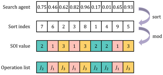
Figure 1. SOI-based encoding mapping.

Each solution vector $X^{\prime }$ corresponds to a processing order, which is a scheduling scheme. By this transformation, the feasibility of the scheduling scheme can be guaranteed without modifying the evolutionary operation of the algorithm. For example, in the scheduling sequence shown in Figure 1, there are three jobs, each containing three operations, and the number of occurrences of each job represents the corresponding operation from left to right. Since the processing machine and time for each operation are pre-specified (as shown in Table 3), the sequence of operations in Figure 1 can be decoded into the scheduling Gantt chart shown in Figure 2.

Table 3. A case of JSSP [36].

Jobs	(Mi, Ti)
	O1	O2	O3
1	(1, 10)	(3, 15)	(2, 5)
2	(2, 15)	(1, 8)	(3, 20)
3	(3, 9)	(2, 10)	(1, 15)

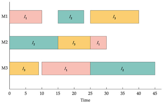
Figure 2. SOI-based decoding mapping.

3. Related Works

3.1. Slime Mould Algorithm

Slime Mould Algorithm (SMA) is a swarm-based metaheuristic algorithm developed by Li et al. in 2020 [22]. It simulates the behavioral and morphological changes of slime mould during foraging to find the best food source. The mathematical model for updating the location of slime mould is seen in Equation (3):

$$\overrightarrow{X(t+1)}=\{\begin{array}{ll}rand·(UB-LB)+LB\hfill & rand<z\hfill \\ \overrightarrow{X_b(t)}+\overrightarrow{vb}·(\overrightarrow{W}·\overrightarrow{X_A(t)}-\overrightarrow{X_B(t)})\hfill & r<p\hfill \\ \overrightarrow{vc}·\overrightarrow{X(t)}\hfill & r\ge p\hfill \end{array}$$

(3)

where $LB$ and $UB$ denote the lower and upper bounds of the search range, $rand$ and $r$ denote random numbers in [0, 1], $z=0.03$ is an adjustable parameter, $\overrightarrow{X_b(t)}$ is the best location found so far, $\overrightarrow{vb}$ and $\overrightarrow{vc}$ are random parameter vectors, $\overrightarrow{vb}$ takes values in $[-a,a]$, $\overrightarrow{vc}$ decreases linearly as the number of iterations $t$ goes from 1 to 0, $\overrightarrow{W}$ is the thickness of the vein-like vessels, $\overrightarrow{X_A(t)}$ and $\overrightarrow{X_B(t)}$ are two randomly selected individual locations in the population, and $\overrightarrow{X(t)}$ indicates the location of slime mould.

The value of $p$ is calculated as Equation (4):

$$p=\tanh |S(i)-DF|$$

(4)

where $i\in 1,2,\dots ,n$, $S(i)$ denotes the fitness $\overrightarrow{X}$, and $DF$ denotes the best fitness value obtained so far.

The value of $a$ in the range of $\overrightarrow{vb}$ is calculated as Equation (5):

$$a=\mathrm{arctanh}\left(1-t/\max \_t\right)$$

(5)

where $\max \_t$ is the maximum number of iterations.

The formula of $\overrightarrow{W}$ is calculated as Equation (6):

$$\overrightarrow{W(SmellIndex(i))}=\{\begin{array}{ll}1+r·\log \left(\frac{bF-S(i)}{bF-wF}+1\right)\hfill & condition\hfill \\ 1-r·\log \left(\frac{bF-S(i)}{bF-wF}+1\right)\hfill & others\hfill \end{array}$$

(6)

$$\overrightarrow{SmellIndex}=sort(\overrightarrow{S})$$

(7)

where $condition$ denotes the individuals whose fitness $S(i)$ ranks in the top half, $r$ denotes a random number in [0, 1], $bF$ denotes the best fitness of the current iteration, $wF$ denotes the worst fitness of the current iteration, and $\overrightarrow{SmellIndex}$ denotes the result of ranking the fitness $S(i)$ in ascending order (in the minimization problem). The pseudo-code of SMA is shown in Algorithm 1 [22].

Algorithm 1: Pseudo-code of SMA

1. Initialize the parameters $z,max\_t,N,Dim$; 2. Initialize the locations of slime mould $\overrightarrow{X_i}(i=1,2,\cdots ,N)$; 3. While ($t\le max\_t$) 4.    Check the boundary and calculate the fitness $\overrightarrow{S}$; 5.    Sort the fitness $\overrightarrow{S}$; 6.    Update $bF,wF,DF,\overrightarrow{X_b}$; 7.    Calculate the $\overrightarrow{W}$ by Equation (6); 8.    Update $p,\overrightarrow{vb},\overrightarrow{vc},A,B$; 9.       For each search agents 10.       Update locations by Equation (3); 11.      End For 12.   $t=t+1$; 13. End While 14. Return$DF,\overrightarrow{X_b}$;

3.2. Equilibrium Optimizer

Faramarzi et al. [10] proposed the Equilibrium Optimizer (EO) in 2020, a novel optimization algorithm inspired by physical phenomena of control volume mass balance models. The mass balance equation is usually described by a first-order ordinary differential equation, as shown in Equation (8), which embodies the physical processes of entrance, departure, and generation of mass inside the control volume.

$$V\frac{dC}{dt}=Q{C}_{eq}-QC+G$$

(8)

Here, $V$ denotes the control volume, $C$ denotes the concentration within the control volume, $Q$ denotes the volume flow rate into or out of the control volume, $C_{eq}$ denotes the concentration when equilibrium is achieved, and $G$ denotes the mass generation rate in the control volume.

Equation (9) can be obtained by solving the ordinary differential equation described by Equation (8):

$$C=C_{eq}+\left(C_0-C_{eq}\right)F+\frac{G}{\lambda V}\left(1-F\right)$$

(9)

where $C_0$ is the concentration of the control volume at the initial start time $t_0$, $\lambda$ is the flow rate, and $F$ is the exponential term coefficient, which can be calculated by Equation (10).

$$F=\exp \left[-\lambda \left(t_1-t_0\right)\right]$$

(10)

The EO is mainly based on Equation (9) iterative optimization search. For an optimization problem, the concentration represents the individual solution, $C$ represents the solution generated by the current iteration, $C_0$ represents the solution obtained in the previous iteration, and $C_{eq}$ represents the best solution found so far.

To meet the optimization needs of different problems, the specific operation procedure and parameters of EO are designed as follows.

(1) Initialization: the algorithm performs random initialization within the upper and lower bounds of each optimization variable, as Equation (11):

$$C_i^0=C_{\min }+ran{d}_i\left(C_{\max }-C_{\min }\right),i=1,2,\cdots ,N$$

(11)

where $C_{\min }$ and $C_{\max }$ are the lower and upper bound of the optimization variables, respectively, and $ran{d}_i$ represents the random number vector for individual $i$, each element in [0, 1];

(2) Equilibrium pool: In order to improve the exploration capability of the algorithm and avoid falling into local optimum, the equilibrium state (i.e., the optimal individual) in Equation (9) will be selected from the five candidate solutions of the equilibrium pool, which is shown in Equation (12):

$$\overrightarrow{C_{eq,pool}}=\left\{\overrightarrow{C_{eq,1}},\overrightarrow{C_{eq,2}},\overrightarrow{C_{eq,3}},\overrightarrow{C_{eq,4}},\overrightarrow{C_{eq,ave}}\right\}$$

(12)

where $\overrightarrow{C_{eq,1}},\overrightarrow{C_{eq,2}},\overrightarrow{C_{eq,3}},\overrightarrow{C_{eq,4}}$ are the four best solutions found so far, and $\overrightarrow{C_{eq,ave}}$ represents the average concentration of the four optimal solutions. The five solutions in the equilibrium pool are chosen as $\overrightarrow{C_{eq}}$ with equal probability;

(3) Exponential term factor $\overrightarrow{F}$: In order to better balance the exploration and exploitation capabilities of the algorithm, Equation (10) is improved as Equation (13).

$$\begin{array}{l}\overrightarrow{F}=a_1·sign\left(\overrightarrow{r}-0.5\right)·\left(e^{-\overrightarrow{\lambda }{t}_1}-1\right)\\ t_1={\left(1-t/\max \_t\right)}^{\left(a_{2}t/\max \_t\right)}\end{array}$$

(13)

where $a_1$ means the weight constant coefficient of the global search, the larger $a_1$ the stronger the exploration ability of the algorithm and the weaker the exploitation ability, $sign$ is the sign function, $\overrightarrow{r}$ and $\overrightarrow{\lambda }$ represent the random number vector, each element in [0, 1], $t$ is the number of current iterations, and $\max \_t$ is the maximum number of iterations;

(4) Mass generation rate $\overrightarrow{G}$: In order to enhance the exploitation capability of the algorithm, the generation rate is designed as Equation (14):

$$\begin{array}{l}\overrightarrow{G}=\overrightarrow{GCP}\left(\overrightarrow{C_{eq}}-\overrightarrow{\lambda }\overrightarrow{C}\right)\overrightarrow{F}\\ \overrightarrow{GCP}=\{\begin{array}{cc}0.5r_1& r_2\ge GP\\ 0& r_2<GP\end{array}\end{array}$$

(14)

where $\overrightarrow{GCP}$ is the vector of generation rate control parameter, $r_1$ and $r_2$ are random numbers in [0, 1], and $GP=0.5$ is the generation probability.

Finally, the individual solution can be updated as shown in Equation (15):

$$\overrightarrow{C}=\overrightarrow{C_{eq}}+(\overrightarrow{C}-\overrightarrow{C_{eq}})\overrightarrow{F}+\frac{\overrightarrow{G}}{\overrightarrow{\lambda }V}(1-\overrightarrow{F})$$

(15)

where $V=1$ is considered as a unit.

The pseudo-code of EO is shown in Algorithm 2 [10].

Algorithm 2: Pseudo-code of EO

1. Initialize the parameters $a_1,a_2,V,GP,\max \_t,N,Dim$; 2. Initialize the concentration in control volume $\overrightarrow{C_i}(i=1,2,\cdots ,N)$; 3. Initialize the equilibrium pool $\overrightarrow{C_{eq,pool}}$; 4. While ($t\le max\_t$) 5.    Check the boundary and calculate the fitness $FitC$; 6.    Update the equilibrium pool $\overrightarrow{C_{eq,pool}}$; 7.    Update $\overrightarrow{C}$ and $FitC$ with greedy strategy; 8.       For each search agents 9.         Update random variables $\overrightarrow{\lambda },\overrightarrow{r_n},r_1,r_2$; 10.       Randomly select the $\overrightarrow{C_{eq}}$ in the $\overrightarrow{C_{eq,pool}}$; 11.       Calculate the $\overrightarrow{F}$ and $\overrightarrow{G}$ by Equations (13) and (14); 12.       Update concentrations $\overrightarrow{C}$ by Equation (15); 13.      End For 14.   $t=t+1$; 15. End While 16. Return$\overrightarrow{C_{eq,1}}$ and its fitness;

3.3. Centroid Opposition-Based Computation

Centroid Opposition-based Computation (COBC) is an opposition-based computation scheme proposed by Rahnamayan et al. in 2014 [48]. Experimental results have shown that the average performance of COBC improves by 15% over conventional opposition-based computation method, which is a better improvement strategy. Interested readers can find a detailed description of COBC in [48]. The pseudo-code of COBC is shown in Algorithm 3.

Algorithm 3: Pseudo-code of COBC

1. Get initial location $\overrightarrow{X_i}(i=1,2,\cdots ,N)$; 2. Centroid point evaluation $\overrightarrow{M}=mean(\overrightarrow{X})$; 3. Centroid opposite population calculation $\overrightarrow{O{X}_i}=2\overrightarrow{M}-\overrightarrow{X_i}(i=1,2,\cdots ,N)$; 4. For each search agents 5.   Calculate the fitness of $\overrightarrow{OX}$; 6.      If $FitOX<FitX$ 7.      Update $\overrightarrow{X}$ and $FitX$ with greedy strategy; 8.      End If 9. End For 10. Return$\overrightarrow{X},FitX$;

3.4. Variable Neighborhood Search

Variable Neighborhood Search (VNS) [49] is a local search algorithm that uses alternating neighborhood structures composed of different actions to achieve a good balance between centralization and sparsity. The VNS is often used to solve combinatorial optimization problems, which rely on the fact: (1) the locally optimal solution of one neighborhood structure may not be the locally optimal solution of another neighborhood structure; (2) the globally optimal solution is the locally optimal solution of all possible neighborhoods. In order to enhance the local search capability of the metaheuristic algorithm for solving JSSP, a simplified VNS is introduced into the hybrid algorithm in this paper. The pseudo-code of the VNS is shown in Algorithm 4.

Algorithm 4: Pseudo-code of VNS

1. Get initialize solution $\overrightarrow{X}=\overrightarrow{X_0}$; 2. Calculate the fitness $FitX$ of $\overrightarrow{X}$; 3. Set $L=length(\overrightarrow{X})$; 4. While ($step\le L$) 5.    Take random integers $i$ and $j$ from 1 to $L$, and $i\ne j$; 6.    Update $\overrightarrow{XX}=Exchanging(\overrightarrow{X},i,j)$; 7.    Calculate the fitness $FitXX$ of $\overrightarrow{XX}$; 8.       If $FitXX<FitX$ 9.       Update $\overrightarrow{X}=\overrightarrow{XX}$ and $FitX=FitXX$; 10.      End If 11.   $step=step+1$; 12. End While 13. If$FitX<Fit{X}_0$ 14.      Return $\overrightarrow{X}$; 15. Else 16.      Return $\overrightarrow{X_0}$; 17. End If

The $Exchanging(\overrightarrow{X},i,j)$ executes a Two-point Exchange Neighborhood (TEN) [50], which implies exchanging the job operations in solution $\overrightarrow{X}$ between the ith and jth dimensions, its pseudo-code is shown in [32]. The example of the exchanging process is shown in Figure 3. It is worth noting that, unlike the setup in [32], in this paper, in order to reduce the time complexity of VNS, $Exchanging(\overrightarrow{X},i,j)$ does not evaluate all solutions of TEN (a total of $L\left(L-1\right)/2$ solutions); only $L$ solutions are randomly selected for evaluation and then the best solution among them is chosen.

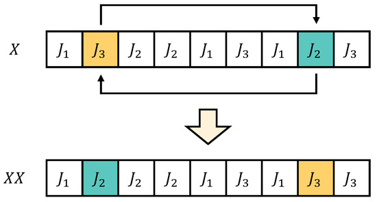
Figure 3. Exchanging process in VNS method [31].

4. Proposed EOSMA for JSSP

The shortcomings of the original SMA are unbalanced exploration and exploitation, weak exploration ability, and easy-to-fall-into local optimum. Changing the simple random search strategy in SMA to an equilibrium optimizer strategy can not only enhance the exploration ability but also improve the diversity of the population. The search agent of EOSMA performs a heuristic search based on the Equation (16):

$$\overrightarrow{X(t+1)}=\{\begin{array}{ll}\overrightarrow{X_{eq}(t)}+\left(\overrightarrow{X(t)}-\overrightarrow{X_{eq}(t)}\right)·\overrightarrow{F}+\overrightarrow{G}·\left(1-\overrightarrow{F}\right)/\overrightarrow{\lambda }V\hfill & rand<z\hfill \\ \overrightarrow{X_{eq,1}(t)}+\overrightarrow{vb}·\left(\overrightarrow{W}·\overrightarrow{X_A(t)}-\overrightarrow{X_B(t)}\right)\hfill & r<p\hfill \\ \overrightarrow{X(t)}+\overrightarrow{vc}·\overrightarrow{X(t)}\hfill & r\ge p\hfill \end{array}$$

(16)

where $z=0.6$ is an empirical value; $\overrightarrow{X_{eq}}$ denotes a randomly selected solution from the equilibrium pool; $\overrightarrow{X_{eq,1}}$ denotes the first solution in the equilibrium pool, i.e., the optimal solution found so far; and the remaining parameters in the Equation (16) use the settings of the original algorithm.

It is worth noting that all components of the solution vector of the first equation of Equation (16) are updated synchronously, independent of the next two equations, while the components of the solution vector of the second and third equations are updated separately; i.e., the same solution vector $\overrightarrow{X}$ may be updated using the second or third equation. Experiments show that asynchronous updates possess better performance than synchronous updates. In addition, EOSMA needs to update the equilibrium pool and the fitness weights of individuals at each generation, which increases the computational effort but does not increase the time complexity of the algorithm. Updating the equilibrium pool requires $O(n)$ and updating the fitness weights requires sorting the fitness and, therefore, requires $O(n\log n)$. Finally, EOSMA uses greedy selection repeatedly during iterations to speed up convergence, while SMA does not use the greedy strategy.

To further improve the performance of the hybrid algorithm for solving JSSP, the COBC strategy and the VNS strategy are introduced. The former enhances the exploration capability of the algorithm by selecting some individuals in each generation to perform the opposing computation; the latter is often used to solve combinatorial optimization problems, which is a local search algorithm framework that enhances the exploitation capability of the algorithm. The flow chart of EOSMA for solving JSSP is shown in Figure 4 and its pseudo-code is shown in Algorithm 5.

Algorithm 5: Pseudo-code of EOSMA for JSSP

1. Initialize the parameters $z,a_1,a_2,V,GP,max\_t,N,Dim,Jr$; 2. Initialize the locations of search agent $\overrightarrow{X_i}(i=1,2,\cdots ,N)$; 3. Calculate the fitness $FitX$ of $\overrightarrow{X}$; 4. Execute COBC to update the initial locations; 5. While ($t\le max\_t$) 6.    Calculate the fitness $FitX$; 7.       If ($rand<Jr$) 8.         Execute COBC to update individual locations; 9.       End If 10.   Retain better solutions compared to previous iteration; 11.   Sort the fitness $FitX$; 12.   Update the equilibrium pool $\overrightarrow{C_{eq,pool}}$; 13.   Update the $bF,wF$; 14.   Calculate the $\overrightarrow{W}$ by Equation (6); 15.      For each search agents 16.        Update locations $\overrightarrow{X}$ by Equation (16); 17.        Execute VNS to update individual locations; 18.      End For 19.   $t=t+1$; 20. End While 21. Return$\overrightarrow{X_{eq,1}}$ and its fitness;

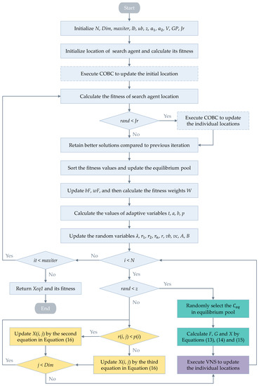
Figure 4. Flow chart of the EOSMA for JSSP.

5. Experimental Results and Discussions

In this paper, the performance of the EOSMA is evaluated by testing it on 82 test datasets taken from the OR Library. They are low-dimensional FT and ORB from [51,52], higher-dimensional LA and ABZ from [53,54], and high-dimensional YN and SWV from [55,56]. All experiments were executed on Win 10 Operating System and all algorithm codes were run in MATLAB R2019a with hardware details: Intel^® Core™ i7-9700 CPU (3.00 GHz) and 16 GB RAM.

For a fair comparison, the population size of all comparison algorithms was set to 25, the maximum number of iterations was set to 100, and all comparison algorithms were run 20 times independently on each dataset. In this paper, five algorithms were selected for comparison experiments with the EOSMA, namely SMA [22], EO [10], MPA [23], AO [20], and BES [21], which are the latest proposed algorithms with superior performance. For a fair comparison, all comparison algorithms incorporate the VNS strategy described in Algorithm 4. The specific parameters of the comparison algorithms are kept consistent with the original paper, as shown in Table 4. The performance of the algorithms is evaluated using the best fitness and the average fitness. The performance metrics are then ranked and the Friedman mean rank of the algorithms on different test instances is tallied; the experimental results are shown in Table 5, Table 6 and Table 7. In these tables, Instance denotes the case name; Size denotes the problem size, i.e., the number of jobs and machines; BKS denotes the best-known solution for that instance as reported by Liu et al. [36]; Best denotes the best fitness obtained by the algorithm; and Mean denotes the average fitness.

Table 4. Parameter settings of algorithms.

Algorithms	Parameter Settings
EOSMA	$z=0.6;a_1=2;a_2=1;V=1;GP=0.5;Jr=0.3$
VSMA	$z=0.03$
VEO	$a_1=2;a_2=1;V=1;GP=0.5$
VMPA	$FADs=0.2;P=0.5$
VAO	$\alpha =0.1;\delta =0.1$
VBES	$\alpha =2;a=10;R=1.5;c1=2;c2=2$

Table 5. Comparison of solution results of algorithms on FT and ORB.

Instances	Size	BKS	EOSMA		VSMA		VEO		VMPA		VAO		VBES
			Best	Mean	Best	Mean	Best	Mean	Best	Mean	Best	Mean	Best	Mean
FT06	6 × 6	55	55	55	55	58.05	55	55	55	55	55	56.65	55	55
FT10	10 × 10	930	942	978.95	954	1128.5	976	998.25	971	997.9	981	1033	983	1009.55
FT20	20 × 5	1165	1180	1212.45	1199	1335.15	1199	1234.45	1198	1240.2	1207	1245.4	1213	1254.45
Friedman mean rank			1.83	1.50	3.00	6.00	3.67	2.50	2.83	2.50	4.50	4.67	5.17	3.83
ORB01	10 × 10	1059	1086	1137.2	1090	1216.9	1104	1145.45	1122	1162	1104	1193.7	1141	1161.9
ORB02	10 × 10	888	899	926.5	902	986.85	921	936.65	894	945.3	931	965.6	920	940.35
ORB03	10 × 10	1005	1027	1089.2	1053	1223.7	1064	1109	1076	1108.25	1080	1166.8	1095	1126.8
ORB04	10 × 10	1005	1011	1043.4	1042	1195.25	1032	1059.7	1036	1064.65	1040	1084.65	1046	1063.55
ORB05	10 × 10	887	899	932.25	918	1019.35	909	952	899	951.95	920	996.15	910	961.1
ORB06	10 × 10	1010	1031	1060.45	1035	1154.45	1034	1082.75	1034	1090.9	1070	1156.7	1046	1098
ORB07	10 × 10	397	397	412.45	407	471.8	406	419.5	408	422.7	408	435.2	412	426.1
ORB08	10 × 10	899	916	966.15	942	1118.2	931	976.6	924	983.55	970	1037.35	934	986.9
ORB09	10 × 10	934	950	977.4	970	1097.15	969	984.5	962	993.75	957	1019.45	963	981.75
ORB10	10 × 10	944	957	983.3	983	1081.2	967	998.1	973	1003.5	1009	1047.8	955	1004.4
Friedman mean rank			1.25	1.00	4.00	5.90	3.20	2.30	3.05	3.20	4.90	5.10	4.60	3.50

The optimal values are shown in bold.

Table 6. Comparison of solution results of algorithms on ABZ and LA.

Instances	Size	BKS	EOSMA		VSMA		VEO		VMPA		VAO		VBES
			Best	Mean	Best	Mean	Best	Mean	Best	Mean	Best	Mean	Best	Mean
ABZ5	10 × 10	1234	1242	1259.55	1245	1340.5	1248	1271.5	1249	1266.45	1260	1297.5	1251	1272.15
ABZ6	10 × 10	943	947	964.75	948	1007.8	948	975.05	958	974.6	951	994.9	951	971.65
ABZ7	20 × 15	656	717	743.8	724	812.8	744	773.2	729	751.95	736	770.8	740	755.05
ABZ8	20 × 15	665	723	760.65	742	858.3	772	800.3	752	774	759	792.6	768	780.3
ABZ9	20 × 15	678	742	777.25	770	877.3	776	810.9	763	787.4	773	809.7	789	802.75
Friedman mean rank			1.00	1.00	2.30	6.00	4.50	4.40	3.60	2.20	4.50	4.40	4.50	3.00
LA01	10 × 5	666	666	666	666	692	666	666	666	666	666	670.7	666	666
LA02	10 × 5	655	655	665.3	655	718.05	655	669.2	655	674.55	655	690.35	655	666.7
LA03	10 × 5	597	597	612.55	611	667.5	606	619.5	605	624.35	617	640.75	604	617.75
LA04	10 × 5	590	590	598.15	590	638.75	590	601.8	590	604.25	599	618.45	590	601.8
LA05	10 × 5	593	593	593	593	596.8	593	593	593	593	593	593	593	593
LA06	15 × 5	926	926	926	926	948.35	926	926	926	926	926	926	926	926
LA07	15 × 5	890	890	890	890	958.4	890	890	890	891.65	890	894.35	890	890
LA08	15 × 5	863	863	863	863	894.9	863	863	863	863	863	866.45	863	863
LA09	15 × 5	951	951	951	951	979.65	951	951	951	951	951	951	951	951
LA10	15 × 5	958	958	958	958	973.2	958	958	958	958	958	958	958	958
LA11	20 × 5	1222	1222	1222	1222	1263.2	1222	1222	1222	1222	1222	1222	1222	1222
LA12	20 × 5	1039	1039	1039	1039	1081.15	1039	1039	1039	1039	1039	1039	1039	1039
LA13	20 × 5	1150	1150	1150	1150	1186.95	1150	1150	1150	1150	1150	1150	1150	1150
LA14	20 × 5	1292	1292	1292	1292	1302.15	1292	1292	1292	1292	1292	1292	1292	1292
LA15	20 × 5	1207	1207	1207	1207	1248.8	1207	1212.35	1207	1208.3	1207	1225.05	1207	1209.1
LA16	10 × 10	945	946	975.65	959	1090.25	946	982.2	959	990.75	988	1014.8	978	987.95
LA17	10 × 10	784	784	792.85	784	860.05	787	797.35	784	801	789	821.45	792	801.35
LA18	10 × 10	848	852	866.8	853	937.25	854	869	852	883.8	861	917.1	849	875.25
LA19	10 × 10	842	842	877.1	852	990.6	852	883.6	866	883.5	875	926.1	869	887.15
LA20	10 × 10	902	907	916.05	907	1005.45	907	928.65	907	929.05	924	961.85	914	934.2
LA21	15 × 10	1046	1081	1119.95	1117	1213.25	1111	1142.7	1089	1128.95	1105	1166.2	1104	1130.1
LA22	15 × 10	927	951	980.65	968	1071.75	964	1007.7	951	1011.15	997	1048.8	967	1008.4
LA23	15 × 10	1032	1032	1047	1032	1202.55	1042	1064.95	1032	1064.6	1037	1085.3	1032	1060.65
LA24	15 × 10	935	970	1008.95	984	1107.5	990	1029.5	987	1019.45	993	1042.25	994	1018.75
LA25	15 × 10	977	998	1046.5	1023	1114.85	1025	1070.9	1015	1060	1057	1111.7	1040	1066.35
LA26	20 × 10	1218	1225	1276.65	1251	1420.2	1290	1326.55	1256	1291.6	1273	1334.25	1249	1295.6
LA27	20 × 10	1235	1288	1346.4	1313	1513.95	1347	1380	1305	1358.05	1310	1383.95	1311	1361.3
LA28	20 × 10	1216	1256	1304.25	1279	1397.55	1311	1351.35	1284	1326.15	1285	1357.75	1285	1330.7
LA29	20 × 10	1152	1245	1288.3	1247	1411.7	1278	1338.85	1256	1310.55	1292	1345.3	1287	1315.4
LA30	20 × 10	1355	1355	1407.55	1387	1542.45	1399	1453.25	1407	1442.5	1407	1473.3	1396	1438.1
LA31	30 × 10	1784	1784	1785.4	1784	1947.6	1784	1818.05	1784	1794.2	1784	1800.4	1784	1786.1
LA32	30 × 10	1850	1850	1853.45	1850	1930.5	1863	1910.75	1850	1860.35	1850	1865.75	1850	1853.75
LA33	30 × 10	1719	1719	1722	1719	1879.6	1732	1774.9	1719	1725.65	1719	1748.8	1719	1722.65
LA34	30 × 10	1721	1721	1758.1	1750	1881.6	1790	1832.1	1722	1779.5	1747	1801.3	1743	1789.35
LA35	30 × 10	1888	1888	1895.85	1888	2043.65	1894	1935.9	1888	1909.65	1888	1935.6	1895	1932.75
LA36	15 × 15	1268	1311	1348.95	1336	1469.35	1359	1386.35	1334	1375.05	1362	1429.7	1350	1399.35
LA37	15 × 15	1397	1464	1524.65	1484	1717.7	1509	1559.45	1490	1535.55	1524	1602.1	1519	1565.15
LA38	15 × 15	1196	1280	1329.8	1281	1469.4	1309	1364.25	1300	1341.4	1334	1398.8	1335	1365.95
LA39	15 × 15	1233	1276	1337	1307	1479.8	1303	1366.3	1327	1376.4	1328	1424.25	1345	1377.5
LA40	15 × 15	1222	1269	1331.15	1277	1510.4	1300	1351.9	1312	1354	1327	1381	1316	1352.6
Friedman mean rank			2.23	1.50	3.24	6.00	4.01	3.26	3.11	2.85	4.51	4.48	3.90	2.91

The optimal values are shown in bold.

Table 7. Comparison of solution results of algorithms on YN and SWV.

Instances	Size	EOSMA		VSMA		VEO		VMPA		VAO		VBES
		Best	Mean	Best	Mean	Best	Mean	Best	Mean	Best	Mean	Best	Mean
YN1	20 × 20	985	1013.3	993	1121.85	1034	1064.95	990	1035.2	991	1047.4	1002	1038.25
YN2	20 × 20	1004	1052.25	1024	1148.2	1061	1095.5	1013	1055.1	1024	1070.65	1033	1067.6
YN3	20 × 20	982	1034.15	1017	1245.4	1045	1086.6	1018	1050.05	995	1062.3	1031	1061.05
YN4	20 × 20	1084	1124.3	1094	1268.5	1138	1179.95	1070	1142.1	1136	1180.5	1127	1156.85
Friedman mean rank		1.25	1.00	3.38	6.00	6.00	4.75	2.25	2.00	3.38	4.25	4.75	3.00
SWV01	20 × 10	1590	1684.55	1639	1747.85	1693	1754.85	1646	1728.8	1699	1791.9	1720	1765.75
SWV02	20 × 10	1653	1723.35	1652	1908.65	1730	1777.7	1709	1756.1	1716	1806.5	1745	1785.85
SWV03	20 × 10	1588	1650.7	1627	1790.35	1640	1727.25	1621	1688.45	1654	1754.85	1674	1712.9
SWV04	20 × 10	1655	1727.9	1713	1884.5	1735	1789.45	1705	1760.2	1661	1785.7	1733	1777.25
SWV05	20 × 10	1620	1706.2	1649	1941.2	1684	1743.6	1681	1722.15	1666	1747.1	1678	1718.05
SWV06	20 × 15	1964	2036.95	2009	2286.95	2045	2147.85	2001	2069.05	1957	2098.35	2044	2080.25
SWV07	20 × 15	1832	1935.95	1907	2148.9	1928	2022.1	1906	1960.65	1890	1985	1912	1962.15
SWV08	20 × 15	2024	2152.05	2120	2473.1	2182	2252.9	2076	2173.7	2129	2211.05	2122	2176.75
SWV09	20 × 15	1893	1981.4	1942	2288	1992	2101.9	1973	2034.9	1975	2066.7	2007	2047.45
SWV10	20 × 15	2007	2085	2071	2246.3	2132	2192.25	2001	2123.05	2033	2149.15	2073	2118.65
SWV11	50 × 10	3750	3877.35	3722	3951.2	3843	4063.8	3786	3913.25	3574	3739.1	3991	4042.8
SWV12	50 × 10	3755	3924.65	3845	4190.9	3906	4052.75	3851	3989.95	3702	3784.95	3955	4046.8
SWV13	50 × 10	3818	3933.3	3771	3991.25	4012	4128.65	3953	4041.35	3622	4041.5	4051	4137
SWV14	50 × 10	3690	3759.4	3676	3959.8	3815	3955.25	3774	3863.6	3514	3614.4	3825	3941.75
SWV15	50 × 10	3662	3829.55	3737	4008.25	3848	3991.75	3783	3879.65	3559	3669.45	3914	4020.75
SWV16	50 × 10	2924	2924	2924	3112.95	2924	2924.3	2924	2924	2924	2924	2924	2924
SWV17	50 × 10	2794	2794	2794	2932.5	2794	2810.25	2794	2794	2794	2799.15	2794	2796.1
SWV18	50 × 10	2852	2852	2852	3028.9	2852	2852.75	2852	2852	2852	2852.9	2852	2852
SWV19	50 × 10	2843	2847.3	2843	3014.5	2871	2955.2	2843	2853.75	2843	2878.55	2843	2864.25
SWV20	50 × 10	2823	2823	2823	3005.25	2823	2827	2823	2823.2	2823	2828.4	2823	2823
Friedman mean rank		2.15	1.38	2.90	5.50	4.95	4.65	3.25	2.40	2.80	3.68	4.95	3.40

The optimal values are shown in bold.

From Table 5, we can know that EOSMA can obtain better results on the low-dimensional JSSP. The results show that for the FT instance, EOSMA achieves the best results on all three instances and finds BKS on FT06. For the ORB instance, EOSMA achieves the best average performance on 10 instances; finds better solutions than other algorithms on 8 instances; and obtains BKS on ORB07, while VMPA and VBES, respectively, achieve the best results on ORB2 and ORB10 obtained the best solutions. Thus, EOSMA has good performance in solving JSSP-related problems compared to the recently proposed metaheuristic algorithms.

From Table 6, it can be seen that EOSMA can effectively solve JSSP. For 45 instances of LA and ABZ, EOSMA can obtain better performance metrics than other algorithms on all instances except LA18 where the best result is obtained by VBES and find BKS on 24 instances of LA. This shows that EOSMA overcomes the SMA exploration capability shortcomings, and its global search capability is stronger than the latest proposed algorithm to avoid falling into local optimum.

Table 7 presents the algorithm’s solution results on the high-dimensional JSSP; the optimal solution on these instances has not been found yet, so only approximate solutions obtained by different algorithms can be compared. The experimental results show that VAO shows a competitive advantage on high-dimensional instances, achieving better solutions than EOSMA on six instances of SWV, and VMPA achieves the best solutions on YN4 and SWV10, respectively; however, the average solution performance is inferior to that of EOSMA. Therefore, EOSMA still has better performance than other comparative algorithms on high-dimensional JSSP, verifying the effectiveness, accuracy, and robustness of EOSMA on the JSSP.

The execution times of the algorithms are shown in Figure 5 and Figure 6. Figure 5 represents the total time consumed by the six algorithms running 20 times on the six case datasets and Figure 6 shows the average single run times of the six algorithms on the 82 datasets.

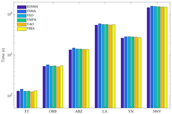
Figure 5. Execution time of six algorithms running 20 times.

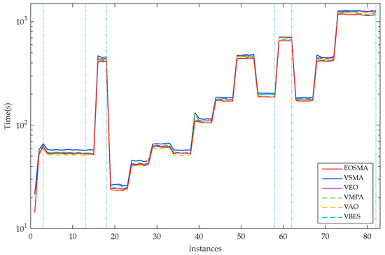
Figure 6. Average execution time of six algorithms on all instances.

As can be seen from Figure 5 and Figure 6, the execution time of EOSMA is the shortest among the six well-known comparison algorithms on ABZ, LA, YN, and SWV. The VAO has the shortest execution time on FT and ORB, followed by EOSMA, VEO, and VMPA. Since all six algorithms introduce the neighborhood search strategy, the main time consumption also comes from VNS but the execution time of EOSMA is significantly lower than VSMA on all instances. Particularly, the execution time of EOSMA is the shortest when solving the high-dimensional JSSP. It shows that EOSMA not only outperforms the well-known comparison algorithms in terms of convergence accuracy and robustness, but also has a shorter execution time.

In order to further analyze the convergence process of EOSMA and the comparison algorithm, two instances are selected from each instance set and their convergence curves and box plots are drawn in Figure 7 and Figure 8. It can be concluded that the convergence speed of EOSMA is faster than VSMA and VEO, and the final convergence accuracy is also better. It is worth noting that VSMA without hybridized EO operator has the slowest convergence speed, which is mainly due to the fact that SMA does not use a greedy selection strategy during the iterative process and the second equation of the Equation (3) uses the optimal solution of the current generation instead of the optimal solution found so far. Although EOSMA does not converge as fast as VAO and VBES in the early stages, the latter tends to fall into a local optimum later in the iteration, suggesting that EOSMA strikes a better balance between exploration and exploitation. The box plot likewise shows that EOSMA can find better solutions than other algorithms, with an average performance better than the comparison algorithms and far better than VSMA.

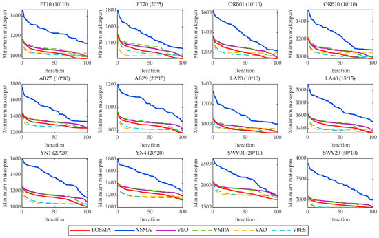
Figure 7. Average convergence curves of all comparison algorithms.

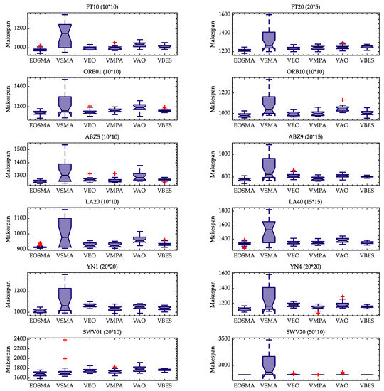
Figure 8. Box plots of all algorithms executed 20 times on instances.

The Wilcoxon rank-sum test [37] was performed to examine whether there was a statistically significant difference between the two sets of data, i.e., whether the results obtained by the algorithm were influenced by random factors. A similar comparison of statistical experiments is required to confirm the validity of the data because the metaheuristic algorithm is random [57]. The smaller the p-value, the greater the degree of confidence that there is a significant difference between the two data sets. When the p-value is less than 0.05, it indicates that the results obtained by the two algorithms are significantly different at the 95% confidence interval. Table 8 exhibits the results of the Wilcoxon p-value test for EOSMA and other well-known comparison algorithms.

Table 8. The p-value generated by Wilcoxon rank-sum test (two-tailed).

Instances	VSMA	VEO	VMPA	VAO	VBES	Instances	VSMA	VEO	VMPA	VAO	VBES
FT06	3.10 × 10−6	NaN	NaN	1.62 × 10−4	NaN	LA24	1.06 × 10−3	3.53 × 10−4	1.80 × 10−1	5.06 × 10−4	3.71 × 10−2
FT10	5.24 × 10−5	1.61 × 10−3	4.67 × 10−3	1.28 × 10−6	1.31 × 10−5	LA25	6.00 × 10−2	4.68 × 10−3	1.67 × 10−1	4.48 × 10−7	2.29 × 10−3
FT20	1.24 × 10−5	1.41 × 10−3	3.54 × 10−4	2.02 × 10−5	1.77 × 10−6	LA26	6.84 × 10−4	1.32 × 10−5	1.72 × 10−1	2.03 × 10−5	3.59 × 10−2
ORB01	1.02 × 10−2	4.49 × 10−1	1.78 × 10−3	6.23 × 10−6	8.31 × 10−4	LA27	2.34 × 10−3	1.78 × 10−4	2.79 × 10−1	1.28 × 10−3	2.94 × 10−2
ORB02	2.21 × 10−2	3.81 × 10−2	4.47 × 10−3	8.96 × 10−7	3.92 × 10−3	LA28	1.06 × 10−3	3.04 × 10−6	7.05 × 10−3	9.18 × 10−4	4.13 × 10−4
ORB03	9.62 × 10−4	6.98 × 10−2	2.47 × 10−2	3.26 × 10−6	2.87 × 10−4	LA29	2.15 × 10−2	8.54 × 10−6	3.37 × 10−2	7.07 × 10−6	9.62 × 10−4
ORB04	5.41 × 10−6	4.84 × 10−3	4.54 × 10−4	7.97 × 10−6	1.20 × 10−4	LA30	6.21 × 10−4	8.25 × 10−5	4.83 × 10−4	3.72 × 10−6	9.18 × 10−4
ORB05	1.43 × 10−4	3.25 × 10−2	2.56 × 10−2	5.86 × 10−6	2.21 × 10−4	LA31	3.76 × 10−5	1.19 × 10−7	1.07 × 10−2	2.03 × 10−4	3.50 × 10−1
ORB06	1.52 × 10−4	5.54 × 10−3	2.20 × 10−4	1.91 × 10−7	3.28 × 10−5	LA32	9.93 × 10−4	7.53 × 10−8	1.76 × 10−2	2.43 × 10−2	6.96 × 10−1
ORB07	6.93 × 10−5	1.70 × 10−2	1.40 × 10−3	2.72 × 10−5	8.46 × 10−6	LA33	7.85 × 10−6	3.88 × 10−8	4.03 × 10−1	2.87 × 10−4	1.62 × 10−1
ORB08	2.92 × 10−5	1.85 × 10−1	4.10 × 10−2	1.79 × 10−6	6.81 × 10−3	LA34	1.28 × 10−4	1.52 × 10−7	1.43 × 10−2	5.21 × 10−5	9.72 × 10−5
ORB09	3.27 × 10−5	5.46 × 10−2	1.65 × 10−2	6.20 × 10−5	3.16 × 10−1	LA35	2.08 × 10−2	5.62 × 10−7	7.78 × 10−2	1.69 × 10−4	7.96 × 10−7
ORB10	3.48 × 10−5	4.23 × 10−2	1.73 × 10−2	3.65 × 10−7	7.68 × 10−3	LA36	4.14 × 10−4	4.82 × 10−4	7.68 × 10−3	1.80 × 10−6	9.65 × 10−6
ABZ5	1.01 × 10−3	9.66 × 10−3	1.55 × 10−1	4.09 × 10−5	7.86 × 10−4	LA37	5.62 × 10−4	2.44 × 10−3	3.30 × 10−1	1.47 × 10−6	1.36 × 10−4
ABZ6	2.80 × 10−2	2.24 × 10−2	2.10 × 10−2	3.87 × 10−5	7.52 × 10−2	LA38	1.73 × 10−2	1.15 × 10−4	1.99 × 10−1	2.35 × 10−6	7.50 × 10−6
ABZ7	3.63 × 10−3	1.69 × 10−5	1.01 × 10−1	1.51 × 10−4	1.48 × 10−2	LA39	1.14 × 10−2	1.28 × 10−2	2.60 × 10−4	9.09 × 10−7	1.36 × 10−4
ABZ8	3.20 × 10−4	3.15 × 10−7	1.54 × 10−2	8.70 × 10−4	4.62 × 10−5	LA40	7.57 × 10−4	4.24 × 10−2	4.38 × 10−2	8.75 × 10−5	1.85 × 10−2
ABZ9	1.25 × 10−5	8.47 × 10−6	1.48 × 10−1	7.49 × 10−6	5.44 × 10−6	YN1	1.35 × 10−3	1.63 × 10−7	5.78 × 10−3	2.21 × 10−4	3.55 × 10−4
LA01	4.01 × 10−4	NaN	NaN	9.54 × 10−3	NaN	YN2	1.60 × 10−2	1.91 × 10−6	7.87 × 10−1	7.85 × 10−2	1.10 × 10−2
LA02	7.00 × 10−3	1.77 × 10−1	2.13 × 10−2	1.23 × 10−4	6.81 × 10−1	YN3	2.58 × 10−5	4.81 × 10−6	5.77 × 10−3	3.95 × 10−3	2.21 × 10−4
LA03	5.04 × 10−6	2.84 × 10−2	3.09 × 10−4	1.26 × 10−6	1.40 × 10−1	YN4	1.14 × 10−2	1.92 × 10−6	3.71 × 10−2	4.20 × 10−6	2.42 × 10−5
LA04	4.03 × 10−6	4.76 × 10−2	2.45 × 10−2	7.67 × 10−7	8.19 × 10−2	SWV01	2.73 × 10−1	1.04 × 10−4	8.68 × 10−3	5.81 × 10−6	2.84 × 10−6
LA05	4.53 × 10−3	NaN	NaN	NaN	NaN	SWV02	7.87 × 10−2	3.74 × 10−4	3.37 × 10−2	4.83 × 10−4	2.15 × 10−5
LA06	9.30 × 10−4	NaN	NaN	NaN	NaN	SWV03	1.18 × 10−2	2.44 × 10−5	2.00 × 10−2	1.67 × 10−6	5.99 × 10−7
LA07	1.10 × 10−6	NaN	8.06 × 10−2	9.58 × 10−3	NaN	SWV04	5.56 × 10−3	3.92 × 10−5	3.85 × 10−2	2.80 × 10−3	8.71 × 10−5
LA08	1.67 × 10−4	NaN	NaN	3.42 × 10−1	NaN	SWV05	3.96 × 10−3	1.67 × 10−2	3.72 × 10−1	1.61 × 10−2	3.58 × 10−1
LA09	6.68 × 10−5	NaN	NaN	NaN	NaN	SWV06	8.33 × 10−4	2.94 × 10−7	8.01 × 10−3	1.03 × 10−4	1.29 × 10−4
LA10	1.67 × 10−4	NaN	NaN	NaN	NaN	SWV07	5.34 × 10−4	3.05 × 10−6	2.08 × 10−1	3.48 × 10−2	9.07 × 10−2
LA11	1.67 × 10−4	NaN	NaN	NaN	NaN	SWV08	1.12 × 10−3	2.30 × 10−5	2.79 × 10−1	1.23 × 10−2	1.33 × 10−1
LA12	6.68 × 10−5	NaN	NaN	NaN	NaN	SWV09	1.16 × 10−4	6.65 × 10−6	1.95 × 10−3	4.66 × 10−5	1.89 × 10−4
LA13	2.57 × 10−5	NaN	NaN	NaN	NaN	SWV10	7.95 × 10−4	2.20 × 10−6	3.96 × 10−3	2.60 × 10−4	3.19 × 10−3
LA14	4.53 × 10−3	NaN	NaN	NaN	NaN	SWV11	4.82 × 10−1	3.98 × 10−6	3.98 × 10−2	6.86 × 10−4	6.77 × 10−8
LA15	9.58 × 10−3	9.58 × 10−3	1.63 × 10−1	6.67 × 10−5	8.06 × 10−2	SWV12	1.86 × 10−2	1.17 × 10−5	1.86 × 10−2	1.91 × 10−5	1.33 × 10−5
LA16	2.16 × 10−6	2.24 × 10−1	2.19 × 10−3	2.40 × 10−7	2.60 × 10−2	SWV13	1.26 × 10−1	2.56 × 10−7	3.48 × 10−5	1.89 × 10−4	1.65 × 10−7
LA17	1.07 × 10−5	1.57 × 10−2	7.11 × 10−3	5.16 × 10−6	7.84 × 10−4	SWV14	3.60 × 10−2	2.56 × 10−7	1.25 × 10−5	3.93 × 10−5	2.22 × 10−7
LA18	6.13 × 10−3	6.31 × 10−1	9.84 × 10−3	1.32 × 10−6	6.56 × 10−2	SWV15	6.79 × 10−2	8.06 × 10−6	2.15 × 10−2	1.17 × 10−5	1.57 × 10−6
LA19	1.89 × 10−5	1.43 × 10−1	9.66 × 10−2	8.85 × 10−7	1.31 × 10−2	SWV16	1.67 × 10−4	3.42 × 10−1	NaN	NaN	NaN
LA20	1.23 × 10−3	3.58 × 10−3	7.82 × 10−3	1.35 × 10−7	8.98 × 10−5	SWV17	4.53 × 10−3	1.67 × 10−4	NaN	8.06 × 10−2	8.06 × 10−2
LA21	1.10 × 10−5	5.30 × 10−4	1.04 × 10−1	1.36 × 10−4	1.13 × 10−1	SWV18	6.68 × 10−5	8.06 × 10−2	NaN	1.63 × 10−1	NaN
LA22	1.47 × 10−3	3.36 × 10−4	4.58 × 10−4	1.64 × 10−7	1.98 × 10−4	SWV19	1.62 × 10−5	3.46 × 10−8	4.38 × 10−2	1.75 × 10−3	3.65 × 10−4
LA23	7.89 × 10−4	5.90 × 10−4	1.99 × 10−2	9.08 × 10−6	9.34 × 10−3	SWV20	1.67 × 10−4	2.09 × 10−3	3.42 × 10−1	8.06 × 10−2	NaN

No significant differences are shown in bold.

The results of the Wilcoxon rank-sum test indicate that there are fewer instances without significant differences (as shown in bold), where NaN indicates that the two algorithms find exactly the same solution, in which case the optimal solution for that instance is usually found. Moreover, EOSMA significantly outperforms VSMA, VEO, VMPA, VAO, and VBES on 76, 60, 49, 69, and 53 instances, respectively, indicating that the algorithm has performance advantages on different instances of JSSP. In conclusion, the performance of EOSMA is significantly different from SMA, EO, and AO on JSSP; the results are statistically significant, indicating that the results obtained by EOSMA can be reproducibly achieved with more than 95% confidence.

6. Conclusions and Future Work

SMA is a novel swarm-based optimization algorithm inspired by the foraging behavior of slime mould; EO is a superior performance physics-based optimization algorithm inspired by the control volume mass balance equation. Although SMA has been applied in various fields due to the novelty of its metaheuristic rules, SMA still suffers from slow convergence, poor robustness, unbalanced exploration and exploitation, and the tendency to fall into local optimality. To overcome these drawbacks, we propose a hybrid algorithm, EOSMA, which uses a centroid opposition-based computation and VNS strategy combined with an SOI rule-based encoding method for fast and efficient solution of job shop scheduling problems. In EOSMA, the random search strategy of SMA is first replaced by the concentration update operator of EO and the third equation of Equation (3) is replaced by the third equation of Equation (16). Then, the centroid opposition-based calculation was introduced into the hybrid algorithm. With these changes, the search agent has a higher probability of finding a better solution and reduces the number of invalid searches, thus improving the exploration and exploitation capabilities of SMA. Finally, to solve JSSP more effectively, the two-point exchange neighborhood search strategy is added to EOSMA, which enhances the local search capability of EOSMA to solve JSSP. The performance of EOSMA was tested on 82 JSSP datasets from the OR Library and compared with recently proposed algorithms with superior performance. The experimental results show that EOSMA exhibits better search capability than SMA, EO, MPA, AO, and BES in solving JSSP.

JSSP is one of the well-known NP-hard problems. As the size increases, the search space of the problem increases dramatically and the execution time of many existing algorithms will increase dramatically, which cannot solve the larger scale job shop scheduling problem well. Additionally, EOSMA can effectively solve the larger scale JSSP in a reasonable running time. This is mainly because EOSMA not only relies on the local search capability of VNS but also has a strong global search capability before the local search, which can better guide the VNS strategy to find the optimal solution. Therefore, EOSMA is a promising algorithm. Future work will consider more practical scheduling problems, such as the flow shop scheduling problem considering material handling time and the permutation flow shop dynamic scheduling problem considering dynamic changes of processed raw materials, etc.

References

- Garey, M.R.; Johnson, D.S.; Sethi, R. The complexity of flowshop and jobshop scheduling. Math. Oper. Res. 1976, 1, 330–348. [Google Scholar] [CrossRef]
- Gong, G.; Deng, Q.; Chiong, R.; Gong, X.; Huang, H. An effective memetic algorithm for multi-objective job-shop scheduling. Knowl.-Based Syst. 2019, 182, 104840. [Google Scholar] [CrossRef]
- Tang, C.; Zhou, Y.; Tang, Z.; Luo, Q. Teaching-learning-based pathfinder algorithm for function and engineering optimization problems. Appl. Intell. 2021, 51, 5040–5066. [Google Scholar] [CrossRef]
- Grefenstette, J.J. Genetic algorithms and machine learning. Mach. Learn. 1988, 3, 95–99. [Google Scholar] [CrossRef]
- Storn, R.; Price, K. Differential evolution—A simple and efficient heuristic for global optimization over continuous spaces. J. Glob. Optim. 1997, 11, 341–359. [Google Scholar] [CrossRef]
- Kirkpatrick, S. Optimization by simulated annealing: Quantitative studies. J. Stat. Phys. 1984, 34, 975–986. [Google Scholar] [CrossRef]
- Rashedi, E.; Nezamabadi-pour, H.; Saryazdi, S. GSA: A gravitational search algorithm. Inf. Sci. 2009, 179, 2232–2248. [Google Scholar] [CrossRef]
- Mirjalili, S.; Mirjalili, S.M.; Hatamlou, A. Multi-verse optimizer: A nature-inspired algorithm for global optimization. Neural Comput. Appl. 2015, 27, 495–513. [Google Scholar] [CrossRef]
- Zhao, W.; Wang, L.; Zhang, Z. A novel atom search optimization for dispersion coefficient estimation in groundwater. Future Gener. Comput. Syst. 2018, 91, 601–610. [Google Scholar] [CrossRef]
- Faramarzi, A.; Heidarinejad, M.; Stephens, B.; Mirjalili, S. Equilibrium optimizer: A novel optimization algorithm. Knowl.-Based Syst. 2020, 191, 105190. [Google Scholar] [CrossRef]
- Eberhart, R.; Kennedy, J. A new optimizer using particle swarm theory. In Proceedings of the Sixth International Symposium on Micro Machine and Human Science, MHS’95, Nagoya, Japan, 4–6 October 1995; IEEE: Nagoya, Japan, 1995; pp. 39–43. [Google Scholar]
- Karaboga, D.; Basturk, B. A powerful and efficient algorithm for numerical function optimization: Artificial Bee Colony (ABC) algorithm. J. Glob. Optim. 2007, 39, 459–471. [Google Scholar] [CrossRef]
- Cuevas, E.; Cienfuegos, M.; Zaldívar, D.; Pérez-Cisneros, M. A swarm optimization algorithm inspired in the behavior of the social-spider. Expert Syst. Appl. 2013, 40, 6374–6384. [Google Scholar] [CrossRef]
- Mirjalili, S.; Mirjalili, S.M.; Lewis, A. Grey wolf optimizer. Adv. Eng. Softw. 2014, 69, 46–61. [Google Scholar] [CrossRef]
- Mirjalili, S.; Lewis, A. The whale optimization algorithm. Adv. Eng. Softw. 2016, 95, 51–67. [Google Scholar] [CrossRef]
- Dhiman, G.; Kumar, V. Seagull optimization algorithm: Theory and its applications for large-scale industrial engineering problems. Knowl.-Based Syst. 2018, 165, 169–196. [Google Scholar] [CrossRef]
- Mirjalili, S.; Gandomi, A.H.; Mirjalili, S.Z.; Saremi, S.; Faris, H.; Mirjalili, S.M. Salp swarm algorithm: A bio-inspired optimizer for engineering design problems. Adv. Eng. Softw. 2017, 114, 163–191. [Google Scholar] [CrossRef]
- Heidari, A.A.; Mirjalili, S.; Faris, H.; Aljarah, I.; Mafarja, M.; Chen, H. Harris hawks optimization: Algorithm and applications. Future Gener. Comput. Syst. 2019, 97, 849–872. [Google Scholar] [CrossRef]
- Rao, R.V.; Savsani, V.J.; Vakharia, D.P. Teaching–learning-based optimization: A novel method for constrained mechanical design optimization problems. Comput.-Aided Des. 2011, 43, 303–315. [Google Scholar] [CrossRef]
- Abualigah, L.; Yousri, D.; Abd Elaziz, M.; Ewees, A.A.; Al-qaness, M.A.A.; Gandomi, A.H. Aquila optimizer: A novel meta-heuristic optimization algorithm. Comput. Ind. Eng. 2021, 157, 107250. [Google Scholar] [CrossRef]
- Alsattar, H.A.; Zaidan, A.A.; Zaidan, B.B. Novel meta-heuristic bald eagle search optimisation algorithm. Artif. Intell. Rev. 2020, 53, 2237–2264. [Google Scholar] [CrossRef]
- Li, S.; Chen, H.; Wang, M.; Heidari, A.A.; Mirjalili, S. Slime mould algorithm: A new method for stochastic optimization. Future Gener. Comput. Syst. 2020, 111, 300–323. [Google Scholar] [CrossRef]
- Faramarzi, A.; Heidarinejad, M.; Mirjalili, S.; Gandomi, A.H. Marine predators algorithm: A nature-inspired metaheuristic. Expert Syst. Appl. 2020, 152, 113377. [Google Scholar] [CrossRef]
- Braik, M.S. Chameleon swarm algorithm: A bio-inspired optimizer for solving engineering design problems. Expert Syst. Appl. 2021, 174, 114685. [Google Scholar] [CrossRef]
- Bogar, E.; Beyhan, S. Adolescent Identity Search Algorithm (AISA): A novel metaheuristic approach for solving optimization problems. Appl. Soft Comput. 2020, 95, 106503. [Google Scholar] [CrossRef]
- Kurdi, M. An effective new island model genetic algorithm for job shop scheduling problem. Comput. Oper. Res. 2016, 67, 132–142. [Google Scholar] [CrossRef]
- Song, X.Y.; Meng, Q.H.; Yang, C. Improved taboo search algorithm for job shop scheduling problems. Syst. Eng. Electron. 2008, 30, 93–96. [Google Scholar] [CrossRef]
- Aydin, M.E.; Fogarty, T.C. A distributed evolutionary simulated annealing algorithm for combinatorial optimisation problems. J. Heuristics 2004, 10, 269–292. [Google Scholar] [CrossRef]
- Zhang, J.; Wang, W.; Xu, X. A hybrid discrete particle swarm optimization for dual-resource constrained job shop scheduling with resource flexibility. J. Intell. Manuf. 2017, 28, 1961–1972. [Google Scholar] [CrossRef]
- Huang, R.-H.; Yu, T.-H. An effective ant colony optimization algorithm for multi-objective job-shop scheduling with equal-size lot-splitting. Appl. Soft Comput. 2017, 57, 642–656. [Google Scholar] [CrossRef]
- Banharnsakun, A.; Sirinaovakul, B.; Achalakul, T. Job shop scheduling with the best-so-far ABC. Eng. Appl. Artif. Intell. 2012, 25, 583–593. [Google Scholar] [CrossRef]
- Keesari, H.S.; Rao, R.V. Optimization of job shop scheduling problems using teaching-learning-based optimization algorithm. OPSEARCH 2014, 51, 545–561. [Google Scholar] [CrossRef]
- Dao, T.-K.; Pan, T.-S.; Nguyen, T.-T.; Pan, J.-S. Parallel bat algorithm for optimizing makespan in job shop scheduling problems. J. Intell. Manuf. 2018, 29, 451–462. [Google Scholar] [CrossRef]
- Wang, X.; Duan, H. A hybrid biogeography-based optimization algorithm for job shop scheduling problem. Comput. Ind. Eng. 2014, 73, 96–114. [Google Scholar] [CrossRef]
- Zhao, F.; Liu, Y.; Zhang, Y.; Ma, W.; Zhang, C. A hybrid harmony search algorithm with efficient job sequence scheme and variable neighborhood search for the permutation flow shop scheduling problems. Eng. Appl. Artif. Intell. 2017, 65, 178–199. [Google Scholar] [CrossRef]
- Liu, M.; Yao, X.; Li, Y. Hybrid whale optimization algorithm enhanced with Lévy flight and differential evolution for job shop scheduling problems. Appl. Soft Comput. 2020, 87, 105954. [Google Scholar] [CrossRef]
- Liu, C. An improved Harris hawks optimizer for job-shop scheduling problem. J. Supercomput. 2021, 77, 14090–14129. [Google Scholar] [CrossRef]
- Wei, Y.; Zhou, Y.; Luo, Q.; Deng, W. Optimal reactive power dispatch using an improved slime mould algorithm. Energy Rep. 2021, 7, 8742–8759. [Google Scholar] [CrossRef]
- Abdel-Basset, M.; Chang, V.; Mohamed, R. HSMA_WOA: A hybrid novel slime mould algorithm with whale optimization algorithm for tackling the image segmentation problem of chest X-ray images. Appl. Soft Comput. 2020, 95, 106642. [Google Scholar] [CrossRef]
- Liu, Y.; Heidari, A.A.; Ye, X.; Liang, G.; Chen, H.; He, C. Boosting slime mould algorithm for parameter identification of photovoltaic models. Energy 2021, 234, 121164. [Google Scholar] [CrossRef]
- Yu, K.; Liu, L.; Chen, Z. An improved slime mould algorithm for demand estimation of urban water resources. Mathematics 2021, 9, 1316. [Google Scholar] [CrossRef]
- Hassan, M.H.; Kamel, S.; Abualigah, L.; Eid, A. Development and application of slime mould algorithm for optimal economic emission dispatch. Expert Syst. Appl. 2021, 182, 115205. [Google Scholar] [CrossRef]
- Zhao, S.; Wang, P.; Heidari, A.A.; Chen, H.; Turabieh, H.; Mafarja, M.; Li, C. Multilevel threshold image segmentation with diffusion association slime mould algorithm and Renyi’s entropy for chronic obstructive pulmonary disease. Comput. Biol. Med. 2021, 134, 104427. [Google Scholar] [CrossRef] [PubMed]
- Yu, C.; Asghar Heidari, A.; Xue, X.; Zhang, L.; Chen, H.; Chen, W. Boosting quantum rotation gate embedded slime mould algorithm. Expert Syst. Appl. 2021, 181, 115082. [Google Scholar] [CrossRef]
- Rizk-Allah, R.M.; Hassanien, A.E.; Song, D. Chaos-opposition-enhanced slime mould algorithm for minimizing the cost of energy for the wind turbines on high-altitude sites. ISA Trans. 2021, 121, 191–205. [Google Scholar] [CrossRef] [PubMed]
- Houssein, E.H.; Mahdy, M.A.; Blondin, M.J.; Shebl, D.; Mohamed, W.M. Hybrid slime mould algorithm with adaptive guided differential evolution algorithm for combinatorial and global optimization problems. Expert Syst. Appl. 2021, 174, 114689. [Google Scholar] [CrossRef]
- Premkumar, M.; Jangir, P.; Sowmya, R.; Alhelou, H.H.; Heidari, A.A.; Chen, H. MOSMA: Multi-objective slime mould algorithm based on elitist non-dominated sorting. IEEE Access 2021, 9, 3229–3248. [Google Scholar] [CrossRef]
- Rahnamayan, S.; Jesuthasan, J.; Bourennani, F.; Salehinejad, H.; Naterer, G.F. Computing opposition by involving entire population. In Proceedings of the 2014 IEEE Congress on Evolutionary Computation (CEC), Beijing, China, 6–11 July 2014; IEEE: Beijing, China, 2014; pp. 1800–1807. [Google Scholar]
- Hansen, P.; Mladenović, N.; Moreno Pérez, J.A. Variable neighbourhood search: Methods and applications. 4OR 2008, 6, 319–360. [Google Scholar] [CrossRef]
- Gao, L.; Li, X.; Wen, X.; Lu, C.; Wen, F. A hybrid algorithm based on a new neighborhood structure evaluation method for job shop scheduling problem. Comput. Ind. Eng. 2015, 88, 417–429. [Google Scholar] [CrossRef]
- Fisher, H.; Thompson, G.L. Probabilistic Learning Combinations of Local Job-Shop Scheduling Rules. Industrial Scheduling; Prentice-Hall: Hoboken, NJ, USA, 1963; pp. 225–251. [Google Scholar]
- Applegate, D.; Cook, W. A computational study of the job-shop scheduling instance. ORSA J. Comput. 1991, 3, 149–156. [Google Scholar] [CrossRef]
- Adams, J.; Balas, E.; Zawack, D. The shifting bottleneck procedure for job shop scheduling. Manag. Sci. 1988, 34, 391–401. [Google Scholar] [CrossRef]
- Lawrence, S. Resource Constrained Project Scheduling: An Experimental Investigation of Heuristic Scheduling Techniques (Supplement); Graduate School of Industrial Administration, Carnegie-Mellon University: Pittsburgh, PA, USA, 1984. [Google Scholar]
- Yamada, T.; Nakano, R. A genetic algorithm applicable to large-scale job-shop instances. Parallel Instance Solving Nat. 1992, 2, 281–290. [Google Scholar]
- Storer, R.H.; Wu, S.D.; Vaccari, R. New search spaces for sequencing problems with application to job shop scheduling. Manag. Sci. 1992, 38, 1495–1509. [Google Scholar] [CrossRef]
- Yin, S.; Luo, Q.; Du, Y.; Zhou, Y. DTSMA: Dominant swarm with adaptive t-distribution mutation-based slime mould algorithm. Math. Biosci. Eng. 2022, 19, 2240–2285. [Google Scholar] [CrossRef] [PubMed]
Publisher’s Note: MDPI stays neutral with regard to jurisdictional claims in published maps and institutional affiliations. |
© 2022 by the authors. Licensee MDPI, Basel, Switzerland. This article is an open access article distributed under the terms and conditions of the Creative Commons Attribution (CC BY) license (https://creativecommons.org/licenses/by/4.0/).