Characterization of the Mean First-Passage Time Function Subject to Advection in Annular-like Domains

Abstract

Cell migration in a biological medium towards a blood vessel is modeled, as a random process, sucessively inside an annulus (two-dimensional domain) and an annular cylinder (three-dimensional domain). The conditional probability function u for the cell moving inside such domains (tissue) fulfills by assumption a diffusion–advection equation that is subject to a Dirichlet boundary condition on the outer boundary and a Robin boundary condition on the inner boundary. The mean first-passage time (MFPT) function determined by u estimates the average time for the travelling cell to reach various interesting targets. The MFPT function fulfills a Poisson equation inside a domain with suitable boundary conditions, which give rise to various mathematical problems. The main novelty of this study is the characterization of such an MFPT function inside an annulus and an annular cylinder, which is subject to a Robin boundary condition on the inner boundary and a Dirichlet boundary condition on the outer one, and these are integral functions whose densities are the solution of an inhomogeneous system of linear integral equations.

1. Introduction

Cell migration is a key process in a variety of biological phenomena, from embryonic development to immune responses and even cancer metastasis, as well as an inherently complex process influenced by multiple factors, including cell type, environmental conditions, and interactions with other cells or extracellular matrix components. See [1,2,3,4,5,6]. These factors can create different modes of migration that can be understood using statistical physics frameworks, especially the idea of random walks. Random-walk models consider cells as random walkers whose displacement is governed by both diffusion and advection, and they have been effectively used to describe the statistical behavior of cell migration. Diffusion accounts for the random, undirected component of cell movement, thus originating from the intrinsic stochasticity of the intracellular machinery. Advection, on the other hand, describes directed cell migration, such as chemotaxis where cells move along a chemical concentration gradient. See [7]. As a result, understanding the dynamics of cell migration is a fundamental problem in biological physics.

The mean first-passage time (MFPT) in cell migration refers to the average time it takes for a cell to reach a specific target location or cross a defined boundary for the first time. See [8,9,10]. The MFPT, fulfilling a Poisson equation subject to mixed Dirichlet–Neumann boundary conditions in different confined domains, has been widely studied in the last decades from analytical and numerical points of view. See [11,12] and their references. For instance, the study of the upper and lower bounds of the MFPT of a cell escape through a boundary region, satisfying a diffusion equation under mixed Dirichlet–Neumann boundary conditions, has been undertaken in [13]. The study of the asymptotic behavior of the MFPT in annulus geometries with inner and outer regions has been carried out in [14]. The characterization of the MFPT function in three-dimensional simply and doubly connected domains subject to Dirichlet and Neumann boundary conditions has been achieved previously in [15] by means of a system of inhomogeneous linear integral equations.

In this work, we consider a tissue filling a nonsimply connected finite domain $\mathsf{\Omega }$ and bounded by a smooth closed boundary $\mathsf{\Gamma }$. Inside $\mathsf{\Omega }$, a cell migrates towards a certain part of $\mathsf{\Gamma }$ so as to intravasate it into a blood vessel located outside $\mathsf{\Omega }$, and it is enclosed by $\mathsf{\Omega }$. The cell is subject to both diffusive and drift motions, the latter of which are characterized by a suitable vector $\nu$ whose magnitude will be assumed to be small. Let x and y be two arbitrary points in $\mathsf{\Omega }$. The conditional probability density (or transition probability) of a cell to be at x at time $t\ge 0$, being originated at y at time $t=0$, is supposed to be the solution $u(t,x,y)$ of the diffusion–advection equation

$$\begin{array}{c}\hfill \left(\frac{\partial }{\partial t}-D({\mathsf{\Delta }}_x+\nu ·{\nabla }_x)\right)u(t,x,y)=0,\end{array}$$

(1)

where $D>0$ is the diffusion coefficient, which is subject to the following conditions:

(A1)

$u(0,x,y)=\delta (x-y)$ for any $x,y\in \mathsf{\Omega }$;

(A2)

${\displaystyle \underset{t\to +\infty }{lim}{\int }_{\mathsf{\Omega }}u(t,x,y)dx=0}$ for any $y\in \mathsf{\Omega }$.

Here, $\delta$ stands for the Dirac delta function. The diffusion–advection equation describes the spatiotemporal behavior of cells undergoing both diffusion (random motion) and advection (directed motion) due to external factors, such as chemotaxis (movement in response to chemical gradients) or mechanical forces within the domain $\mathsf{\Omega }$.

The MFPT function T, at $y\in \mathsf{\Omega }$, is defined as

$$\begin{array}{c}\hfill T\left(y\right)={\int }_{\mathsf{\Omega }}{\int }_0^{+\infty }u(t,x,y)dtdx,\end{array}$$

(2)

where u is the solution of (1), which is subject to conditions (A1) and (A2). The MFPT function quantifies the average time it takes for a migrating cell to reach the domain boundary, which provides a probabilistic measure of the expected time for a cell to achieve a particular outcome, which is essential for understanding cell behavior and navigation.

Moreover, consider that z is a point on the boundary $\mathsf{\Gamma }$, and let $n\left(z\right)$ be the inner normal-unit vector at z on $\mathsf{\Gamma }$, and let the product $n\left(z\right)·\nabla f\left(z\right)\equiv \frac{\partial f\left(z\right)}{\partial n\left(z\right)}$ be the inner first derivative of the function f at z on $\mathsf{\Gamma }$. Assume that there are two disjoint regions ${\mathsf{\Gamma }}_D$ and ${\mathsf{\Gamma }}_R$ on the boundary $\mathsf{\Gamma }$ so that $\mathsf{\Gamma }={\mathsf{\Gamma }}_D\cup {\mathsf{\Gamma }}_R$, and the following boundary conditions are satisfied:

(B1)

(Dirichlet) ${\displaystyle \underset{y\to z}{lim}f\left(y\right)=0}$, for any z in a region ${\mathsf{\Gamma }}_D\subset \mathsf{\Gamma }$,

(B2)

(Robin) ${\displaystyle a\underset{y\to z}{lim}\frac{\partial f\left(y\right)}{\partial n\left(y\right)}+b\underset{y\to z}{lim}f\left(y\right)+c=0}$ for any z in a region ${\mathsf{\Gamma }}_R\subset \mathsf{\Gamma }$, with $a\ne 0$, b, and c given as real constants.

The Dirichlet and Robin boundary conditions describe how cells interact with the boundaries of the domain. The Dirichlet boundary condition (B1) prevents cells from leaving or entering through such a boundary so that they are constrained to remain within the tissue $\mathsf{\Omega }$. The Robin boundary condition (B2) is expressed as a combination of both the Dirichlet and Neumann boundary conditions. The Dirichlet component of the Robin boundary condition prevents cells from leaving or entering the domain, while the Neumann component accounts for the flux of cells at the boundary and represents the rate at which cells are allowed to move across such a boundary.

Notice that, in the MFPT function, the T defined in (2) solves the so-called adjoint equation

$$\begin{array}{c}\hfill D(\mathsf{\Delta }+\nu ·\nabla )T\left(y\right)=-1\end{array}$$

(3)

in $\mathsf{\Omega }$, which is subject to the boundary conditions (B1) and (B2) and the finiteness condition $0\le T\left(y\right)<+\infty$ in $\mathsf{\Omega }$. This is a direct generalization of the result, without drift ($\left|\nu \right|=0$), as stated in [15] (Proposition 2.3). See also [16,17].

Our aim is to first characterize the MFPT function when the domain $\mathsf{\Omega }$ is an annulus and then when it is an annular cylinder, thereby assuming the Dirichlet boundary condition (B1) on the outer boundary and the Robin boundary condition (B2) on the inner one. Therefore, in the next section, the explicit characterization of the MFPT function is achieved, assuming drift motion, when the domain is an annulus limited by two closed and nonintersecting curves. This domain intends to model the orthogonal projection into a plane of the tissue and the blood vessel. Then, in Section 3, the three-dimensional domain considered is an annular cylinder filled by tissue, which surrounds the blood vessel, thereby assuming no drift motion, for simplicity and satisfying the Dirichlet boundary condition (B1) on the outer boundary surface and the Robin boundary condition (B2) on the inner one. The main novelty in this study is to consider a diffusion–advection equation that is subject to a Robin boundary condition on the inner boundary of an annulus and an annular cylinder. In the last sections, the conclusions are stated and discussed. Supplementary justifications and discussions are presented in Appendix A and Appendix B for the two-dimensional case and in Appendix C for the three-dimensional one.

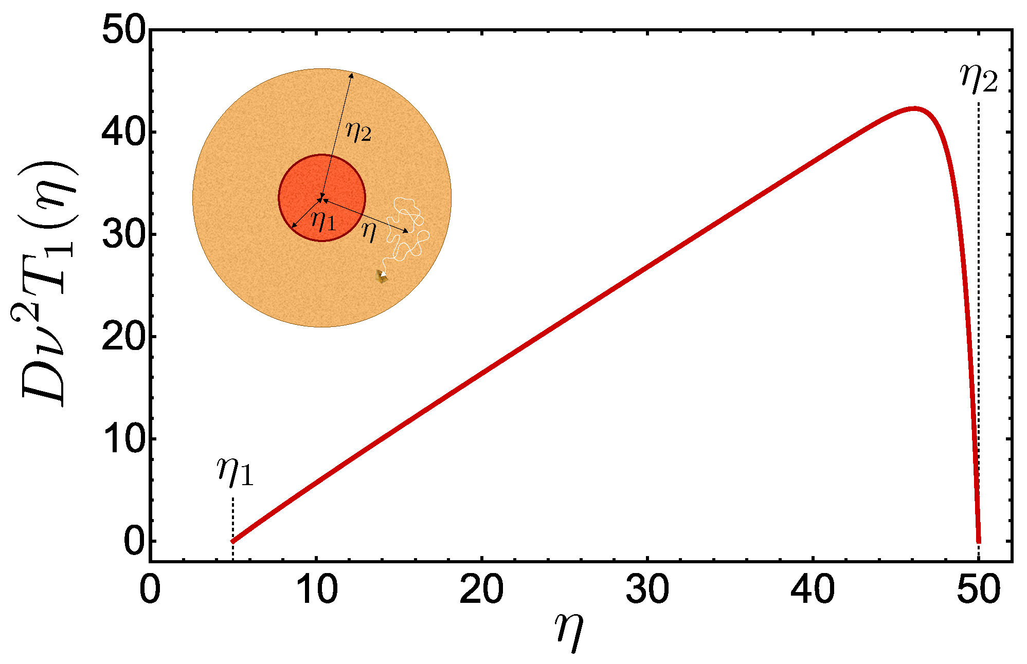
2. The MFPT Function in an Annulus

In this section, let us consider the following two dimensional domains:

• The domain ${\mathsf{\Omega }}_1$ is an annulus enclosed by two concentric circles ${\sigma }_1$ and ${\sigma }_2$, with radii $r_1$ and $r_2$, respectively ($r_1\le r_2$), so that the boundary is formed by the union of such circles;
• The domain ${\mathsf{\Omega }}_2$ is enclosed by two arbitrary smooth (differentiable) curves ${\sigma }_3$ and ${\sigma }_4$, which are obtained as small deformations of the previous concentric circles ${\sigma }_1$ and ${\sigma }_2$, respectively.

The first situation corresponds to a very idealized planar geometry for the tissue surrounding the blood vessel, while the second one tries to simulate a somewhat less-idealized planar geometry for the cross-section. Assume a radial drift on the cell directed towards the origin of coordinates, that is, $\nu =-\frac{\left|\nu \right|}{\rho }y$.

Proposition 1. 

Consider the domain ${\mathsf{\Omega }}_1$ with the Dirichlet boundary condition (B1) on the outer circle ${\sigma }_2$ and the Robin boundary condition (B2) on the inner circle ${\sigma }_1$. The MFPT function $T_1$ is given by

$$\begin{array}{c}\hfill T_1\left(\rho \right)=\left({\alpha }_2+\frac{1}{{D\left|\nu \right|}^2}\right){\int }_{\rho }^{r_2}\frac{e^{\left|\nu \right|\xi }}{\xi }d\xi -\frac{1}{{D\left|\nu \right|}^2}ln\left(\frac{r_2}{\rho }\right)-\frac{r_2-\rho }{D\left|\nu \right|},\end{array}$$

(4)

for every $\rho \in [r_1,r_2]$ for a suitable integration constant ${\alpha }_2$ so that ${\displaystyle a\underset{\rho \to r_1}{lim}\frac{d{T}_1\left(\rho \right)}{d\rho }+b\underset{\rho \to r_1}{lim}{T}_1\left(\rho \right)+c=0}$.

Proof. 

Upon taking the common center of ${\sigma }_1$ and ${\sigma }_2$ as the origin, the standard plane polar coordinates $\rho \ge 0$ and $\phi \in [0,2\pi )$ will be chosen so that $y=\rho (\cos \phi ,\sin \phi )$. Then, the adjoint Equation (3) may be written as

$$\begin{array}{c}\hfill \left(\frac{1}{\rho }\frac{\partial }{\partial \rho }\left(\rho \frac{\partial }{\partial \rho }\right)+\frac{1}{{\rho }^2}\frac{{\partial }^2}{\partial {\phi }^2}-\left|\nu \right|\frac{\partial }{\partial \rho }\right)T(\rho ,\phi )=-\frac{1}{D}.\end{array}$$

(5)

If the MFPT function has circular symmetry, that is, it is $\phi$-independent, then it may be defined as $T_1\left(\rho \right)$, thus being the solution of

$$\begin{array}{c}\hfill \left(\frac{1}{\rho }\frac{d}{d\rho }\left(\rho \frac{d}{d\rho }\right)-\left|\nu \right|\frac{d}{d\rho }\right)T_1\left(\rho \right)=-\frac{1}{D},\end{array}$$

(6)

which is a nonself-adjoint second-order linear differential equation. Without needing to transform it to a self-adjoint form, it can be solved directly so that

$$\begin{array}{c}\hfill T_1\left(\rho \right)={\alpha }_1+{\alpha }_2{\int }_{\rho }^{r_2}\frac{e^{\left|\nu \right|\xi }}{\xi }d\xi +\frac{1}{D}{\int }_{\rho }^{r_2}\frac{e^{\left|\nu \right|\xi }}{\xi }\left[\left(\frac{1-e^{-\left|\nu \right|\xi }}{\left|\nu \right|}\right)\xi +\frac{1}{\left|\nu \right|}\left(\frac{1-e^{-\left|\nu \right|\xi }}{\left|\nu \right|}-\xi \right)\right]d\xi ,\end{array}$$

where ${\alpha }_1$ and ${\alpha }_2$ are alternative pairs of arbitrary integration constants. Now, taking into account the boundary conditions, it follows that if the Dirichlet condition (B1) is assumed when $\rho =r_2$ on the circle ${\sigma }_2$, then $T_1\left(r_2\right)=0$. Particularly, ${\alpha }_1=0$. If the Robin boundary condition (B2) is imposed when $\rho =r_1$ on the circle ${\sigma }_1$, it follows that ${\displaystyle a\underset{\rho \to r_1}{lim}\frac{d{T}_1\left(\rho \right)}{d\rho }+b\underset{\rho \to r_1}{lim}{T}_1\left(\rho \right)+c=0}$, since $\frac{\partial }{\partial n\left(z\right)}=\frac{d}{d\rho }$, which gives an expression for ${\alpha }_2$. Simplifying it follows (4). □

As a particular case of the previous result, suppose two homogeneous Dirichlet boundary conditions that assume conditions (B1) and (B2), with $a=c=0$ and $b=1$, and make a change of the variable $\eta =\left|\nu \right|\rho$ with ${\eta }_1=\left|\nu \right|r_1$ and ${\eta }_2=\left|\nu \right|r_2$. The maximum of ${D\left|\nu \right|}^2{T}_1\left(\eta \right)$ is obtained at the root of the implicit equation:

$$\begin{array}{c}\hfill 1+\eta -\frac{({\eta }_2-{\eta }_1+\ln \left(\frac{{\eta }_2}{{\eta }_1}\right))e^{\eta }}{{\displaystyle {\int }_{\infty }^{{\eta }_2}\frac{e^t}{t}dt-{\int }_{\infty }^{{\eta }_1}\frac{e^t}{t}dt}}=0.\end{array}$$

When ${\eta }_1=\left|\nu \right|r_1=5$ and ${\eta }_2=\left|\nu \right|r_2=50$, Figure 1 displays the function ${D\left|\nu \right|}^2{T}_1\left(\eta \right)$.

Figure 1. The maximum MFPT is attained near the circle ${\sigma }_2$, thereby assuming Dirichlet boundary condition (B1) on both circles ${\sigma }_1$ and ${\sigma }_2$.

Now, as a less-idealized planar geometry for the projections of a tissue and the blood vessel onto an orthogonal plane to the latter, suppose that the arbitrary smooth curves ${\sigma }_3$ and ${\sigma }_4$ are approximately close to (or do not differ much from) two concentric circles ${\sigma }_1$ and ${\sigma }_2$, respectively. In other words, ${\sigma }_3$ and ${\sigma }_4$ are small or moderate deformations of ${\sigma }_1$ and ${\sigma }_2$, respectively. Consequently, the common center of the circles ${\sigma }_1$ and ${\sigma }_2$, even if not an exact center of symmetry for ${\sigma }_3$ and ${\sigma }_4$, does not differ much from a point playing such a role. Let ${\mathsf{\Omega }}_2$ be the domain enclosed by ${\sigma }_3$ and ${\sigma }_4$, and let that inside the annulus be ${\mathsf{\Omega }}_1$. The following representation of the MFPT function $T_2$ in (7) is given as the sum of a particular solution $T_1$ throughout all ${\mathsf{\Omega }}_1$, which is characterized in (4), plus as a general solution inside ${\mathsf{\Omega }}_2$ of the homogeneous equation $D\left(\mathsf{\Delta }+\nu ·\nabla \right)T\left(y\right)=0$, which is expressed as the sum of two closed-line integrals along ${\sigma }_3$ and ${\sigma }_4$ containing the densities ${\mu }_2$ and ${\mu }_1$, respectively.

Theorem 1. 

Consider the domain ${\mathsf{\Omega }}_2$, with the Dirichlet boundary condition (B1) on the outer curve ${\sigma }_4$ and the Robin boundary condition (B2) on the inner curve ${\sigma }_3$. The MFPT function $T_2$ is given by

$$\begin{array}{c}\hfill T_2\left(y\right)=T_1\left(\right|y\left|\right)+\frac{2D}{a}{\int }_{{\sigma }_3}G(y,\xi ){\mu }_1\left(\xi \right)d\sigma \left(\xi \right)-2D{\int }_{{\sigma }_4}\frac{\partial G(y,\xi )}{\partial n\left(\xi \right)}{\mu }_2\left(\xi \right)d\sigma \left(\xi \right),\end{array}$$

(7)

for every $y\in {\mathsf{\Omega }}_2$, where $T_1$ is defined in (4), G is the Green’s function, and the densities ${\mu }_1$ and ${\mu }_2$ are solutions of the system

$$\begin{array}{c}\hfill {\mu }_1\left(\xi \right)=\left(a\frac{\partial }{\partial n\left(\xi \right)}+b\right)\left(\frac{2D}{a}{\int }_{{\sigma }_3}G(\xi ,s){\mu }_1\left(s\right)d\sigma \left(s\right)-2D{\int }_{{\sigma }_4}\frac{\partial G(\xi ,s)}{\partial n\left(s\right)}{\mu }_2\left(s\right)d\sigma \left(s\right)\right)+\\ \hfill +\left(a\frac{\partial }{\partial n\left(\xi \right)}+b\right)T_1\left(\right|\xi \left|\right)+c,\end{array}$$

(8)

$$\begin{array}{c}{\mu }_2\left(\xi \right)=T_1\left(\right|\xi \left|\right)+\frac{2D}{a}{\int }_{{\sigma }_3}G(\xi ,s){\mu }_1\left(s\right)d\sigma \left(s\right)-2D{\int }_{{\sigma }_4}\frac{\partial G(\xi ,s)}{\partial n\left(s\right)}{\mu }_2\left(s\right)d\sigma \left(s\right).\end{array}$$

(9)

Proof. 

Let $G(y,y^{\prime })$ be the Green’s function, at $(y,y^{\prime })$ in the whole plane, so that

$$\begin{array}{c}\hfill D\left({\mathsf{\Delta }}_y+\nu ·{\nabla }_y\right)G(y,y^{\prime })=-\delta (y-y^{\prime }),\end{array}$$

(10)

where $\delta$ stands for the two-dimensional Dirac delta function, without any sort of Dirichlet or Robin boundary conditions either on ${\sigma }_2$ or ${\sigma }_1$, nor on ${\sigma }_4$ or ${\sigma }_3$. Notice that G includes angular dependences, which are certainly relevant for what follows. If $\left|\nu \right|=0$, then it follows that

$$\begin{array}{c}\hfill {\left.G(y,y^{\prime })\right|}_{\left|\nu \right|=0}=-\frac{1}{2\pi D}ln\left|y-y^{\prime }\right|,\end{array}$$

(11)

which has a logarithmic singularity as $\left|y-y^{\prime }\right|$ tends to 0.

The crucial features to obtain the density ${\mu }_2$ are explained below. Consider two close points $\xi$ and z lying on a small-line element ${\widehat{\sigma }}_4$ on the curve ${\sigma }_4$ and a point y lying inside ${\mathsf{\Omega }}_2$ and close to z so that the difference between $I{\left(y\right)}_{{\widehat{\sigma }}_4}$ and $I{\left(z\right)}_{{\widehat{\sigma }}_4}$ of the line integrals on ${\widehat{\sigma }}_4$ is

$$\begin{array}{c}\hfill I{\left(y\right)}_{{\widehat{\sigma }}_4}-I{\left(z\right)}_{{\widehat{\sigma }}_4}={\int }_{{\widehat{\sigma }}_4}\frac{\partial G(y,\xi )}{\partial n\left(\xi \right)}d\sigma \left(\xi \right)-{\int }_{{\widehat{\sigma }}_4}\frac{\partial G(z,\xi )}{\partial n\left(\xi \right)}d\sigma \left(\xi \right).\end{array}$$

(12)

According to Appendix A, the Green’s functions G (including drift) and ${\left.G\right|}_{\left|\nu \right|=0}$ (with vanishing drift) have the same short-distance behavior, since the operator $\nu ·\nabla$ is a weak perturbation of $\mathsf{\Delta }$. Then, it is permissible to replace G with ${\left.G\right|}_{\left|\nu \right|=0}$ in (12). The resulting integrals in (12) are extended to the complete closed curve ${\sigma }_4$. The added contributions to both integrals cancel out with each other. Thus, $I{\left(y\right)}_{{\widehat{\sigma }}_4}-I{\left(z\right)}_{{\widehat{\sigma }}_4}=I{\left(y\right)}_{{\sigma }_4}-I{\left(z\right)}_{{\sigma }_4}$, with

$$\begin{array}{c}\hfill I{\left(y\right)}_{{\sigma }_4}-I{\left(z\right)}_{{\sigma }_4}=-\frac{1}{2\pi D}\left({\int }_{{\sigma }_4}\frac{\partial \ln \left|y-\xi \right|}{\partial n\left(\xi \right)}d\sigma \left(\xi \right)-{\int }_{{\sigma }_4}\frac{\partial \ln \left|z-\xi \right|}{\partial n\left(\xi \right)}d\sigma \left(\xi \right)\right).\end{array}$$

Except for ${\left(2\pi D\right)}^{-1}$, these closed-line integrals are the full angles determined by the whole ${\sigma }_4$ as seen from two situations: either a point y lying strictly inside ${\mathsf{\Omega }}_2$, close to z, or inside z. By directly extending the argument in [18], those two dimensional angles are $2\pi$ and $\pi$, respectively. This statement will be illustrated through the following simple example. Let ${\sigma }_4$ be a circle of radius $r_4$, and let y be its center. Therefore, as $\frac{\partial }{\partial n\left(\xi \right)}$ denotes the inner normal derivative and $\left|\xi \right|=r_4$, it follows that ${\displaystyle 2\pi DI{\left(y\right)}_{{\sigma }_4}={\int }_{{\sigma }_4}\frac{1}{\left|\xi \right|}d\sigma \left(\xi \right)=2\pi }$. The actual counterpart of $I{\left(z\right)}_{{\sigma }_4}$, if the closed-line ${\sigma }_4$ is the boundary of a half circle and z is taken at the center, yields $\pi$. Thus, all that leads to the characterization of the density ${\mu }_2$ by (9). The extension of the above justification to the characterization of the density ${\mu }_1$ to the actual closed curve ${\sigma }_3$ in two dimensions with the drift and Robin boundary condition can also be carried out directly. For brevity, it will be omitted here. □

Models in two dimensions are plagued by a number of subtleties compared to models in three dimensions, as shown in the following very simplified model in Example 1, where the domain is only one circle. The structure of the integral equation approach in the proof of Theorem 1 is confirmed, and the important “averaging” recipe is introduced.

Example 1. 

Let Ω now be the interior of the full circle ${\sigma }_2$ of radius $r_2$, inside of which a cell moves randomly without drift, with the Dirichlet boundary condition. The circle ${\sigma }_1$ and, therefore, the Robin boundary condition are eliminated in this example. Accepting circular symmetry, the MFPT function $T_1$ solving Equation (6), with the Dirichlet boundary condition, is defined as follows:

$$\begin{array}{c}\hfill T_1\left(\rho \right)=\frac{r_2^2-{\rho }^2}{4D}.\end{array}$$

(13)

Consistency will be achieved if (13) is retrieved out of the following modified simplifications of (7) and (9). Namely, if the MFPT function $T_2$ is defined in (7), for any $y\in \mathsf{\Omega }$ and taking the density ${\mu }_2$ given in (9), then

$$\begin{array}{c}\hfill T_2\left(y\right)=T_1\left(\right|y\left|\right)-2D{\int }_{{\sigma }_2}\frac{\partial G(y,\xi )}{\partial n\left(\xi \right)}{\mu }_2\left(\xi \right)d\sigma \left(\xi \right)\end{array}$$

(14)

with

$$\begin{array}{c}\hfill {\mu }_2\left(\xi \right)=T_1\left(\right|\xi \left|\right)-2D{\int }_{{\sigma }_2}\frac{\partial G(\xi ,s)}{\partial n\left(s\right)}{\mu }_2\left(s\right)d\sigma \left(s\right),\end{array}$$

(15)

where $T_1\left(\right|y\left|\right)=-\frac{{\left|y\right|}^2}{4D}$, without drift. The density ${\mu }_2$ has supposed consistency, which depends only on $\rho =\left|\xi \right|$. By using (A1), (A5), and (15), noticing that the normal derivative is the inner one (towards the interior of the domain), and integrating over the angles (so that only $g_0(\rho ,{\rho }^{\prime })$ contributes), it follows that

$$\begin{array}{c}\hfill {\mu }_2\left(\xi \right)=T_1\left(\right|\xi \left|\right)-2D{r}_2{\mu }_2\left(r_2\right)\frac{\partial \ln {\rho }_{max}(\rho ,r_2)}{\partial {\rho }^{\prime }}\end{array}$$

(16)

where ${\rho }_{max}(\rho ,{\rho }^{\prime })=max\{\rho ,{\rho }^{\prime }\}$. When ${\rho }^{\prime }=r_2$, the derivative ${\displaystyle \frac{\partial \ln {\rho }_{max}(\rho ,r_2)}{\partial {\rho }^{\prime }}}$ is ambiguous so that some prescription will be required to handle it. By applying the “averaging” recipe in [15], we have

$${\displaystyle \frac{\partial \ln {\rho }_{max}(\rho ,r_2)}{\partial {\rho }^{\prime }}=\frac{1}{2}\left(\frac{\partial \ln {\rho }_{max}({\rho }^{+},{\rho }^{\prime })}{\partial {\rho }^{\prime }}+\frac{\partial \ln {\rho }_{max}({\rho }^{-},{\rho }^{\prime })}{\partial {\rho }^{\prime }}\right),}$$

where the first and second terms are evaluated for ${\rho }^{+}=\rho >{\rho }^{\prime }$ and ${\rho }^{\prime }>\rho ={\rho }^{-}$, respectively. The result is then $\frac{1}{2{\rho }^{\prime }}$, which becomes $\frac{1}{2r_2}$. In this way, the density ${\mu }_2$ in (16) is given by ${\mu }_2\left(\xi \right)=\frac{r_2^2}{4D}$. So, the second term on the right-hand side of (16) is of the same order as the left-hand side. The integral in (14) is directly computed for y inside Ω, which also uses $g_0(\rho ,{\rho }^{\prime })$ so that the above ambiguity does not arise. Therefore, $T_2\left(y\right)=T_1\left(\right|y\left|\right)+\frac{r_2^2}{4D}$, which consistently agrees with (13).

In Appendix B, an approximation method to characterize the densities ${\mu }_1$ and ${\mu }_2$ is presented whenever the curves ${\sigma }_3$ and ${\sigma }_4$ are close to the circles ${\sigma }_1$ and ${\sigma }_2$, respectively.

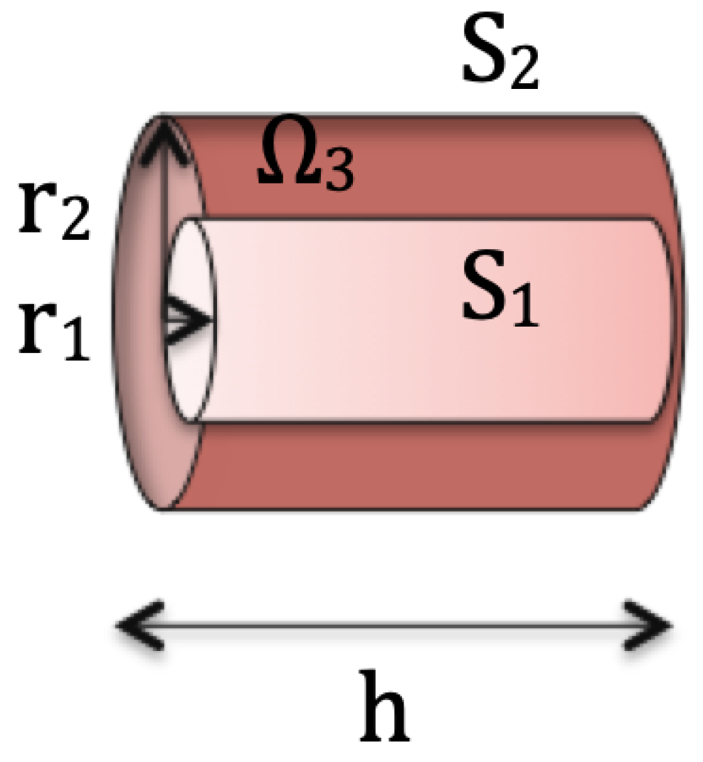
3. The MFPT Function in an Annular Cylinder

In this section, the three-dimensional domain is an annular cylinder filled by tissue, where a cell migrates inside it towards the blood vessel surrounded by it when there is no drift, that is, $\left|\nu \right|=0$ for simplicity. Namely, we consider the following cases:

• The domain ${\mathsf{\Omega }}_3$ is an annular cylinder limited by two parallel and concentric cylindrical surfaces $S_1$ and $S_2$, with radii $r_1$ and $r_2$, respectively, with $r_1<r_2$, and by two lids. Precisely, they are the finite intersections of two parallel planes (at a distance h from each other) with the cylinders and orthogonal to the axes of the latter; see Figure 2 below;
• By letting the two lids, in the previous case, be very separated from each other (as if h tends to infinity) so that they can be disregarded, the surface boundary will be supposed to be a small or moderate deformation of the two cylindrical surfaces in scenario 3.

Figure 2. The annular cylinder ${\mathsf{\Omega }}_3$ bounded by the inner surface $S_1$ and the outer surface $S_2$.

The domain ${\mathsf{\Omega }}_3$ corresponds to a very idealized cylindrical geometry for the tissue surrounding the blood vessel so that its analysis will rely on and constitute a nontrivial extension to three dimensions of the domain ${\mathsf{\Omega }}_1$, which was defined in the previous section.

Proposition 2. 

Consider the domain ${\mathsf{\Omega }}_3$, with the Dirichlet boundary condition (B1) on the outer surface $S_2$ and the Robin boundary condition (B2) on the inner surface $S_1$. The MFPT function $T_3$ is characterized in ${\mathsf{\Omega }}_3$, using cylindrical coordinates, by

$$\begin{array}{ccc}\hfill T_3(\rho ,z)& =& -\frac{2c_4}{h}{\int }_0^{+\infty }\sum _{k_z}\sin \left(k_z\frac{h}{2}\right)\frac{f_{k_{\rho }}\left(\rho \right)f_{k_z}\left(z\right)}{k_{\rho }^2+k_z^2}\frac{k_{\rho }}{k_z}\left[c_1(r_2{J}_1\left(k_{\rho }{r}_2\right)-r_1{J}_1\left(k_{\rho }{r}_1\right))+\right.\hfill \\ & & \left.+c_2(r_2{Y}_1\left(k_{\rho }{r}_2\right)-r_1{Y}_1\left(k_{\rho }{r}_1\right))\right]d{k}_{\rho },\hfill \end{array}$$

where $f_{k_{\rho }}\left(\rho \right)=c_1{J}_0\left(k_{\rho }\rho \right)+c_2{Y}_0\left(k_{\rho }\rho \right)$, $f_{k_z}\left(z\right)=c_3\sin \left(k_{z}z\right)+c_4\cos \left(k_{z}z\right)$, with $J_i$ and $Y_i$, for $i\in \{0,1\}$ being the standard regular and irregular Bessel functions of the ith order, respectively, for constants $c_1,c_2,$ and $c_4$, which are determined by the boundary conditions.

Proof. 

Let ${\sigma }_1$ and ${\sigma }_2$ be two concentric circles with radii $r_1$ and $r_2$, respectively, so that $r_1<r_2$, which are formed by the intersection of a plane with the two cylindrical surfaces $S_1$ and $S_2$ orthogonal to them, respectively. Upon taking the common center of ${\sigma }_1$ and ${\sigma }_2$ as the origin of the coordinates, the z axis through that point will be orthogonal to that plane. Consider the standard cylindrical coordinates $w=(\rho ,\phi ,z)$, with $y=(\rho \cos \phi ,\rho \sin \phi ,z)$, so that the three-dimensional domain ${\mathsf{\Omega }}_3$ may be defined as $r_1<\rho <r_2$, $0\le \phi <2\pi$, and $-\frac{h}{2}<z<\frac{h}{2}$. Then, the Laplacian operator in (3) may be written as

$$\begin{array}{c}\hfill \mathsf{\Delta }=\frac{1}{\rho }\frac{\partial }{\partial \rho }\left(\rho \frac{\partial }{\partial \rho }\right)+\frac{1}{{\rho }^2}\frac{{\partial }^2}{\partial {\phi }^2}+\frac{{\partial }^2}{\partial z^2}.\end{array}$$

Thus, take into account a MFPT function $T_3(\rho ,z)$ with circular symmetry ($\phi$-independent) solution of

$$\begin{array}{c}\hfill \left(\frac{1}{\rho }\frac{\partial }{\partial \rho }\left(\rho \frac{\partial }{\partial \rho }\right)+\frac{{\partial }^2}{\partial z^2}\right)T_3(\rho ,z)=-\frac{1}{D}\end{array}$$

(17)

in ${\mathsf{\Omega }}_3$. In addition, consider the Dirichlet boundary condition (B1), when $\rho =r_2$, so that $T_3(r_2,z)=0$, and consider the Robin boundary condition (B2), for $\rho =r_1$, so that ${\displaystyle a\underset{\rho \to r_1}{lim}\frac{\partial T_3(\rho ,z)}{\partial \rho }+b\underset{\rho \to r_1}{lim}{T}_3(\rho ,z)+c=0}$ for some constants a, b, and c. On the lids, when $z=-\frac{h}{2}$ and $z=\frac{h}{2}$, assume a homogeneous Robin boundary condition so that ${\displaystyle a\underset{\rho \to r_1}{lim}\frac{\partial T_3(\rho ,\pm \frac{h}{2})}{\partial \rho }+b\underset{\rho \to r_1}{lim}{T}_3\left(\rho ,\pm \frac{h}{2}\right)=0}$. For simplicity, the constants a and b are taken to be the same for the Robin boundary conditions at $\rho =r_1$ and at the two lids. The generalization for the different constants is direct and will be omitted.

The procedure to find out the MFPT function $T_3$ proceeds by applying well-documented procedures based upon suitable three-dimensional Green’s functions and representations thereof using separability, factorization, and eigenfunctions; see [19]. Thus, let $G_3(w,w^{\prime })$ be the Green’s function, in cylindrical coordinates, solution of the equation

$$\begin{array}{c}\hfill D\left(\frac{1}{\rho }\frac{\partial }{\partial \rho }\left(\rho \frac{\partial }{\partial \rho }\right)+\frac{{\partial }^2}{\partial z^2}\right)G_3(w,w^{\prime })=-\frac{1}{\rho }\delta (\rho -{\rho }^{\prime })\delta (z-z^{\prime }),\end{array}$$

so that

$$\begin{array}{c}\hfill G_3(w,w^{\prime })=\int \sum _{k_z}\frac{f_{k_{\rho }}\left(\rho \right)f_{k_z}\left(z\right)f_{k_{\rho }}\left({\rho }^{\prime }\right)f_{k_z}\left(z^{\prime }\right)}{k_{\rho }^2+k_z^2}d{k}_{\rho },\end{array}$$

with

$$\begin{array}{ccc}\hfill \int \sum _{k_z}{f}_{k_{\rho }}\left(\rho \right)f_{k_z}\left(z\right)f_{k_{\rho }}\left({\rho }^{\prime }\right)f_{k_z}\left(z^{\prime }\right)d{k}_{\rho }& =& \frac{1}{\rho }\delta (\rho -{\rho }^{\prime })\delta (z-z^{\prime })\hfill \end{array}$$

(18)

$$\begin{array}{ccc}\hfill D\left(\frac{1}{\rho }\frac{d}{d\rho }\left(\rho \frac{d}{d\rho }\right)\right)f_{k_{\rho }}\left(\rho \right)& =& -k_{\rho }^2{f}_{k_{\rho }}\left(\rho \right)\hfill \end{array}$$

(19)

$$\begin{array}{ccc}\hfill D\frac{d^2{f}_{k_z}\left(z\right)}{d{z}^2}& =& -k_z^2{f}_{k_z}\left(z\right).\hfill \end{array}$$

(20)

The solutions of Equations (19) and (20) may be written as $f_{k_{\rho }}\left(\rho \right)=c_1{J}_0\left(k_{\rho }\rho \right)+c_2{Y}_0\left(k_{\rho }\rho \right)$, where $J_0$ and $Y_0$ are the standard regular and irregular Bessel functions, respectively, of the zeroth order, and $f_{k_z}\left(z\right)=c_3\sin \left(k_{z}z\right)+c_4\cos \left(k_{z}z\right)$ for constants $c_1,c_2,c_3,$ and $c_4$, which are determined by imposing the boundary conditions. The boundary conditions for $f_{k_{\rho }}\left(\rho \right)$ at $r_1$ (inhomogeneous Robin condition) and $r_2$ (Dirichlet condition) are similar to those in the two-dimensional case for $\left|\nu \right|\ne 0$, and they will not be repeated again. In the case of the Robin boundary condition, if $c\ne 0$, then $k_{\rho }$ (real) varies continuously, and the constants $c_1$ and $c_2$ are uniquely defined by the inhomogeneous system. On the other hand, the homogeneous Robin boundary conditions for $f_{k_z}\left(z\right)$ at $z=\pm \frac{h}{2}$ make Equation (20) yield an eigenvalue equation for $k_z$, which has to take on a denumerably infinite set of values with the alternative choices: either $c_3=0$ and $c_4\ne 0$ for the eigenvalue equation $tan\left(k_z\frac{h}{2}\right)=-\frac{b}{a{k}_z}$ or $c_3\ne 0$ and $c_4=0$ for the eigenvalue equation $tan\left(k_z\frac{h}{2}\right)=\frac{a{k}_z}{b}$. The nonvanishing proportionality constant is determined through the completeness of Equation (18). Now, if the integration over ${\rho }^{\prime }$ and $z^{\prime }$ is performed, it follows, for $c_3=0$, that

$$\begin{array}{ccc}\hfill T_3(\rho ,z)& =& -{\int }_{r_1}^{r_2}{\int }_{-\frac{z_0}{2}}^{\frac{z_0}{2}}{\rho }^{\prime }{G}_3(w,w^{\prime })d{z}^{\prime }d{\rho }^{\prime }=\hfill \\ & =& -{\int }_0^{+\infty }\sum _{k_z}{c}_4\frac{f_{k_{\rho }}\left(\rho \right)f_{k_z}\left(z\right)}{k_{\rho }^2+k_z^2}\frac{\sin \left(k_z\frac{h}{2}\right)}{k_z\frac{h}{2}}\left(c_1{k}_{\rho }(r_2{J}_1\left(k_{\rho }{r}_2\right)-\right.\hfill \\ & & \left.r_1{J}_1\left(k_{\rho }{r}_1\right))+c_2{k}_{\rho }(r_2{Y}_1\left(k_{\rho }{r}_2\right)-r_1{Y}_1\left(k_{\rho }{r}_1\right))\right)d{k}_{\rho },\hfill \end{array}$$

where $J_1$ and $Y_1$ are the standard regular and irregular Bessel functions of the first order, respectively. In this way, the MFPT function is characterized in terms of an integral and a series. If $\frac{h}{2}$ tends to $+\infty$, the description in the two-dimensional case for $\left|\nu \right|=0$ is retrieved. □

Now, let us consider the domain ${\mathsf{\Omega }}_4$, where the geometry of the domain ${\mathsf{\Omega }}_3$ is considered and the two lids are suppressed so that the two cylindrical surfaces $S_1$ and $S_2$ extend along $-\infty <z<+\infty$. The boundary surface of the three-dimensional domain ${\mathsf{\Omega }}_4$ is formed by two surfaces, which are denoted by $S_3$ and $S_4$ and are very lengthy and moderate deformations of the above $S_1$ and $S_2$, respectively. Upon recalling that ${\mathsf{\Omega }}_3$ encloses ${\mathsf{\Omega }}_4$, the MFPT function $T_4$ defined below in (21) is the sum of a particular solution $T_1$ defined in (4) throughout all ${\mathsf{\Omega }}_3$, plus it is a solution of $D\mathsf{\Delta }T\left(y\right)=0$ inside ${\mathsf{\Omega }}_4$, which is expressed as the sum of two surface integrals along $S_3$ and $S_4$ containing ${\mu }_3$ and ${\mu }_4$, respectively. Notice that the MFPT function $T_4$ and the densities ${\mu }_3$ and ${\mu }_4$ are, in particular, z-dependent. When $S_i=S_{i-2}$, for $i\in \{3,4\}$, then ${\mu }_3=0$ and ${\mu }_4=0$, trivially.

Theorem 2. 

Consider the domain ${\mathsf{\Omega }}_4$ with the Dirichlet boundary condition (B1) on the outer surface $S_4$ and the Robin boundary condition (B2) on the inner surface $S_3$. The MFPT function $T_4$ is characterized in ${\mathsf{\Omega }}_4$ by

$$\begin{array}{c}\hfill T_4\left(y\right)=T_1\left(\right|y\left|\right)+\frac{2D}{a}{\int }_{S_3}{G}_3(y,x){\mu }_3\left(x\right)dS\left(x\right)-2D{\int }_{S_4}\frac{\partial G_3(y,x)}{\partial n\left(x\right)}{\mu }_4\left(x\right)dS\left(x\right),\end{array}$$

(21)

where the densities ${\mu }_3$ and ${\mu }_4$ are defined as solutions of the inhomogeneous system of linear integral equations:

$$\begin{array}{c}\hfill {\mu }_3\left(x\right)=\left(a\frac{\partial }{\partial n\left(x\right)}+b\right)\left(\frac{2D}{a}{\int }_{S_3}{G}_3(x,\xi ){\mu }_3\left(\xi \right)dS\left(\xi \right)-2D{\int }_{S_4}\frac{\partial G_3(x,\xi )}{\partial n\left(\xi \right)}{\mu }_4\left(\xi \right)dS\left(\xi \right)\right)\\ \hfill +\left(a\frac{\partial }{\partial n\left(x\right)}+b\right)T_1\left(\right|x\left|\right)+c,\end{array}$$

(22)

$$\begin{array}{c}\hfill {\mu }_4\left(x\right)=T_1\left(\right|x\left|\right)+\frac{2D}{a}{\int }_{S_3}{G}_3(x,\xi ){\mu }_3\left(\xi \right)dS\left(\xi \right)-2D{\int }_{S_4}\frac{\partial G_3(x,\xi )}{\partial n\left(\xi \right)}{\mu }_4\left(\xi \right)dS\left(\xi \right).\end{array}$$

(23)

Proof. 

For $i\in \{3,4\}$, each point $y_i$ on the surface $S_i$ may be written, in cylindrical coordinates, as $y_i=((r_i+{\epsilon }_i)\cos \phi ,(r_i+{\epsilon }_i)\sin \phi ,z+{\epsilon }_{z,i})$, where ${\epsilon }_i={\epsilon }_i\left(\phi \right)$ and ${\epsilon }_{z,i}={\epsilon }_{z,i}\left(z\right)$, with ${\epsilon }_{z,i}\left(z\right)$ tending to 0 as z tends to $\pm \infty$. This will enable the dependence of the MFPT function on z in ($-\infty ,+\infty$), in addition to those on $\phi$ and $\rho$, which will disappear quickly as z tends to $\pm \infty$. A very important assumption is that ${\mathsf{\Omega }}_4$, having $S_3$ and $S_4$ as boundaries, is contained inside the domain ${\mathsf{\Omega }}_3$ enclosed between $S_1$ and $S_2$. Let ${\sigma }_3$ and ${\sigma }_4$ be the two closed curves obtained as the intersections of the $z=0$ plane with the surfaces $S_3$ and $S_4$, respectively, so that they turn out to be small deformations of two concentric circles ${\sigma }_1$ and ${\sigma }_2$, respectively. The common center of such circles ${\sigma }_1$ and ${\sigma }_2$ plays the role of an approximate center of symmetry for ${\sigma }_3$ and ${\sigma }_4$.

Let $T_1\left(\right|y\left|\right)$ be the circularly symmetric MFPT function defined in (4) for any y in ${\mathsf{\Omega }}_1$, with the Dirichlet and Robin boundary conditions on ${\sigma }_2$ and ${\sigma }_1$, respectively. Let ${\displaystyle G_3(y,y^{\prime })=\frac{1}{4\pi D|y-y^{\prime }|}}$ be the standard three-dimensional Green’s function solution of $D{\mathsf{\Delta }}_y{G}_3(y,y^{\prime })=-\delta (y-y^{\prime })$ in the whole space, without any sort of Dirichlet or Robin boundary conditions. The expansion of $G_3$ in cylindrical coordinates $w=(\rho ,\phi ,z)$ is given by

$$\begin{array}{c}\hfill G_3(w,w^{\prime })=\frac{1}{4\pi D}\sum _{n=-\infty }^{+\infty }{e}^{in(\phi -{\phi }^{\prime })}{\int }_0^{+\infty }{e}^{-\kappa |z-z^{\prime }|}{J}_n\left(\kappa \rho \right)J_n\left(\kappa {\rho }^{\prime }\right)d\kappa ,\end{array}$$

(24)

where $J_n$ defines the standard regular Bessel functions of the nth order; see [19]. Let ${\displaystyle {\int }_{S_i}dS\left(x\right)}$ denote integration over the surface $S_i$ for $i\in \{3,4\}$. By extending the treatment of scenario 2 to the actual three-dimensional situation, it follows that the MFPT function $T_4\left(y\right)$ satisfying (3) for y inside ${\mathsf{\Omega }}_4$, with the Dirichlet and Robin boundary conditions on $S_4$ and $S_3$, respectively, is defined by (21), where the densities ${\mu }_3$ and ${\mu }_4$ are defined in $S_3$ and $S_4$, respectively, by the inhomogeneous system of linear integral Equations (22) and (23), respectively. □

Further information regarding the understanding of the densities ${\mu }_3$ and ${\mu }_4$ defined in (22) and (23), respectively, is given in Appendix C.

4. Discussion

The time-honored problem of adequately analyzing elliptic partial differential equations (in particular, in two and three spatial dimensions) inside a domain with a general boundary and prescribed boundary conditions continues to stand as an important and difficult one. The subject by itself has a full variety of important applications, in addition to cell migration. We refer, for instance, to the Kellogg monograph [20] for a detailed investigation of elliptic equations, and we also incorporate previous research by other authors and their applications to electrostatics. Moreover, Balian and Bloch extended those research investigations to the Schrödinger equation in the framework of nuclear physics in [21], and Morse and Feshbach incorporated them for general and useful presentations in [19]. The elliptic partial differential equation is separable only for a few shapes of the boundary; see [19]. Then, for generic geometries of the boundary preventing separability, adequate mathematical methods, giving rise to approximations, have to be developed.

More than one century ago, the analysis of the Laplace equation inside a three-dimensional domain, bounded by one arbitrary surface and either Dirichlet or Neumann boundary conditions (all of which are known as potential theory), was reduced by mathematicians to solve a suitable inhomogeneous linear integral equation of the Fredholm type for certain unknown density functions defined on the surface; see [20]. Such an integral equation provides, at least, a mathematical basis for all cases where the shape of the surface prevents separability (in practice, this includes almost all geometries). In a previous publication [15], the random motion of a tumor cell in a tissue had given rise to the study of a three-dimensional Poisson equation for the MFPT function of the tumor cell inside a domain limited by one or two surfaces. By nontrivially extending [21] to that Poisson equation, the analysis of the three-dimensional MFPT yielded suitable systems of coupled inhomogeneous Fredholm linear integral equations for the corresponding density functions. Cases with spherical surfaces have been solved consistently with solutions found through other methods. Moreover, the approach has been extended to deal with a special variety of nontrivial problems: those for one closed surface with mixed Dirichlet–Neumann boundary conditions on the latter; see [15].

The three-dimensional studies in [15] left open, among a number of other problems, the analysis of two-dimensional cases, in which the boundary is a closed curve, and of three-dimensional cases with cylindrical-like boundaries. These two cases constitute the motivation for and the subject of the present work. In fact, the analysis of the Laplace and Poisson equations in a two-dimensional annulus displays certain peculiarities, which are not found in three-dimensional annular cylinders and require the specific study carried out here. So, the present work deals with an approach, in the latter geometries, to the MFPT of a migrating cell based upon the two-dimensional extension of the inhomogeneous linear integral equations with the boundaries indicated above. In the present work, we also treat another boundary condition suggested by and relevant for cell migration, namely, the Robin one. The assumed Robin boundary condition describes how cells interact with the inner boundary of the domain, and it combines elements of both fixed values (Dirichlet) and flux (Neumann) conditions so that it accounts for factors like adhesion, chemotaxis, or mechanical forces at the inner boundary, thereby influencing cell behavior and movement. Here, we treat boundaries that are small deformations of others and yield separability: this enables the inhomogeneous linear integral equations to be solved analytically. Theorems 1 and 2 characterize the solutions of the integral equations yielding the MFPT and the corresponding densities, in the deformed two-dimensional boundary and three-dimensional one, respectively.

We quote several problems that are left open in the mathematically oriented approach reported in this work and in [15], such as the following:

• Extensions to more general nonseparable two- and three-dimensional boundaries, which are not small deformations of the separable boundaries considered here;
• Further analysis of mixed boundary conditions on the same boundary.

5. Conclusions

The MFPT function $T\left(y\right)$ for a cell, being originated at time $t=0$ at y in the domain $\mathsf{\Omega }$, to reach a suitable part of the boundary of $\mathsf{\Omega }$ has been studied in different two- and three-dimensional simplified (separable to nonseparable) models considering the Dirichlet and Robin boundary conditions. Drift motion was taken in a general formulation in the two-dimensional case, although it was omitted for simplicity in certain cases. The following models were studied:

• In the two-dimensional case, the domain $\mathsf{\Omega }$ was defined as an annulus, and the boundary was formed by either two concentric circles or by small deformations thereof;
• In the three-dimensional case, the domain $\mathsf{\Omega }$ was defined as an annular cylinder, and the boundary was formed by either parallel concentric cylindrical surfaces of finite length or by lengthy deformations thereof.

Explicit solutions have been given for separable cases. By starting from a specific separable model, the corresponding nonseparable one follows, which is generated by slightly deforming the surface of the former. The solution of the Poisson equation for the MFPT function for the slightly deformed boundary has been represented by invoking potential theory in terms of linear integral equations with inhomogeneous terms given by the exact MFPT function of the separable boundary. The use of the exact MFPT functions of the separable boundaries as inhomogeneous terms for the deformed cases constitutes an important achievement. The linear integral equations display similar structures for the chosen deformed geometries and have been solved (reduced to a finite number of quadratures and series summations) for small deformations in outline. The Green’s functions involved in those equations for deformed geometries display certain ambiguities, which were analyzed and bypassed using a consistent “averaging” procedure.

References

- Chambers, A.F.; Groom, A.C.; MacDonald, I.C. Dissemination and growth of cancer cells in metastatic sites. Nat. Rev. Cancer 2002, 2, 563. [Google Scholar] [CrossRef] [PubMed]
- Pantel, K.; Brakenhoff, R.H. Dissecting the metastatic cascade. Nat. Rev. Cancer 2004, 4, 448. [Google Scholar] [CrossRef] [PubMed]
- Chaffer, C.L.; Weinberg, R.A. A perspective on cancer cell metastasis. Science 2011, 331, 1559. [Google Scholar] [CrossRef] [PubMed]
- Hanahan, D.; Weinberg, R.A. The hallmarks of cancer: The next generation. Cell 2011, 144, 646. [Google Scholar] [CrossRef] [PubMed]
- Fedotov, S.; Iomin, A. Migration and Proliferation Dichotomy in Tumor-Cell Invasion. Phys. Rev. Lett. 2007, 98, 118101. [Google Scholar] [CrossRef] [PubMed]
- Liang, L.; Norrelykke, S.F.; Cox, E.C. Persistent cell motion in the absence of external signals: A search strategy for eukaryotic cells. PloS ONE 2008, 3, 1. [Google Scholar]
- Dahlenburg, M.; Pagnini, G. Exact calculation of the mean first passage time of continuous-time random walks by nonhomogeneous Wiener-Hopf integral equations. J. Phys. A Math. Theor. 2022, 55, 505003. [Google Scholar] [CrossRef]
- Redner, S. A Guide to First-Passage Processes; Cambridge University Press: Cambridge, UK, 2007. [Google Scholar]
- Metzler, R.; Oshanin, G.; Redner, S. First-Passage Phenomena and Their Applications; World Scientific: Singapore, 2014. [Google Scholar]
- Jacobs, K. Stochastic Processes for Physicists; Cambridge University Press: Cambridge, UK, 2010. [Google Scholar]
- Condamin, S.; Bénichou, O.; Tejedor, V.; Voituriez, R.; Klafter, J. First-passage times in complex scale-invariant media. Nature 2007, 450, 77. [Google Scholar] [CrossRef]
- Grebenkov, D.S.; Skvortsov, A.T. Mean first-passage time to a small absorbing target in an elongated planar domain. New J. Phys. 2020, 22, 113024. [Google Scholar] [CrossRef]
- Grebenkov, D.S.; Rupprecht, J.-F. The escape problem for mortal walkers. J. Chem. Phys. 2017, 146, 084106. [Google Scholar] [CrossRef] [PubMed]
- Mangeat, M.; Rieger, H. The narrow escape problem in a circular domain with radial piecewise constant diffusivity. J. Phys. A Math. Theor. 2019, 52, 424002. [Google Scholar] [CrossRef]
- Serrano, H.; Álvarez-Estrada, R.F.; Calvo, G.F. Mean first-passage time of cell migration in confined domains. Math. Meth. Appl. Sci. 2023, 46, 7435–7453. [Google Scholar] [CrossRef]
- Risken, H. The Fokker-Planch Equation; Springer: Berlin/Heidelberg, Germany, 1996. [Google Scholar]
- Hanggi, P.; Talkner, P.; Borkovec, M. Reaction-rate theory: Fifty years after Kramers. Rev. Mod. Phys. 1990, 62, 251. [Google Scholar] [CrossRef]
- Durand, E. Electrostatique et Magnetostatique; Masson: Paris, France, 1953. [Google Scholar]
- Morse, P.M.; Feshbach, H. Methods of Theoretical Physics. Part I and Part II; McGrawHill: New York, NY, USA, 1953. [Google Scholar]
- Kellogg, O.D. Foundations of Potential Theory; Springer: Berlin/Heidelberg, Germany; New York, NY, USA, 1967; Chapter 11. [Google Scholar]
- Balian, R.; Bloch, C. Distribution of Eigenfrequencies for the Wave Equation in a Finite Domain I. Three-Dimensional Problem with Smooth Boundary Surface. Ann. Phys. 1970, 60, 401–447. [Google Scholar] [CrossRef]
- Singh, R.; Wazwaz, A.-M. An Efficient Method for Solving the Generalized Thomas-Fermi and Lane-Emden-Fowler Type Equations with Nonlocal Integral Type Boundary Conditions. Int. J. Appl. Comput. Math. 2022, 8, 68. [Google Scholar] [CrossRef]
- Lovitt, W.V. Linear Integral Equations; Dover Publications Inc.: Mineola, NY, USA, 1950. [Google Scholar]
- Abramowitz, M.; Stegun, I.A. Handbook of Mathematical Functions with Formulas, Graphs and Mathematical Tables; National Bureau of Standards Applied Mathematics Series: Washington, DC, USA, 1964; Volume 55. [Google Scholar]
Disclaimer/Publisher’s Note: The statements, opinions and data contained in all publications are solely those of the individual author(s) and contributor(s) and not of MDPI and/or the editor(s). MDPI and/or the editor(s) disclaim responsibility for any injury to people or property resulting from any ideas, methods, instructions or products referred to in the content. |
© 2023 by the authors. Licensee MDPI, Basel, Switzerland. This article is an open access article distributed under the terms and conditions of the Creative Commons Attribution (CC BY) license (https://creativecommons.org/licenses/by/4.0/).