A Bidirectional Long Short-Term Memory Autoencoder Transformer for Remaining Useful Life Estimation

Abstract

Estimating the remaining useful life (RUL) of aircraft engines holds a pivotal role in enhancing safety, optimizing operations, and promoting sustainability, thus being a crucial component of modern aviation management. Precise RUL predictions offer valuable insights into an engine’s condition, enabling informed decisions regarding maintenance and crew scheduling. In this context, we propose a novel RUL prediction approach in this paper, harnessing the power of bi-directional LSTM and Transformer architectures, known for their success in sequence modeling, such as natural languages. We adopt the encoder part of the full Transformer as the backbone of our framework, integrating it with a self-supervised denoising autoencoder that utilizes bidirectional LSTM for improved feature extraction. Within our framework, a sequence of multivariate time-series sensor measurements serves as the input, initially processed by the bidirectional LSTM autoencoder to extract essential features. Subsequently, these feature values are fed into our Transformer encoder backbone for RUL prediction. Notably, our approach simultaneously trains the autoencoder and Transformer encoder, different from the naive sequential training method. Through a series of numerical experiments carried out on the C-MAPSS datasets, we demonstrate that the efficacy of our proposed models either surpasses or stands on par with that of other existing methods.

1. Introduction

The aviation and surface systems of today are characterized by an ever-increasing level of automation and cutting-edge machinery, equipped with advanced sensors that diligently monitor essential functions of aircraft, ships, and auxiliary systems. In conjunction with the ongoing development of Industry 4.0, a transformative industrial paradigm that harmonizes sensors, software, and intelligent control to enhance manufacturing processes, the field of aircraft maintenance is undergoing a notable transition. This transition involves departing from conventional corrective and preventive maintenance methods towards a data-driven approach known as condition-based predictive maintenance (CBPM).

CBPM is an approach geared towards proactively assessing the health and maintenance needs of critical systems, aiming to avert unscheduled downtime, streamline maintenance processes, and ultimately enhance productivity and profitability [1]. An integral facet of this contemporary maintenance strategy is the task of predicting remaining useful life (RUL). RUL prediction is a prominent challenge that has garnered significant attention from the research community in recent years. It revolves around estimating the time interval between the present moment and the anticipated end of a system’s operational service life, serving as a fundamental element in the overall predictive maintenance framework.

Traditional statistical-based methods used for RUL estimation rely on fitting probabilistic models to data. They assume that system component degradation can be characterized by specific parametric functions or stochastic process models. Giantomassi et al. [2] introduced a Hidden Markov Model (HMM) within a Bayesian inference framework for predicting RUL in turbofan engines. Wiener processes have been effectively used to model component degradation in these engines, as demonstrated in [3], which implemented a two-stage degradation model employing nonlinear Wiener processes for improved RUL predictions. Similarly, Yu et al. [4] also utilized a nonlinear Wiener process model, considering sources of uncertainty and providing RUL probability distributions for online and offline scenarios. Additionally, in conjunction with a kernel principal component analysis, Feng et al. [5] developed a degradation model based on the Wiener process for turbofan engine RUL prediction. Lv et al. [6] introduced a predictive maintenance strategy tailored for multi-component systems, combining data and model fusion through particle filtering and degradation distribution modeling to enhance RUL predictions. Zhang et al. [7] integrated a non-homogeneous Poisson process and a Weibull proportional hazard model, along with intrinsic failure rate modeling, to predict RUL. While these conventional statistical-based RUL prediction methods have shown effectiveness, they often rely on prior knowledge of the system’s underlying physics, posing limitations when such information is incomplete or absent. Furthermore, handling high-dimensional data presents challenges, known as the curse of dimensionality, in these methods. For a more comprehensive discussion on traditional statistical-based approaches for RUL estimation, readers are referred to [8].

As data volume and computing capabilities continue to expand, artificial intelligence and machine learning (AI/ML) have found success in applications across various domains, including cyber security [9,10], geology [11,12], aerospace engineering [13,14], and transportation [15,16]. In parallel, the focus of research on data-driven approaches for RUL estimation is in the process of transitioning from conventional statistical-based probabilistic techniques to AI/ML methods. This transition is attributed to AI/ML’s capacity to address the limitations associated with classical statistics-based methodologies.

Typically, AI/ML methods for RUL prediction can be categorized as shallow and deep methods. Shallow methods often rely on Support Vector Machines (SVMs) and tree ensemble algorithms, while deep methods employ complex neural networks like Recurrent Neural Networks (RNNs) and Convolutional Neural Networks (CNNs).

In the realm of shallow methods, Ordóñez et al. [17] integrated auto-regressive integrated moving average (ARIMA) time-series models with SVMs to predict the RUL of turbofan engines, showing superior predictive capabilities compared to the vector auto-regressive moving average model (VARMA). García Nieto et al. [18] introduced a hybrid model that combines SVMs with particle swarm optimization to optimize SVM kernel parameters, enhancing their performance. Meanwhile, Benkedjouh et al. [19] proposed a method that combines nonlinear feature reduction and SVMs, effectively reducing the number of monitoring signal features for wear level estimation and RUL prediction. Their simulation results underscored the method’s suitability for monitoring tool wear and enabling proactive maintenance actions. To tackle the challenges posed by nonlinearity, high dimensionality, and complex degradation processes, Wang et al. [20] combined the Random Forest algorithm for feature selection with single exponent smoothing for noise reduction. It further employed a Bayes-optimized Multilayer Perceptron (MLP) model for RUL prediction. Wang et al. [21] introduced a novel Functional Data Analysis (FDA) method, functional MLP, for RUL estimation in equipment and components. Leveraging sensor and operational time-series data, their method explicitly incorporates correlations within the same equipment and random variations across different equipment’s sensor time series, allowing the relationship between RUL and sensor variables to vary over time. Rao et al. [22] proposed the Bi-Functional Autoencoder (BFAE) for two-way dimension reduction in multivariate time series, facilitating effective reductions in both features and observed timepoints, with potential applications in tasks such RUL prediction.

Deep methods have gained substantial attention for RUL prediction, with researchers exploring the capabilities of deep neural networks in this domain. In [23], a fusion model named B-LSTM combines a comprehensive learning system for feature extraction with Long Short-Term Memory (LSTM) to handle temporal information in time-series data. Ensarioğlu et al. [24] introduced an innovative approach that incorporated difference-based feature construction, change-point-detection-based piecewise linear labeling, and a hybrid 1D-CNN-LSTM neural network to predict RUL. In [25,26,27], LSTM networks are employed and trained in a supervised manner to directly estimate RUL. Li et al. [28] presented a data-driven approach, utilizing a CNN with a time window strategy for sample preparation to enhance feature extraction. Yu et al. [29] proposed a two-step method, involving a bidirectional RNN autoencoder followed by similarity-based curve matching for RUL estimation. The autoencoder converted high-dimensional sensor data into low-dimensional representation embeddings to facilitate subsequent similarity matching. Zhao et al. [30] introduced a double-channel hybrid spatial–temporal prediction model, incorporating a CNN and a bidirectional LSTM network to overcome the limitations of using CNNs and LSTM individually. Similarly, Peng et al. [31] developed a dual-channel LSTM model that adaptively selects time features and performs initial processing on time-feature values, using LSTM to extract time features and first-order time-feature information. Wang et al. [32] presented a multi-scale LSTM designed to cover three distinct degradation stages of aircraft engines: the constant stage, transition stage, and linear degradation stage. To tackle the issue of dissimilar data distributions in training and testing, Lyu et al. [33] utilized LSTM networks for feature extraction from sensor data and applied multi-representation domain adaptation methods to ensure effective feature alignment between source and target domains. Recently, Deng et al. [34] presented a novel multi-scale dilated CNN that employs a new multi-scale dilation convolution fusion unit to improve the receptive field and operational efficiency when predicting the RUL of essential components in mechanical systems. Zhou et al. [35] proposed a dual-thread gated recurrent unit (DTGRU) for predicting the RUL of industrial equipment. By employing a dual-thread learning strategy and utilizing gear vibration signals with a degradation-trend-constrained variational autoencoder. The DTGRU-based RUL prediction method demonstrates superior performance compared to existing methods in terms of gear health indicator fitting precision and overall RUL prediction accuracy. Zhuang et al. [36] proposed an integrated prognostic-driven dynamic predictive maintenance framework that bridges the gap between prognostics and maintenance decision making, using a Bayesian deep learning model to characterize the latent structure between degradation features and RUL. Ding et al. [37] introduced an elastic expansion mechanism to enhance representation learning by progressively adding new network branches, concurrently pruning to manage computational complexity. Additionally, an adaptive multiscale convolution mechanism has been incorporated to explicitly account for various working conditions, improving diagnostic accuracy. Moreover, a new training strategy utilizing a multi-objective loss guides the continuous learning process.

While AI/ML methods, particularly those based on RNNs and CNNs for RUL estimation, consistently outperform classical statistical methods, it is important to acknowledge that there are limitations associated with both RNN-based and CNN-based deep learning approaches. In the case of RNNs, they process historical sensor data in a sequential manner, inherently hindering their capacity for efficient parallel computation. This can result in prolonged training and inference times. Additionally, RNNs struggle to capture long-range dependencies, rendering them less suitable for handling extensive time-series inputs, such as observed sensor data over time. In contrast, CNNs face limitations related to the receptive field at a given time step, which depends on factors like the convolutional kernel size and the number of layers. Consequently, their ability to capture long-range information is limited.

In recent years, the Transformer network [38] has gained prominence for its effectiveness in natural language sequence modeling and its successful adaptation to various applications, such as computer vision [39]. The multi-head self-attention mechanism in the Transformer allows it to capture long-range dependencies over time efficiently and in parallel. This capability addresses the limitations of RNN architecture, leading to state-of-the-art results in various sequence modeling tasks. In this study, we propose a Transformer-based model for RUL estimation. In contrast to RNN- and CNN-based models, the Transformer architecture stands out for its ability to access any part of historical data without being constrained by temporal distance. It achieves this by leveraging the attention mechanism to simultaneously process a sequence of data, enhancing its potential for capturing long-term dependencies.

To ensure the robustness of the network, it is imperative to handle noise and outliers. The neural network’s ability to represent data hinges on the quality of the input source. Therefore, in accurately predicting the RUL of aircraft engines, we incorporate a Bidirectional LSTM Denoising Autoencoder (BiLSTM-DAE). This autoencoder, renowned for its capability to learn representations from noisy data, is employed for data reconstruction.

The main contributions of this work are as follows:

• We introduce a unique BiLSTM-DAE-based Transformer architecture for RUL prediction, distinguishing it from current Transformer-based approaches. Integrating the DAE enhances the robustness of feature representation, facilitating the Transformer network in learning temporal structures more effectively in the embedded space. To the best of our knowledge, this is the first successful attempt at combining Transformer architecture and a denoising autoencoder for aircraft engine RUL pre-diction;
• We employ the Transformer architecture for RUL prediction, known for its superior handling of long-range temporal dependencies compared to existing RNN architectures in the context of RUL prediction;
• We investigate the importance of features extracted from the BiLSTM-DAE in the realm of RUL prediction, and conducted a series of ablation studies;
• We conduct a series of experiments using four CMPASS turbofan engine datasets and demonstrate that our model’s performance surpasses or is on par with that of existing state-of-the-art methods.

By substituting the prediction engine with our model, our approach can seamlessly integrate into a variety of real-world condition-based predictive maintenance systems, such as C3AI’s Fleet Readiness System. This provides a versatile and efficient solution for monitoring and predicting the RUL of machinery and equipment, enabling organizations to enhance maintenance strategies, minimize downtime, and optimize operational efficiency through the insights derived from our model’s predictive capabilities. Furthermore, the early detection of potential failures in systems like turbofan engines not only enhances operational safety but also contributes to sustainability by reducing unplanned downtime, lowering maintenance costs, and optimizing resource utilization.

The rest of the paper is structured as follows: Section 2 provides a review of related work in Transformer-based RUL estimation. In Section 3, the proposed model architecture is detailed. Section 4 delves into the experimental specifics, results, and analysis. Finally, Section 5 concludes the paper.

2. Related Work

Due to the remarkable performance of Transformer networks in sequence modeling, they have found successful applications in predicting RUL based on time-series sensor data. Mo et al. [40] devised a methodology employing the Transformer to capture both short and long interdependencies within time-series sensor data. Furthermore, the authors introduced a gated convolutional unit to enhance the model’s capability to assimilate local contextual information at each temporal step. In a recent study, Ai et al. [41] introduced a multilevel fusion Seq2Seq model that integrates a Transformer network architecture along with a multi-scale feature-mining mechanism. Using an encoder–decoder structure entirely relying on self-attention and devoid of any RNN or CNN components, Zhang et al. [42] introduced a dual-aspect self-attention model based on the Transformer. Their model incorporates two encoders and demonstrates effectiveness in handling long data sequences, as well as learning to emphasize the most crucial segments of the input. Similarly, Hu et al. [43] devised an adapted Transformer model that integrates LSTM and CNN components to extract degradation-related features from various angles. Their model utilizes the full Transformer as the backbone structure, distinguishing it from most Transformer encoder-based networks. Harnessing domain adaptation for the prediction of RUL, Li et al. [44] introduced an approach that aligns distributions both at the feature level and the semantic level using a Transformer architecture, thereby enhancing model convergence. In a recent study [45], a convolutional Transformer model was introduced, merging the ability to capture the global context with the attention mechanism and the modeling of local dependencies through convolutional operations. This model effectively extracted degradation-related information from raw data, encompassing both local and global perspectives. Chadha et al. [46] devised a shared temporal attention mechanism to identify patterns related to RUL that evolve over time. Additionally, the authors introduced a split-feature attention block, enabling the model to focus on features from various sensor channels. This approach aims to capture temporal degradation patterns in individual sensor signals before establishing a shared correlation across the entire feature range. Many AI/ML models predominantly prioritize prediction accuracy and tend to overlook the aspect of model reliability, which is a critical factor limiting their industrial applicability. In response, a Bayesian Gated-Transformer model designed for reliable RUL prediction was introduced [42], emphasizing the quantification of uncertainty in their predictions. In an effort to effectively capture temporal and feature dependencies, Zhang et al. [47] introduced a trend augmentation module and a time-feature attention module within the conventional Transformer model. They complemented this approach with a bidirectional gated recurrent unit for the extraction of concealed temporal information.

The study conducted in [48] closely aligns with our current work. Specifically, it involved the integration of a denoising autoencoder for preprocessing raw data and subsequently utilized a Transformer network for predicting the RUL of lithium-ion batteries. However, several distinctions set our work apart from theirs:

• While Chen et al. [48] employed a denoising autoencoder akin to a multi-layer perceptron for signal reconstruction, our model opted for BiLSTM networks to encode features, a choice better suited for preserving temporal information within raw signals;
• In our model, we introduced learnable positional encoding, a feature that distinguishes our approach from the study conducted by Chen et al. [48], which employed trigonometric functions to encode a fixed positional structure before the training process.

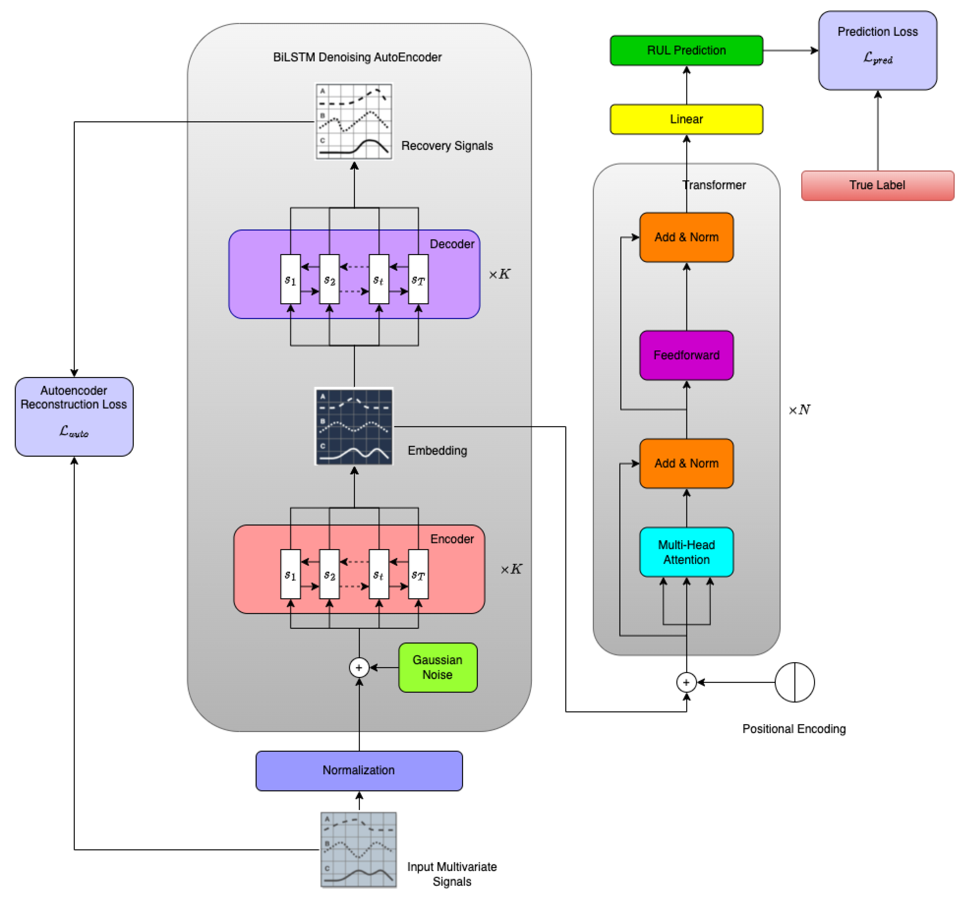
3. Methodology

In this section, we provide a detailed exposition of the overall architecture of our BiLSTM-DAE-based Transformer model. As depicted in Figure 1, our model is composed of two integral components: the BiLSTM autoencoder part and the Transformer part. To facilitate comprehension, we will initially delve into the BiLSTM-DAE part in Section 3.1, followed by a detailed introduction to the Transformer part in Section 3.2.

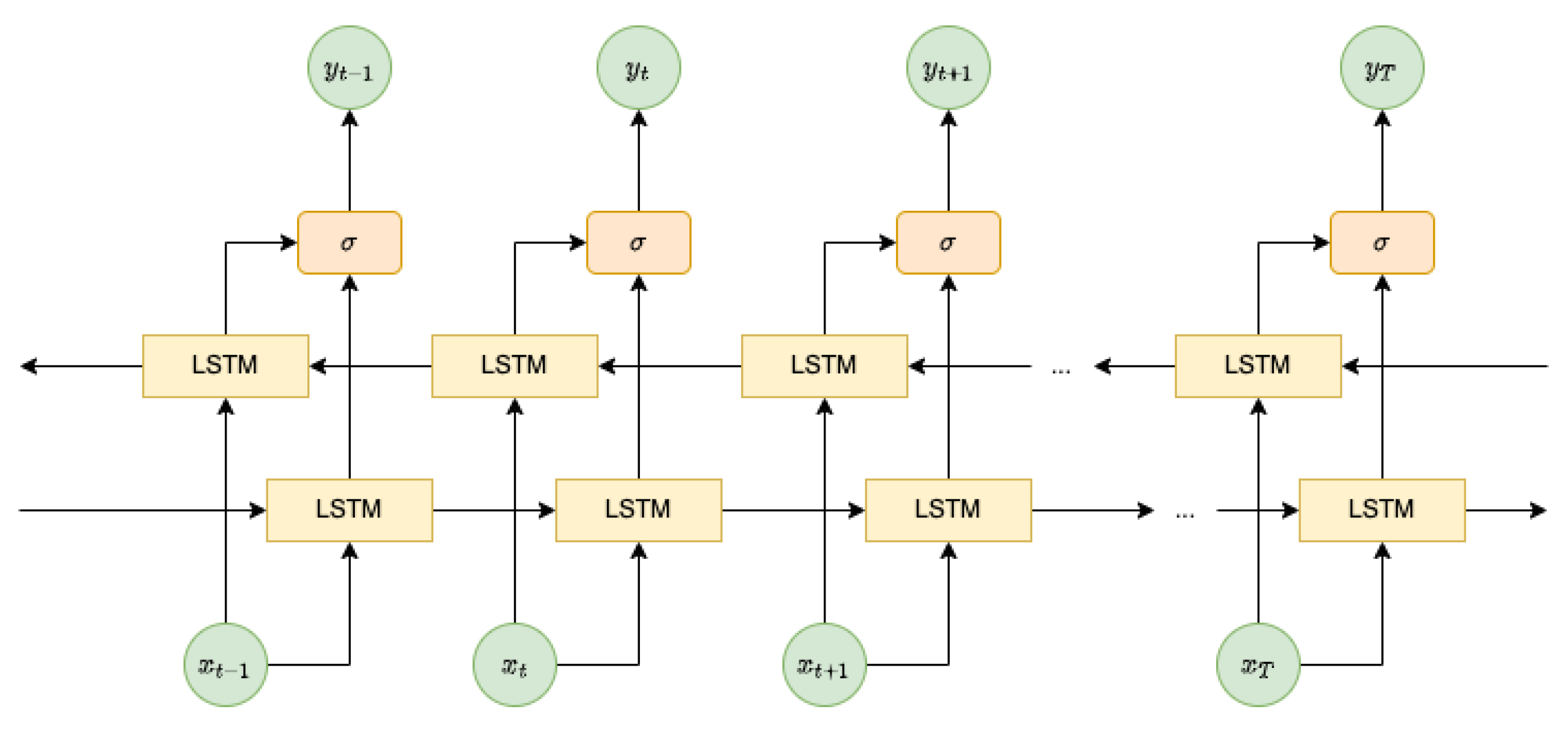
3.1. Bidirectional LSTM Autoencoder

LSTM, a widely employed architecture in time-sequence AI/ML modeling, incorporates gates to regulate information flow in recurrent computations, excelling in the retention of long-term memories. The original LSTM formulation was proposed by Hochreiter and Schmidhuber [49], and the Vanilla LSTM, a popular variant, was introduced in [50], augmenting the LSTM architecture with a forget gate to enhance its capabilities. Figure 2 shows the vanilla LSTM cell.

LSTM memory cells encompass various neural networks referred to as gates, which play a crucial role in managing interactions between memory units, determining what data to retain or discard during training. The input and output gates dictate whether the state memory cells can be modified by incoming signals, while the forget gate governs the decision to retain or erase the preceding signal’s status. In the cell, the functional relationship for each component is given as follows:

$$\left[\begin{array}{c}{f}_t\\ \begin{array}{c}{i}_t\\ {\tilde{C}}_t\\ o_t\end{array}\end{array}\right]=\left[\begin{array}{c}\sigma \\ \begin{array}{c}\sigma \\ \mathrm{t}\mathrm{a}\mathrm{n}\mathrm{h}\\ \sigma \end{array}\end{array}\right]\left(W_{\theta }\left[\begin{array}{c}{X}_t\\ h_{t-1}\end{array}\right]+b_{\theta }\right)$$

(1)

$$C_t=f_t\odot C_{t-1}+i_t\odot {\tilde{C}}_t$$

(2)

$$h_t=o_t\odot \mathrm{t}\mathrm{a}\mathrm{n}\mathrm{h}\left(c_t\right).$$

(3)

The forget gate ($f_t$), input gate ($i_t$), and output gate ($o_t$) are denoted in the LSTM architecture. The forget gate manages the removal of historical information from $C_{t-1}$, while the input and output gates govern the updating and outputting of specific information. The symbol $\sigma$ represents a nonlinear activation function, and the symbol $\odot$ denotes the element-wise product.

BiLSTM, with its bidirectional propagation, processes information in both directions simultaneously, capturing both past and future context. Illustrated in Figure 3, at each time step $\left(t\right)$, the input is fed into both the forward and backward LSTM networks, and the BiLSTM output is a representation of this bidirectional processing.

Denoising autoencoders (DAEs) are a type of artificial neural network used in machine learning for feature learning and data denoising [51]. They are a variant of the traditional autoencoder, which is designed to learn efficient representations of data by training on the corrupted version of the input data. The architecture of a denoising autoencoder typically consists of an encoder and a decoder. The encoder maps the input data to a lower-dimensional representation, and the decoder reconstructs the original data from this representation. During the training process, the network minimizes the reconstruction error, encouraging the model to capture meaningful features while ignoring noise.

Due to the challenges posed by noisy and complex multivariate time-series sensor reading data, we propose the BiLSTM-DAE. Time-series data, especially in multivariate scenarios, often exhibit fluctuations, irregularities, and diverse patterns that can impact the performance of traditional models. The bidirectional nature of the BiLSTM allows it to capture dependencies in both the forward and backward directions, facilitating a more comprehensive understanding of temporal relationships.

Our motivation stems from the need for a robust model that is capable of handling the intricacies of multivariate time-series datasets. The bidirectional architecture enhances the model’s ability to capture temporal dependencies, while the denoising autoencoder aspect improves its resilience against noise and variations in the data. This combined approach aims to provide an effective solution for tasks such as feature extraction, anomaly detection, and prediction within the context of multivariate time-series analysis.

The architecture presented in the left part of Figure 1 focuses on our detailed BiLSTM-DAE model. In this illustration, when provided with a sequence of sensor readings for predicting the RUL of aircraft engines, we initially introduce small Gaussian noises to corrupt the input sequence. The inclusion of Gaussian noise in the training process of an autoencoder serves as implicit regularization, preventing the model from overfitting to the noise present in the input sequence. This, in turn, promotes the development of a more robust feature representation. The corrupted data are then directed into a $K$-layer BiLSTM encoder. The outputs from this BiLSTM encoder are utilized in two distinct ways:

• They are fed into the Transformer component as input data to predict the RUL for aircraft engines;
• They are inputted into the K-layer BiLSTM decoder of the BiLSTM-DAE module to reconstruct the original data before corruption. It is noteworthy that, although the number of layers for the BiLSTM encoder and decoder can differ, we keep them the same in our experiments.

Finally, a reconstruction loss ${(L}_{auto})$ is computed in a conventional autoencoder model to minimize the disparity between the initial input signal$\left(x\right)$ and the reconstructed/recovered signal $\left(\widehat{x}\right)$. In this study, the ${\mathcal{l}}_2$ is employed to measure the difference between $x$ and $\widehat{x}$, as expressed in the following equation:

$$L_{auto}=\frac{1}{N}\sum _{i=1}^N{‖x_i-{\widehat{x}}_i‖}_2.$$

(4)

Here, $N$ denotes the number of sample sequences in our dataset.

3.2. Transformer and Multi-Head Attention

As mentioned earlier, the Transformer architecture has emerged recently as a pivotal paradigm in natural language processing and various sequence-to-sequence tasks. The Transformer architecture relies on self-attention mechanisms, enabling it to capture long-range dependencies in input sequences efficiently [29]. Unlike traditional recurrent or convolutional architectures, the Transformer abandons sequential processing, embracing a parallelizable architecture that facilitates accelerated training on parallel hardware.

At the core of the Transformer’s success is the self-attention mechanism. Given an input sequence, $X=\{x_1,x_2,\dots ,x_n\}$, the self-attention mechanism computes a set of attention weights, allowing each element in the sequence to attend to all other elements. This is achieved through the following formulation:

$$Attention\left(Q,K,V\right)=softmax\left(\frac{Q{K}^T}{\sqrt{d_k}}\right)V.$$

(5)

Here, $Q,K,$ and $V$ denote the query, key, and value matrices, respectively, and $d_k$ represents the dimensionality of the key vectors. The SoftMax operation normalizes the attention scores, determining the weight that each element contributes to the final output.

To enhance the expressive power of self-attention, the Transformer employs a mechanism known as multi-head attention. This involves linearly projecting the input sequences into multiple subspaces, each with its own attention mechanism. The outputs from these multiple heads are then concatenated and linearly transformed to produce the final output. Formally, the multi-head attention is defined as follows:

$$MultiHead\left(Q,K,V\right)=Concat\left(hea{d}^1,hea{d}^2,\dots ,hea{d}^h\right)W_o$$

(6)

where $hea{d}^i=Attention(Q{W}_Q^i,K{W}_k^i,V{W}_V^i)$, and $W_Q^i, W_k^i,W_V^i$ and $W_o$ are all learnable weight matrices.

This multi-head mechanism enables the model to attend to different aspects of the input sequence simultaneously, capturing diverse patterns and dependencies.

Complementing the self-attention mechanism, the Transformer incorporates a feed-forward layer for capturing complex, non-linear relationships within the encoded representations. Each position in the sequence is processed independently through a feed-forward neural network, composed of two linear transformations with an ReLU activation in between:

$$FFN\left(x\right)=ReLU\left(x{W}_1+b_1\right)W_2+b_2.$$

(7)

Here, $W_1,b_1,W_2$, and $b_2$ are learnable parameters. The feed-forward layer introduces additional flexibility, allowing the model to capture intricate patterns and interactions in the data, enhancing its capacity to learn intricate representations.

Finally, as illustrated in the right part of Figure 1, the prediction loss, $L_{pred},$ is computed to minimize the disparity between the predicted RUL $\left(\widehat{y}\right)$ (output of the feed-forward layer) and the true RUL $(y$). In this study, the ${\mathcal{l}}_2$ is employed to measure the difference between $y$ and $\widehat{y}$, as expressed in the following equation:

$$L_{pred}=\frac{1}{N}\sum _{i=1}^N{‖y_i-{\widehat{y}}_i‖}_{2.}$$

(8)

Here, $N$ denotes the number of sample sequences in our dataset.

3.3. Learning

Throughout our training process, our main goal is to acquire meaningful representations of input signals while simultaneously achieving accurate predictions of RUL. The objective function guiding our training encompasses a weighted average of the autoencoder reconstruction loss ($L_{auto})$ and prediction loss ($L_{pred})$. This is formally defined as follows:

$$L=L_{auto}+\alpha \cdot L_{pred}+\lambda \cdot \mathsf{\Omega }\left(\mathsf{\Theta }\right).$$

(9)

Here, $\alpha$ serves as the parameter balancing the weights between the two distinct losses, while $\lambda$ acts as the shrinkage parameter determining regularization strength. The set of parameters in both the BiLSTM-DAE and Transformer networks is denoted by $\mathsf{\Theta }$, and the regularization function $\mathsf{\Omega }(\cdot )$ is employed to prevent model overfitting. In our experimental setup, we opt for the ${\mathcal{l}}_2$ norm to regularize the parameters, $\mathsf{\Theta }$.

4. Experimental Results and Analysis

Our experimentation is carried out on a computing system equipped with an Intel Core i9 3.6 GHz processor, 64 GB of RAM, and an NVIDIA RTX 3080 GPU. The operating system employed is Windows 10, and the programming platform utilized is Python.

In the subsequent subsections of this section, we will commence by introducing the dataset utilized in our study. Following this, we will describe the performance metrics employed for the evaluation of the proposed method. Lastly, we will present our numerical experiments, conduct a comparative analysis of its performance against existing methods, and engage in a comprehensive discussion.

4.1. C-MAPSS Dataset and Preprocessing

The NASA Commercial Modular Aero-Propulsion System Simulation (C-MAPSS) dataset stands as a benchmark in the field, offering a rich source of information for researchers and practitioners engaged in the challenging task of predicting the RUL of turbofan engines [52]. This dataset encompasses simulated sensor data generated by various turbofan engines over time, providing a realistic representation of engine health deterioration. The dataset is structured into four sub-datasets, namely FD001, FD002, FD003, and FD004, with each designed to capture different aspects of engine behavior under various operational conditions and fault scenarios.

The FD001 and FD003 datasets focus on a single operational condition, each containing one and two fault types, respectively. In contrast, the FD002 and FD004 datasets incorporate six distinct operational conditions, along with one and two fault types, respectively. These sub-datasets include detailed information such as engine numbers, serial numbers, configuration items, and sensor data from 21 sensors. See

Table 1. C-MAPSS monitoring sensor data description.

Symbol	Description	Units
T2	Total temperature at fan inlet	R
T24	Total temperature at LPC inlet	R
T30	Total temperature at HPC inlet	R
T50	Total temperature at LPT inlet	R
P2	Pressure at fan inlet	psia
P15	Total pressure in bypass duct	psia
P30	Total pressure at HPC outlet	psia
Nf	Physical fan speed	rpm
Ne	Physical core speed	rpm
epr	Engine pressure ratio	-
Ps30	Static pressure at HPC outlet	psia
Phi	Ratio of fuel flow to Ps30	pps/psi
NRf	Corrected fan speed	rpm
NRe	Corrected core speed	rpm
BPR	Bypass ratio	-
farB	Burner fuel/air ratio	-
htBleed	Bleed Enthalpy	-
Bf-dmd	Demanded fan speed	rpm
PCNfR-dmd	Demanded corrected fan speed	rpm
W31	HPT coolant bleed	lbm/s
W32	LPT coolant bleed	lbm/s

below for a detailed description of these sensors. The sensor data simulate the progressive degradation of the engine, starting from a healthy state and culminating in failure, under diverse initial conditions. Nonetheless, not all sensor data contain information conducive to the estimation of RUL. Certain sensors, for instance, exhibit constant measurements throughout the entire life cycle. To mitigate computational complexity, we adopt the approach outlined in [40], selectively incorporating data from 14 sensors (sensors 2, 3, 4, 7, 8, 9, 11, 12, 13, 14, 15, 17, 20, 21) into our training process.

Recognizing the disparate numerical ranges resulting from distinct sensor measurements, we also employ a min–max normalization technique by using the following formula:

$$x^{\prime }=\frac{x-x_{min }}{x_{max}-x_{min}}.$$

(10)

This normalization procedure serves to standardize the input sensor data, ensuring a consistent and comparable range for all data points.

The training and testing trajectories within each sub-dataset are designed to assess the model’s performance under varying conditions. For instance, FD001 and FD003 consist of 100 training and testing trajectories, while FD002 and FD004 feature 260 and 259 training trajectories and 259 and 248 testing trajectories, respectively. The operational conditions and fault modes further contribute to the dataset’s complexity, making it a suitable benchmark for evaluating the effectiveness of predictive models.

Table 2. Parameters of the C-MAPSS dataset.

Dataset	FD001	FD002	FD003	FD004
No. of Training Trajectories	100	260	100	249
No. of Testing Trajectories	100	259	100	248
Operating Conditions	1	6	1	6
Fault Modes	1	1	2	2

summarizes the key statistics for the C-MAPSS dataset.

The training set spans the entire operational lifecycle of the turbofan engine, capturing data from its initial operation to degradation and failure. Conversely, the test set begins at a healthy state and undergoes arbitrary truncation, with the operating time periods leading up to system failure calculated from these truncated data. Additionally, the test set includes the actual RUL values of the test engine, facilitating the assessment of the model’s accuracy in predicting the time remaining until failure.

In light of the challenges associated with RUL labeling in run-to-fail sequences, our approach diverges from earlier methodologies, such as the linear decrease assumption in a previous study [53]. This assumption posits that RULs decrease linearly over time, implying a linear development of the system’s degradation state. However, this assumption may not accurately reflect the reality of system degradation, especially during the initial stages of its life cycle when degradation is typically negligible.

To address this, we adopt a more nuanced RUL labeling strategy inspired by the truncated linear model [27]. This approach recognizes that the system experiences varying degrees of degradation over different phases of its life cycle. In Figure 4, our labeling procedure is visually represented. Initially, RULs are labeled with a constant value, denoted as $RU{L}_{max}$, akin to the horizon dot line. As the system operates over time, it transitions into a phase of linear degradation until it ultimately reaches failure. This truncated linear model provides a more realistic representation of RUL evolution, accommodating the dynamic nature of system degradation. By assigning RUL labels that consider both the initial phase of system operation and subsequent linear degradation periods, our approach captures the nuanced progression of system health over time. This ensures that our RUL labeling aligns more closely with the actual behavior of the turbofan engines in the dataset.

.

4.2. Evaluation Metrics

Two evaluation metrics used to evaluate the prediction performance of RUL include the root mean squared error (RMSE) and Score, which are defined as follows:

$$RMSE=\sqrt{\frac{\sum _{i=1}^n{\left(y_i-{\widehat{y}}_i\right)}^2}{N}}$$

(11)

$$Score=\left\{\begin{array}{c}{\displaystyle \sum _{i=1}^N}{e}^{-\left(\frac{y_i-{\widehat{y}}_i}{13}\right)}-1, d<0\\ {\displaystyle \sum _{i=1}^N}{e}^{-\left(\frac{y_i-{\widehat{y}}_i}{10}\right)}-1, d\ge 0\end{array}\right..$$

(12)

With an increase in the absolute value of $y_i-{\widehat{y}}_i$, both evaluation indices show an upward trend. Notably, when $y_i-{\widehat{y}}_i>0$, the Score metric introduces distinct penalty weights for model predictions’ lag and advancement. In cases where the predicted value is smaller than the true value, indicating prediction advancement, the penalty coefficient is correspondingly smaller. Conversely, if the prediction lags, the consequences are deemed more severe, leading to a larger penalty coefficient. Anticipating the RUL value earlier facilitates proactive maintenance planning, mitigating potential losses and underscoring the importance of the penalty coefficient’s dynamic adjustment based on the direction of prediction deviation.

4.3. RUL Prediction

To verify the performance of the proposed BiLSTM-DAE Transformer model, we compare our model with other existing RUL prediction methods, including the multi-layer perceptron (MLP) [54], support vector regression (SVR) [54], CNNs [54], LSTM [27], BiLSTM [55], the deep belief network ensemble (DBNE) [56], B-LSTM [23], the gated convolutional Transformer (GCT) [40], CNN + LSTM [57], multi-head CNN + LSTM [58], and DAST [42].

Table 3. Performance comparison. The bold number represents the best model, while the underscore number represents the second-best model.

Method	FD001		FD002		FD003		FD004
	RMSE	Score	RMSE	Score	RMSE	Score	RMSE	Score
MLP	37.56	18,000	80.03	7,800,000	37.39	17,400	77.37	5,620,000
SVR	20.96	1380	42.00	590,000	21.05	1600	45.35	371,000
CNN	18.45	1290	30.29	13,600	19.82	1600	29.16	7890
LSTM	16.14	338	24.49	4450	16.18	852	28.17	5550
BiLSTM	13.65	295	23.18	4130	13.74	317	24.86	5430
DBNE	17.27	523	37.28	49,800	18.47	574	30.96	12,100
B-LSTM	12.45	279	15.36	4250	13.37	356	16.24	5220
GCT	11.27	-	22.81	-	11.42	-	24.86	-
CNN + LSTM	16.16	303	20.44	3440	17.12	1420	23.25	4630
DAST	11.43	203	15.25	924.96	11.32	154	18.36	1490
Multi-head CNN + LSTM	12.19	259	19.93	4350	12.85	343	22.89	4340
Proposed Method	10.98	186	16.12	2937	11.14	252	18.15	3840

shows the comparison results.

As depicted in Table 3, our BiLSTM-DAE-Transformer architecture exhibits superior performance on both the FD001 and FD003 datasets, showcasing relative improvements in RMSE compared to previous state-of-the-art models. Specifically, the relative improvements range from 0.28 for FD003 to 0.29 for FD001 in terms of the RMSE. Additionally, our model secures the second-best performance on the FD002 and FD004 datasets, emphasizing its effectiveness across different operational conditions. Notably, our model achieves the smallest Score across all four datasets in comparison to existing methods. Particularly noteworthy are the substantial Score improvements for FD001 and FD003, where our model outperforms state-of-the-art models by 28% and 26%, respectively. In contrast to other autoencoder methods that involve building the autoencoder and prediction model separately, our end-to-end approach requires less effort in implementation. This advantage stems from the seamless integration of the autoencoder and prediction model within our architecture. The end-to-end nature of our method streamlines the implementation process, making it more efficient and requiring fewer resources.

To further substantiate the reliability of our model, we conduct a comparative analysis by visually contrasting the estimated RUL with the ground-truth RULs, presenting the results in Figure 5. This visual representation offers a comprehensive understanding of the accuracy and effectiveness of our RUL predictions across diverse datasets.

To enhance clarity in our analysis, we organize all test sequences based on their corresponding ground-truth RUL lengths along the horizon axis in ascending order. Upon reviewing Figure 5, it becomes evident that our model consistently produces satisfactory outcomes. Notably, in the case of FD001 and FD003, our model demonstrates accurate RUL predictions in both the early and late stages of the engine life cycle, with relatively smaller variations. Conversely, for the FD002 and FD004 datasets, predictions appear noisier at the early and late stages compared to FD001 and FD003. We attribute this variability to differences in the complexity of working conditions, as characterized by the number of operational conditions and fault modes, and the size of the training dataset.

As indicated in Table 2, FD001 training samples are derived from a single working condition, offering a simpler scenario for training. Similarly, FD003 involves two working conditions. In contrast, FD002 and FD004 present more intricate scenarios with six and twelve working conditions, respectively (comprising six operational conditions and one or two fault modes). This increased complexity in FD002 and FD004 can contribute to the noisier predictions observed, accentuating the impact of working condition intricacies and training dataset size on the model’s performance across different datasets.

4.4. Ablation Study

In our paper, we developed a BiLSTM-DAE-Transformer model that integrates a Transformer and denoising autoencoder for predicting RUL. In this subsection, we perform ablation study experiments to examine the influence of each component in our proposed model. Specifically, we compare the prediction performances, measured in terms of RMSE, for the following models on the FD001 dataset:

• BiLSTM-DAE-Transformer: The proposed model that integrates the Transformer encoder and BiLSTM DAE;
• BiLSTM-DAE-Transformer-Noise: The proposed model that integrates the Transformer encoder and BiLSTM DAE with noisy input (original sensor readings plus small Gaussian noise);
• BiLSTM-DAE-LSTM: The model that integrates LSTM and BiLSTM DAE;
• BiLSTM-AE-Transformer: The proposed model without adding noise for DAE training;
• Transformer: The model with only a Transformer encoder for RUL prediction, and without any DAEs;
• LSTM: The model with only LSTM for RUL prediction, and without any DAEs.

The results in

Table 4. Ablation study of the proposed BiLSTM-DAE-Transformer architecture on the FD001 dataset.

Model	RMSE	Difference
BiLSTM-DAE-Transformer	10.98	-
BiLSTM-DAE-Transformer-Noise	11.31	0.33
BiLSTM-DAE-LSTM	15.24	4.26
BiLSTM-AE-Transformer	12.44	1.46
Transformer	13.02	2.04
LSTM	16.14	5.16

highlight the significance of each component in our proposed BiLSTM-DAE-Transformer model for achieving robust prediction performance:

• The comparison between BiLSTM-DAE-Transformer and BiLSTM-DAE-LSTM demonstrates that the Transformer architecture contributes to superior prediction performance, attributed to its ability to handle long sequences more effectively than LSTM;
• The comparison in prediction results between BiLSTM-DAE-Transformer and BiLSTM-AE-Transformer underscores the importance of the denoising autoencoder in our framework. The introduction of noise during DAE training enhances the robustness of feature representation;
• The comparison between BiLSTM-DAE-Transformer and the Transformer emphasizes the significance of the autoencoder component in our framework. The autoencoder embeds valuable information into a lower-dimensional space, facilitating Transformer architectures in capturing temporal structures within sequence data more efficiently;
• The contrast between BiLSTM-DAE-Transformer and BiLSTM-DAE-Transformer-Noise demonstrates the robust performance of our proposed model, even in the presence of contaminated sensor readings.

5. Conclusions

This paper presents a novel and effective approach for RUL prediction in turbofan engines using a hybrid architecture comprising bidirectional LSTM, denoising autoencoder, and Transformer models. Leveraging the C-MAPSS dataset, we demonstrated the superior performance of our BiLSTM-DAE-Transformer architecture compared to state-of-the-art models across multiple datasets. Our truncated RUL strategy for RUL labeling and the incorporation of a selective set of 14 sensors significantly contribute to the success of our model. The end-to-end nature of our approach simplifies implementation compared to alternative autoencoder-based methods, where the autoencoder and prediction model are built separately. The visual validation of our model against ground-truth RULs showcases its accuracy and reliability, particularly in the early and late stages of engine life cycles. Notably, our model outperforms existing methods, achieving substantial improvements in Score and RMSE. These results underscore the practical applicability of our proposed approach in turbofan engine prognostics, enabling more accurate maintenance planning and the avoidance of unplanned system shutdowns.

While the proposed methods exhibit superior performance in predicting RUL, they encounter challenges in handling variable lengths of different sensor inputs and managing missing data in the dataset. Future endeavors should focus on exploring methods to address these issues. Another limitation of the proposed method pertains to its interpretability; it lacks the capability to offer explanations for why the model considers the equipment to be nearing failure. Hence, incorporating explainable artificial intelligence (XAI) methods like SHAP and LIME could be intriguing to comprehend the prediction logic of the model. Moreover, there is room for further improvements to address additional complexities and diverse operational scenarios, enhancing the precision and versatility of our RUL prediction model. A promising avenue for investigation involves investigating the generalization capacity of the proposed BiLSTM-DAE-Transformer model on alternative RUL prediction datasets, including those related to batteries and rolling bearings.

References

1. Fan, Z.; Chang, K.; Ji, R.; Chen, G. Data Fusion for Optimal Condition-Based Aircraft Fleet Maintenance with Predictive Analytics. J. Adv. Inf. Fusion 2023, in press. [Google Scholar]
2. Giantomassi, A.; Ferracuti, F.; Benini, A.; Ippoliti, G.; Longhi, S.; Petrucci, A. Hidden Markov Model for Health Estimation and Prognosis of Turbofan Engines. In Proceedings of the ASME 2011 International Design Engineering Technical Conferences and Computers and Information in Engineering Conference, Washington, DC, USA, 28–31 August 2011; pp. 681–689. [Google Scholar]
3. Lin, J.; Liao, G.; Chen, M.; Yin, H. Two-Phase Degradation Modeling and Remaining Useful Life Prediction Using Nonlinear Wiener Process. Comput. Ind. Eng. 2021, 160, 107533. [Google Scholar] [CrossRef]
4. Yu, W.; Tu, W.; Kim, I.Y.; Mechefske, C. A Nonlinear-Drift-Driven Wiener Process Model for Remaining Useful Life Estimation Considering Three Sources of Variability. Reliab. Eng. Syst. Saf. 2021, 212, 107631. [Google Scholar] [CrossRef]
5. Feng, D.; Xiao, M.; Liu, Y.; Song, H.; Yang, Z.; Zhang, L. A Kernel Principal Component Analysis–Based Degradation Model and Remaining Useful Life Estimation for the Turbofan Engine. Adv. Mech. Eng. 2016, 8, 1687814016650169. [Google Scholar] [CrossRef]
6. Lv, Y.; Zheng, P.; Yuan, J.; Cao, X. A Predictive Maintenance Strategy for Multi-Component Systems Based on Components’ Remaining Useful Life Prediction. Mathematics 2023, 11, 3884. [Google Scholar] [CrossRef]
7. Zhang, Y.; Guo, G.; Yang, F.; Zheng, Y.; Zhai, F. Prediction of Tool Remaining Useful Life Based on NHPP-WPHM. Mathematics 2023, 11, 1837. [Google Scholar] [CrossRef]
8. Si, X.-S.; Wang, W.; Hu, C.-H.; Zhou, D.-H. Remaining Useful Life Estimation—A Review on the Statistical Data Driven Approaches. Eur. J. Oper. Res. 2011, 213, 1–14. [Google Scholar] [CrossRef]
9. Li, W.; Lee, J.; Purl, J.; Greitzer, F.; Yousefi, B.; Laskey, K. Experimental Investigation of Demographic Factors Related to Phishing Susceptibility; University of Hawaii Manoa Library: Honolulu, HI, USA, 2020; ISBN 978-0-9981331-3-3. [Google Scholar]
10. Greitzer, F.L.; Li, W.; Laskey, K.B.; Lee, J.; Purl, J. Experimental Investigation of Technical and Human Factors Related to Phishing Susceptibility. ACM Trans. Soc. Comput. 2021, 4, 8:1–8:48. [Google Scholar] [CrossRef]
11. Li, W.; Finsa, M.M.; Laskey, K.B.; Houser, P.; Douglas-Bate, R. Groundwater Level Prediction with Machine Learning to Support Sustainable Irrigation in Water Scarcity Regions. Water 2023, 15, 3473. [Google Scholar] [CrossRef]
12. Liu, W.; Zou, P.; Jiang, D.; Quan, X.; Dai, H. Computing River Discharge Using Water Surface Elevation Based on Deep Learning Networks. Water 2023, 15, 3759. [Google Scholar] [CrossRef]
13. Fan, Z.; Chang, K.; Raz, A.K.; Harvey, A.; Chen, G. Sensor Tasking for Space Situation Awareness: Combining Reinforcement Learning and Causality. In Proceedings of the 2023 IEEE Aerospace Conference, Big Sky, MT, USA, 4–11 March 2023; pp. 1–9. [Google Scholar]
14. Salmaso, F.; Trisolini, M.; Colombo, C. A Machine Learning and Feature Engineering Approach for the Prediction of the Uncontrolled Re-Entry of Space Objects. Aerospace 2023, 10, 297. [Google Scholar] [CrossRef]
15. Zhou, W. Condition State-Based Decision Making in Evolving Systems: Applications in Asset Management and Delivery. Ph.D. Thesis, George Mason University, Fairfax, VA, USA, 2023. [Google Scholar]
16. Ravi, C.; Tigga, A.; Reddy, G.T.; Hakak, S.; Alazab, M. Driver Identification Using Optimized Deep Learning Model in Smart Transportation. ACM Trans. Internet Technol. 2022, 22, 84:1–84:17. [Google Scholar] [CrossRef]
17. Ordóñez, C.; Sánchez Lasheras, F.; Roca-Pardiñas, J.; de Cos Juez, F.J. A Hybrid ARIMA–SVM Model for the Study of the Remaining Useful Life of Aircraft Engines. J. Comput. Appl. Math. 2019, 346, 184–191. [Google Scholar] [CrossRef]
18. García Nieto, P.J.; García-Gonzalo, E.; Sánchez Lasheras, F.; de Cos Juez, F.J. Hybrid PSO–SVM-Based Method for Forecasting of the Remaining Useful Life for Aircraft Engines and Evaluation of Its Reliability. Reliab. Eng. Syst. Saf. 2015, 138, 219–231. [Google Scholar] [CrossRef]
19. Benkedjouh, T.; Medjaher, K.; Zerhouni, N.; Rechak, S. Health Assessment and Life Prediction of Cutting Tools Based on Support Vector Regression. J. Intell. Manuf. 2015, 26, 213–223. [Google Scholar] [CrossRef]
20. Wang, H.; Li, D.; Li, D.; Liu, C.; Yang, X.; Zhu, G. Remaining Useful Life Prediction of Aircraft Turbofan Engine Based on Random Forest Feature Selection and Multi-Layer Perceptron. Appl. Sci. 2023, 13, 7186. [Google Scholar] [CrossRef]
21. Wang, Q.; Zheng, S.; Farahat, A.; Serita, S.; Gupta, C. Remaining Useful Life Estimation Using Functional Data Analysis. In Proceedings of the 2019 IEEE International Conference on Prognostics and Health Management (ICPHM), San Francisco, CA, USA, 17–20 June 2019; pp. 1–8. [Google Scholar]
22. Rao, A.R.; Wang, H.; Gupta, C. Functional Approach for Two Way Dimension Reduction in Time Series. In Proceedings of the 2022 IEEE International Conference on Big Data (Big Data), Osaka, Japan, 17–20 December 2022; pp. 1099–1106. [Google Scholar]
23. Wang, X.; Huang, T.; Zhu, K.; Zhao, X. LSTM-Based Broad Learning System for Remaining Useful Life Prediction. Mathematics 2022, 10, 2066. [Google Scholar] [CrossRef]
24. Ensarioğlu, K.; İnkaya, T.; Emel, E. Remaining Useful Life Estimation of Turbofan Engines with Deep Learning Using Change-Point Detection Based Labeling and Feature Engineering. Appl. Sci. 2023, 13, 11893. [Google Scholar] [CrossRef]
25. Yuan, M.; Wu, Y.; Lin, L. Fault Diagnosis and Remaining Useful Life Estimation of Aero Engine Using LSTM Neural Network. In Proceedings of the 2016 IEEE International Conference on Aircraft Utility Systems (AUS), Beijing, China, 10–12 October 2016; pp. 135–140. [Google Scholar]
26. Wu, Y.; Yuan, M.; Dong, S.; Lin, L.; Liu, Y. Remaining Useful Life Estimation of Engineered Systems Using Vanilla LSTM Neural Networks. Neurocomputing 2018, 275, 167–179. [Google Scholar] [CrossRef]
27. Zheng, S.; Ristovski, K.; Farahat, A.; Gupta, C. Long Short-Term Memory Network for Remaining Useful Life Estimation. In Proceedings of the 2017 IEEE International Conference on Prognostics and Health Management (ICPHM), Dallas, TX, USA, 19–21 June 2017; pp. 88–95. [Google Scholar]
28. Li, X.; Ding, Q.; Sun, J.-Q. Remaining Useful Life Estimation in Prognostics Using Deep Convolution Neural Networks. Reliab. Eng. Syst. Saf. 2018, 172, 1–11. [Google Scholar] [CrossRef]
29. Yu, W.; Kim, I.Y.; Mechefske, C. Remaining Useful Life Estimation Using a Bidirectional Recurrent Neural Network Based Autoencoder Scheme. Mech. Syst. Signal Process. 2019, 129, 764–780. [Google Scholar] [CrossRef]
30. Zhao, C.; Huang, X.; Li, Y.; Yousaf Iqbal, M. A Double-Channel Hybrid Deep Neural Network Based on CNN and BiLSTM for Remaining Useful Life Prediction. Sensors 2020, 20, 7109. [Google Scholar] [CrossRef] [PubMed]
31. Peng, C.; Wu, J.; Wang, Q.; Gui, W.; Tang, Z. Remaining Useful Life Prediction Using Dual-Channel LSTM with Time Feature and Its Difference. Entropy 2022, 24, 1818. [Google Scholar] [CrossRef] [PubMed]
32. Wang, Y.; Zhao, Y. Multi-Scale Remaining Useful Life Prediction Using Long Short-Term Memory. Sustainability 2022, 14, 15667. [Google Scholar] [CrossRef]
33. Lyu, Y.; Zhang, Q.; Wen, Z.; Chen, A. Remaining Useful Life Prediction Based on Multi-Representation Domain Adaptation. Mathematics 2022, 10, 4647. [Google Scholar] [CrossRef]
34. Deng, F.; Bi, Y.; Liu, Y.; Yang, S. Deep-Learning-Based Remaining Useful Life Prediction Based on a Multi-Scale Dilated Convolution Network. Mathematics 2021, 9, 3035. [Google Scholar] [CrossRef]
35. Zhou, J.; Qin, Y.; Luo, J.; Wang, S.; Zhu, T. Dual-Thread Gated Recurrent Unit for Gear Remaining Useful Life Prediction. IEEE Trans. Ind. Inform. 2023, 19, 8307–8318. [Google Scholar] [CrossRef]
36. Zhuang, L.; Xu, A.; Wang, X.-L. A Prognostic Driven Predictive Maintenance Framework Based on Bayesian Deep Learning. Reliab. Eng. Syst. Saf. 2023, 234, 109181. [Google Scholar] [CrossRef]
37. Ding, A.; Qin, Y.; Wang, B.; Cheng, X.; Jia, L. An Elastic Expandable Fault Diagnosis Method of Three-Phase Motors Using Continual Learning for Class-Added Sample Accumulations. IEEE Trans. Ind. Electron. 2023, 1–10. [Google Scholar] [CrossRef]
38. Vaswani, A.; Shazeer, N.; Parmar, N.; Uszkoreit, J.; Jones, L.; Gomez, A.N.; Kaiser, Ł.; Polosukhin, I. Attention Is All You Need. In Proceedings of the Advances in Neural Information Processing Systems, Long Beach, CA, USA, 4–9 December 2017; Curran Associates, Inc.: Sydney, Australia, 2017; Volume 30. [Google Scholar]
39. Dosovitskiy, A.; Beyer, L.; Kolesnikov, A.; Weissenborn, D.; Zhai, X.; Unterthiner, T.; Dehghani, M.; Minderer, M.; Heigold, G.; Gelly, S.; et al. An Image Is Worth 16x16 Words: Transformers for Image Recognition at Scale. arXiv 2020, arXiv:2010.11929. [Google Scholar]
40. Mo, Y.; Wu, Q.; Li, X.; Huang, B. Remaining Useful Life Estimation via Transformer Encoder Enhanced by a Gated Convolutional Unit. J. Intell. Manuf. 2021, 32, 1997–2006. [Google Scholar] [CrossRef]
41. Ai, S.; Song, J.; Cai, G. Sequence-to-Sequence Remaining Useful Life Prediction of the Highly Maneuverable Unmanned Aerial Vehicle: A Multilevel Fusion Transformer Network Solution. Mathematics 2022, 10, 1733. [Google Scholar] [CrossRef]
42. Zhang, Z.; Song, W.; Li, Q. Dual-Aspect Self-Attention Based on Transformer for Remaining Useful Life Prediction. IEEE Trans. Instrum. Meas. 2022, 71, 2505711. [Google Scholar] [CrossRef]
43. Hu, Q.; Zhao, Y.; Ren, L. Novel Transformer-Based Fusion Models for Aero-Engine Remaining Useful Life Estimation. IEEE Access 2023, 11, 52668–52685. [Google Scholar] [CrossRef]
44. Li, X.; Li, J.; Zuo, L.; Zhu, L.; Shen, H.T. Domain Adaptive Remaining Useful Life Prediction With Transformer. IEEE Trans. Instrum. Meas. 2022, 71, 3521213. [Google Scholar] [CrossRef]
45. Ding, Y.; Jia, M. Convolutional Transformer: An Enhanced Attention Mechanism Architecture for Remaining Useful Life Estimation of Bearings. IEEE Trans. Instrum. Meas. 2022, 71, 3515010. [Google Scholar] [CrossRef]
46. Chadha, G.S.; Shah, S.R.B.; Schwung, A.; Ding, S.X. Shared Temporal Attention Transformer for Remaining Useful Lifetime Estimation. IEEE Access 2022, 10, 74244–74258. [Google Scholar] [CrossRef]
47. Zhang, Y.; Su, C.; Wu, J.; Liu, H.; Xie, M. Trend-Augmented and Temporal-Featured Transformer Network with Multi-Sensor Signals for Remaining Useful Life Prediction. Reliab. Eng. Syst. Saf. 2024, 241, 109662. [Google Scholar] [CrossRef]
48. Chen, D.; Hong, W.; Zhou, X. Transformer Network for Remaining Useful Life Prediction of Lithium-Ion Batteries. IEEE Access 2022, 10, 19621–19628. [Google Scholar] [CrossRef]
49. Hochreiter, S.; Schmidhuber, J. Long Short-Term Memory. Neural Comput. 1997, 9, 1735–1780. [Google Scholar] [CrossRef]
50. Gers, F.A.; Schmidhuber, J.; Cummins, F. Learning to Forget: Continual Prediction with LSTM. Neural Comput. 2000, 12, 2451–2471. [Google Scholar] [CrossRef] [PubMed]
51. Vincent, P.; Larochelle, H.; Bengio, Y.; Manzagol, P.-A. Extracting and Composing Robust Features with Denoising Autoencoders. In Proceedings of the 25th International Conference on Machine Learning, New York, NY, USA, 5–9 July 2008; Association for Computing Machinery: New York, NY, USA; pp. 1096–1103. [Google Scholar]
52. Saxena, A.; Goebel, K.; Simon, D.; Eklund, N. Damage Propagation Modeling for Aircraft Engine Run-to-Failure Simulation. In Proceedings of the 2008 International Conference on Prognostics and Health Management, Evanston, IL, USA, 7–10 October 2008; pp. 1–9. [Google Scholar]
53. Wu, Q.; Ding, K.; Huang, B. Approach for Fault Prognosis Using Recurrent Neural Network. J. Intell. Manuf. 2020, 31, 1621–1633. [Google Scholar] [CrossRef]
54. Sateesh Babu, G.; Zhao, P.; Li, X.-L. Deep Convolutional Neural Network Based Regression Approach for Estimation of Remaining Useful Life. In Database Systems for Advanced Applications; Navathe, S.B., Wu, W., Shekhar, S., Du, X., Wang, X.S., Xiong, H., Eds.; Springer International Publishing: Cham, Switzerland, 2016; pp. 214–228. [Google Scholar]
55. Wang, J.; Wen, G.; Yang, S.; Liu, Y. Remaining Useful Life Estimation in Prognostics Using Deep Bidirectional LSTM Neural Network. In Proceedings of the 2018 Prognostics and System Health Management Conference (PHM-Chongqing), Chongqing, China, 26–28 October 2018; pp. 1037–1042. [Google Scholar]
56. Zhang, C.; Lim, P.; Qin, A.K.; Tan, K.C. Multiobjective Deep Belief Networks Ensemble for Remaining Useful Life Estimation in Prognostics. IEEE Trans. Neural Netw. Learn. Syst. 2017, 28, 2306–2318. [Google Scholar] [CrossRef] [PubMed]
57. Kong, Z.; Cui, Y.; Xia, Z.; Lv, H. Convolution and Long Short-Term Memory Hybrid Deep Neural Networks for Remaining Useful Life Prognostics. Appl. Sci. 2019, 9, 4156. [Google Scholar] [CrossRef]
58. Mo, H.; Lucca, F.; Malacarne, J.; Iacca, G. Multi-Head CNN-LSTM with Prediction Error Analysis for Remaining Useful Life Prediction. In Proceedings of the 2020 27th Conference of Open Innovations Association (FRUCT), Trento, Italy, 7–9 September 2020; pp. 164–171. [Google Scholar]
Figure 1. Overall structure of BiLSTM-DAE Transformer model.
Mathematics 11 04972 g001
Figure 2. A vanilla LSTM cell.
Mathematics 11 04972 g002
Figure 3. BiLSTM architecture.
Mathematics 11 04972 g003
Figure 4. Truncated RUL of C-MAPSS dataset, R U L m a x = 130 .
Mathematics 11 04972 g004
Figure 5. Comparisons between predicted RUL and ground-truth RUL for all four C-MAPSS datasets. The x-axis in the figures corresponds to the engine unit index, while the y-axis represents the remaining useful life. (a) RUL prediction for FD001; (b) RUL prediction for FD002; (c) RUL prediction for FD003; (d) RUL prediction for FD004.
Mathematics 11 04972 g005