Article

Empiric Solutions to Full Fuzzy Linear Programming Problems Using the Generalized “min” Operator

by
Bogdana Stanojević
1 and
Sorin Nǎdǎban
2,*
1
Mathematical Institute of the Serbian Academy of Sciences and Arts, 11000 Belgrade, Serbia
2
Department of Mathematics and Computer Science, Aurel Vlaicu University of Arad, RO-310330 Arad, Romania
*
Author to whom correspondence should be addressed.
Mathematics 2023, 11(23), 4864; https://doi.org/10.3390/math11234864
Submission received: 24 October 2023 / Revised: 17 November 2023 / Accepted: 1 December 2023 / Published: 4 December 2023
(This article belongs to the Special Issue Fuzzy Logic and Soft Computing—In Memory of Lotfi A. Zadeh)

Abstract

:
Solving optimization problems in a fuzzy environment is an area widely addressed in the recent literature. De-fuzzification of data, construction of crisp more or less equivalent problems, unification of multiple objectives, and solving a single crisp optimization problem are the general descriptions of many procedures that approach fuzzy optimization problems. Such procedures are misleading (since relevant information is lost through de-fuzzyfication and aggregation of more objectives into a single one), but they are still dominant in the literature due to their simplicity. In this paper, we address the full fuzzy linear programming problem, and provide solutions in full accordance with the extension principle. The main contribution of this paper is in modeling the conjunction of the fuzzy sets using the “product” operator instead of “min” within the definition of the solution concept. Our theoretical findings show that using a generalized “min” operator within the extension principle assures thinner shapes to the derived fuzzy solutions compared to those available in the literature. Thinner shapes are always desirable, since such solutions provide the decision maker with more significant information.

1. Introduction

The modeling of uncertainty will always be an open issue. The trade off between model simplicity and accuracy is an issue that is addressed in different ways in different research fields. As pointed out in [1], more realistic data representations are desired nowadays, since the complexity of decision-making contexts is steadily growing. Guerra et al. [2] explained that, generally, a complete investigation of an observed fuzzy system can be carried out by using fuzzy computing combined with an appropriate sensitive analysis technique, based on the application of the extension principle (EP).
The basic idea of this paper is to introduce a new solution approach to fuzzy optimization problems that is able to derive thinner shapes to the fuzzy set solutions. Such shapes are highly desired in the decision-making process in fuzzy environments.
In the recent literature [3], the importance of reconsidering the position of the EP within fuzzy optimization was emphasized, and novel research directions were suggested. New methodologies developed in full accordance with the extension principle were proposed to solve linear (LP) and linear fractional programming problems with fuzzy numbers. For all these approaches, the operators used to aggregate the membership functions of the fuzzy quantities, define the optimal solution concept, and formulate the membership functions of the optimal results were min and max. They were used to intersect and unite the involved fuzzy sets, respectively.
The main contribution of this paper is in modeling the conjunction of the fuzzy sets using another operator than the min operator, namely any generalized product, within the definition of the solution concept to full fuzzy linear programming (FF-LP) problems. The term full fuzzy optimization problem is used whenever both the parameters and variables of an optimization problem are expressed by fuzzy quantities. We formulate a solution approach based on a chosen operator of a generalized product that empirically derives the fuzzy set representing the optimal value of the objective function still in accordance to the extension principle. To illustrate our novel approach, we use two numerical examples: the first one is recalled from Wang and Peng [4] and has parameters described by trapezoidal fuzzy numbers, while the second one is taken from Ezzati et al. [5] and uses triangular fuzzy numbers to describe its parameters.
Ezzati et al. [5] provided a solution approach to FF-LP based on multiple objective optimization. They applied fuzzy arithmetic on the problem’s parameters, and constructed a triangular fuzzy value of the objective function considering that the decision variables are also triangular fuzzy numbers. Then, using a lexicographic method, they derived the compromise objective values to the three crisp objectives that are the components of the previously obtained triangular fuzzy number. As proven in [6], the solution derived in this manner is not in accordance with the extension principle, since fuzzy arithmetic and fuzzy optimization were performed in two sequential steps.
Wang and Peng [4] proposed a methodology to derive a numerical description of the membership function of the optimal fuzzy value of the objective function. Their approach was based on the extension principle and min operator for fuzzy sets conjunction, but they introduced some approximations to reduce the numerical complexity. In addition, they mentioned that their approach cannot disclose the shapes of the optimal fuzzy solutions. Their results were expanded in [7], where analytic descriptions of fuzzy sets representing the optimal values and solutions were proposed via a parametric analysis of the optimal solutions to certain crisp linear optimization problems.
Similar studies that use max–min operators within the extension principle applied to linear and linear fractional transportation problems can be found in the literature, see, for instance, [8,9,10,11,12,13,14,15,16]. Another related area is Data Enveloped Analysis (DEA) in fuzzy environments. To date, methodologies that use the extension principle and are part of fuzzy DEA work with max–min operators. For more details, we refer the reader to [17,18,19,20]. All these papers can be of interest for further research on substituting the min operator with the generalized product within the EP in order to obtain fuzzy set results with narrower shapes.
Methodologies that do not comply with the extension principle are generally misleading, since significant information might be lost through the de-fuzzyfication process and other simplistic operations. Recently, Sotoudeh-Anvari [21] reviewed the papers published between 2010 and 2020 containing theoretical weaknesses and mathematically incorrect assumptions related to fuzzy operations research. Ghanbari et al. [22] reviewed the recent literature on fuzzy linear programming, presenting various models and their corresponding solution approaches.
The literature review linked to full fuzzy mathematical programming is briefly summarized in Table 1.
The rest of the paper is organized as follows: Section 2 provides preliminary definitions needed to establish the context of our study and, in Section 3, we formulate the problem we address and present our novel optimization approach based on the extension principle and the generalized product operator. We report our numerical results in Section 4 and compare them with the results found in the literature in Section 5. The final conclusions and directions for further research are provided in Section 6.

2. Preliminaries

2.1. Fuzzy Sets and Fuzzy Numbers

Fuzzy sets were introduced in [23] by Zadeh, aiming to provide a tool for modeling uncertainty. The concept of fuzzy sets has been widely applied and has influenced a lot of scientific fields. Shi [24] predicted a continuous growth in the applicability of fuzzy sets and fuzzy logic in science, mathematics and society.
The fuzzy set A ˜ over the universe X is a collection of pairs x , μ A ˜ x , where x X and μ A ˜ x 0 , 1 . The function μ A ˜ : X 0 , 1 is called the membership function of the fuzzy set A ˜ , and μ A ˜ x is the membership degree of the element x in A ˜ .
The crisp set
Supp A ˜ = x X | μ A ˜ x > 0
represents the support of the fuzzy set A ˜ , and contains all elements x with non-zero membership degree.
The α -cut of a fuzzy set A ˜ is denoted by A ˜ α , and it is defined as the set of values with a membership degree greater or equal to α , α > 0 , i.e.,
A ˜ α = x X | μ A ˜ x α .
A fuzzy set A ˜ over the universe of real numbers R is called a fuzzy number if and only if (i) it is fuzzy normal and fuzzy convex; (ii) its membership function μ A ˜ is upper semi-continuous; and (iii) its support x R | μ A ˜ x > 0 is bounded. We refer the reader to [25] for more details. The α -cuts of the fuzzy numbers are always intervals.
For our theoretical presentation, we do not particularize the shape of fuzzy numbers, but for our numerical illustrations, we use both triangular and trapezoidal fuzzy numbers. Trapezoidal fuzzy numbers (TrFNs) got their name due to their appearance. More precisely, the non-zero branches of their membership functions form a trapezoid with the abscissa when they are graphically represented. One way to describe a trapezoidal fuzzy number A ˜ is through its support and the interval with a maximal amplitude; the quadruple a 1 , a 2 , a 3 , a 4 , a 1 a 2 a 3 a 4 defines a TrFN with the support a 1 , a 4 , and an amplitude equal to 1 is reached for the values within the interval a 2 , a 3 . The α -cut of the trapezoidal fuzzy number A ˜ = a 1 , a 2 , a 3 , a 4 is the interval
A ˜ α = 1 α a 1 + α a 2 , α a 3 + 1 α a 4 .
The inequality μ A ˜ x > α is then equivalent to the double inequality
1 α a 1 + α a 2 x α a 3 + 1 α a 4 .
Whenever a 2 = a 3 in a trapezoidal fuzzy number, the fuzzy number is reduced to a triangular fuzzy number (TFN).

2.2. The Extension Principle

Zadeh [26] proposed that the extension principle be used for fuzzy aggregations that have to simulate classic function evaluations. It has been widely applied in decision making in fuzzy environments, and particularly to develop the fuzzy arithmetic of fuzzy quantities. Ross [27] presented several methods to convert the extended fuzzy operations into efficient computational algorithms.
To define the membership function of the fuzzy set B ˜ over the universe Y that is the result of evaluating the function f at the fuzzy sets A ˜ 1 , A ˜ 2 , , A ˜ r over their universes X 1 , X 2 , , X r the following formula is recommended in [26]:
μ B ˜ ( y ) = x 1 , , x r f 1 y μ A ˜ 1 x 1 μ A ˜ r x r , f 1 y Ø , 0 , otherwise .
Within fuzzy optimization, the operator ∧ is generally replaced by the min operator, while ∨ is replaced by the max operator. Within our approach, we propose the use of another operator of generalized products instead of the min operator, aiming to decrease the width of the shapes of the fuzzy sets representing the desired results. See work by Zimmermann [28] for more details on fuzzy arithmetic and fuzzy linear programming via the extension principle.

2.3. The Generalized “min” Operator

Bellman and Zadeh [29] made a distinction between hard and soft “and”. A hard “and” was described by the “min” operator applied to the membership functions, while a soft “and” uses the simple product on membership functions when the conjunction of fuzzy sets is needed. They concluded that, from both practical and mathematical points of view, the identification of “and” with “simple product” is preferable to its identification with the “min” whenever a compromise between the original sets has to be modeled.
Further on, Radojević [30] used a “generalized product” operator to describe a consistent frame for gradation and fuzziness via an interpolative realization of Boolean algebra. He defined the “generalized product” as any function : 0 , 1 × 0 , 1 0 , 1 that satisfies all conditions of a t-norm (commutativity, associativity, monotonicity and the existence of the identity), and one more condition of non-negativity as follows
C Ω S 1 C a i S C a i 0 ,
where Ω = a 1 , a 2 , , a n and S Ω . By Ω , we denote the set of all subsets of set Ω . Interpolative Boolean algebra was the theoretical basis for developing a software tool for modeling the uncertainty (see [31,32] for more details).
Within our experiments, we use the “product” operator, i.e.,
μ A ˜ B ˜ x = μ A ˜ x · μ B ˜ x ,
to describe the conjunction of the fuzzy sets, but the theoretical framework is described using the “generalized product” (denoted by ⊗) as generalization of the “min” operator. In other words, we use μ A ˜ x μ B ˜ x to generally define μ A ˜ B ˜ x .

3. Problem Formulation and Solution Approach

A general LP problem consists of finding the maximum (or minimum) of a real-valued linear objective function over a feasible set X defined by linear constraints. The formalized Model (8) is given below.
max ( min ) c T x , subject to x X A , b ,
where x are the vector decision variables, c is the vector of the coefficients of the objective function, A is the matrix of the left-hand-side coefficients, and b is the vector of the right-hand-side coefficients of the constraints. Generally, the standard form of the feasible set for a maximization problem is X = A x b , x 0 , while for a minimization problem, it is X = A x b , x 0 . In both cases, x is an n-dimensional vector of the decision variables, A is an m × n matrix constraint, and b is an m-dimensional vector. The standard form of the constraints is not mandatory, since there exist well-known transformations that can derive a standard equivalent linear system to any form of linear system. In what follows, we extend the LP problem to an FF-LP problem, referring only to its standard maximization form, without loosing any generality. Model (9) provides the full fuzzy extension to Model (8).
max c ˜ T x ˜ , subject   to j = 1 , n ¯ a ˜ i j x ˜ j b ˜ i , i = 1 , m ¯ , x ˜ j 0 , j = 1 , n ¯ ,
where y ˜ is the generic reference to a fuzzy quantity that in the crisp form was denoted by y. Symbols “⪯” and “⪰” denote the fuzzy inequalities. Such inequalities are interpreted in various ways by various authors, since a large number of ranking methods can be found in the literature aiming to perform this task (see, for instance, [33]). Within our approach, the fuzzy inequalities are drawn out via the extension principle.
We aim to solve Problem (9) by providing fuzzy set solutions that are in full accordance with the extension principle and have thinner shapes than those obtained using other approaches from the literature.
Using the EP (5), with its general operators , , the optimal solution concept that complies to the extension principle is then described by
μ z ˜ z = A , b , c | z = max x X A , b c T x μ A ˜ A μ b ˜ b μ c ˜ c , A , b , c | z = max x X A , b c T x , 0 , otherwise ,
where z and z ˜ are the formal notation for the objective function of the crisp and full fuzzy problem, respectively, and μ y ˜ y is the generic reference for the membership value of the matrix/vector y with respect to the matrix/vector of the fuzzy coefficients y ˜ . More precisely,
μ A ˜ A = i = 1 , m ¯ , j = 1 , n ¯ μ a ˜ i j a i j , μ b ˜ b = i = 1 , m ¯ μ b ˜ i b i , μ c ˜ c = j = 1 , n ¯ μ c ˜ j c j .
Within our current study, Formula (10) is used in its particular form that replaces “∨” by the operator “max” and “∧” by “⊗”, representing any operator of a generalized product. In this way, our approach differs from the one suggested in [6], and succeeds in providing improved solutions in the sense of thinner representations of the fuzzy set optimal values (see Propositions 1 and 2 and their proofs for detailed explanations).

3.1. First Variant

The first variant of our approach is based on the direct optimization of a certain crisp problem defined for any arbitrary fixed α -cut of the fuzzy set of optimal values. The general primal model is
max c T x subject   to μ A ˜ A μ b ˜ b μ c ˜ c = α , μ a ˜ i j a i j δ i j , i = 1 , m ¯ , j = 1 , n ¯ μ b ˜ i b i β i , i = 1 , m ¯ , μ c ˜ j c j γ j , j = 1 , n ¯ , x X A . b ,
where the dimensions of parameters A , b , c are as given in Problem (8). The optimization is performed with respect to the variables x, a i j , b i , c j , δ i j , β i , γ j , i = 1 , m ¯ , j = 1 , n ¯ . With the help of the notation
δ = i = 1 , m ¯ , j = 1 , n ¯ μ a ˜ i j a i j , β = i = 1 , m ¯ μ b ˜ i b i , γ = j = 1 , n ¯ μ c ˜ j c j ,
the first constraint of Model (12) becomes δ · β · γ = α , which assures that all involved values of the parameters belong to their corresponding level sets and their aggregation provides the derived solution with the degree α .
The right side of the membership function of the fuzzy set representing the optimal objective value is determined by solving the optimization problem obtained by combining the dual of Problem (8) with the first four constraints of Problem (12).
This variant easily becomes cumbersome with an increase in the problem size. This is the reason why we developed Algorithm 1 (described in the next section), which is able to provide an empirical solution to the same FF-LP problem (9).

3.2. Second Variant

The second variant of our approach is an improved Monte Carlo simulation algorithm. This variant enhanced the methodology presented in [6], since it reduces the universes from which the random selections are made. In short, during the simulation, the values of the parameters are randomly equal either to the left or right endpoint of their corresponding level sets. The procedure is summarized by Algorithm 1.
Algorithm 1 The Monte Carlo simulation with left–right endpoints
Input: 
a natural number p; a sequence α 1 , α 2 , , α p of equidistant values from 0 , 1 ; and μ A ˜ , A , μ b ˜ b , μ c ˜ c the membership functions of the matrix/vector coefficients A ˜ , b ˜ and c ˜ .
 1:
Set L = .
 2:
for   k = 1 , p ¯  do
 3:
      for  ( i , j ) 1 , , m × 1 , , n  do
 4:
           Uniformly generate r 0 , 1 .
 5:
           Compute a i j = r 1 α a i j 1 + α a i j 2 + 1 r α a i j 3 + 1 α a i j 4 .
 6:
      end for
 7:
      for  i = 1 , n ¯  do
 8:
           Uniformly generate r 0 , 1 .
 9:
           Compute b i = r 1 α b i 1 + α b i 2 + 1 r α b i 3 + 1 α b i 4 .
10:
      end for
11:
      for  j = 1 , m ¯  do
12:
           Uniformly generate r 0 , 1 .
13:
           Compute c j = r 1 α c j 1 + α c j 2 + 1 r α c j 3 + 1 α c j 4 .
14:
      end for
15:
      Solve Problem (8) with the coefficients defined in Steps 3–14.
16:
      Set L = L z k , δ · β · γ , where z k is an optimal value to Problem (9),
        and δ · β · γ is its corresponding membership degree.
17:
end for
Output: 
the list L.
Proposition 1.
The membership degree of the instance of coefficients A , b , c that define Problem (8) whose optimal value is z A , b , c is less than or equal to the membership degrees of all coefficients separately.
Proof. 
The proof of Proposition 1 is essentially based on the fact that after multiplying two sub-unitary numbers, the result is less than any of them. Algorithm 1 creates a list L that contains pairs z k , δ · β · γ , where δ · β · γ is the membership degree of the instance of coefficients A , b , c that define Problem (8) whose optimal value is z k . Generally, for any z, let us denote the corresponding δ · β · γ by μ p r o d A , b , c . Then, we have
μ p r o d A , b , c = i = 1 , m ¯ , j = 1 , n ¯ μ a ˜ i j a i j · i = 1 , m ¯ μ b ˜ i b i · j = 1 , n ¯ μ c ˜ j c j ,
and consequently
μ p r o d A , b , c min min i = 1 , m ¯ , j = 1 , n ¯ μ a ˜ i j a i j , min i = 1 , m ¯ μ b ˜ i b i , min j = 1 , n ¯ μ c ˜ j c j ,
since all involved membership degrees belong to the interval 0 , 1 . □
In what follows, we denote the expression
min min i = 1 , m ¯ , j = 1 , n ¯ μ a ˜ i j a i j , min i = 1 , m ¯ μ b ˜ i b i , min j = 1 , n ¯ μ c ˜ j c j
by μ m i n A , b , c , since it represents the membership degree of the instance of coefficients A , b , c with respect to the membership function defined using the “min” operator.
Proposition 2.
The membership degree μ p r o d z of z in the fuzzy set solution to Problem (9) derived in accordance to the extension principle and “product” operator is less than or equal to the membership degree μ m i n z of the same value z in the fuzzy set solution to the same Problem (9) derived in accordance to the extension principle and “min” operator.
Proof. 
Let z denote an arbitrary optimal objective value obtained by solving an instance of Problem (8). When Problem (8) is formulated with the help of the instance of coefficients A , b , c , we denote its optimal value by z A , b , c . Then, using the notation provided in Proposition 1,
μ m i n z = max μ m i n A , b , c | the   instance A , b , c such   that z = z A , b , c .
Similarly,
μ p r o d z = max μ p r o d A , b , c | the   instance A , b , c such   that z = z A , b , c
It follows that μ p r o d z μ m i n z , since according to Proposition 1, μ p r o d A , b , c μ m i n A , b , c for any instance of coefficients A , b , c . Moreover, the equality μ p r o d z = μ m i n z holds if and only if z is equal to the abscissa of points C, D, or E. □
An illustration of the results summarized by Proposition 2 can be seen in Figure 1: the membership function of the fuzzy set solution derived using the “product” operator is shown in blue, while the membership function of the corresponding fuzzy set solution derived using the “min” operator is shown in red. Point A has the coordinates z , μ m i n z , point B has the coordinates z , μ p r o d z , segment D E is the support of both membership functions, and point C is the point with maximal amplitude for both membership functions.
Proposition 2 assures that the fuzzy set optimal values obtained using the “product” operator have a thinner representation than those obtained by using the “min” operator.

4. Numerical Illustration

In this section, we provide some numerical results aiming (i) to emphasize the difference between solutions derived using the classic min operator and the generalized product operator, respectively, and (ii) to illustrate the new introduced methodology. The improvement we proposed to the general Monte Carlo simulation algorithm by randomly considering only the left or right endpoints of the α -cuts of the fuzzy parameters, instead of choosing more values in between, can also be caught out from the reported results. Both considered examples are simple, and have already been used in the recent literature for various comparisons.

4.1. First Numerical Example

In what follows, we present the numerical results obtained to the FF-LP problem with triangular fuzzy numbers adapted from Ezzati et al. [5], and modeled by (19):
max c ˜ T x ˜ , subject   to a ˜ x ˜ b ˜ , x ˜ 0 ,
where the fuzzy number values of the coefficients are
a ˜ = 8 ; 10 ; 13 10 ; 11 ; 13 9 ; 12 ; 13 11 ; 15 ; 17 12 ; 14 ; 16 14 ; 18 ; 19 14 ; 17 ; 20 13 ; 14 ; 18 ,
b ˜ = 271.75 ; 411.75 ; 573.75 385.5 ; 539.5 ; 759.5 ,
c ˜ T = 10 ; 15 ; 17 10 ; 16 ; 20 10 ; 14 ; 17 10 ; 12 ; 14 .
The problem solved in [5] had equality constraints, but we transformed them into inequality constraints to avoid numerical instability that might appear when using non-linear solvers.
The right endpoint of the 0-cut interval (i.e., for α = 0 ) is obtained by direct optimization solving Problem (23)
max c 1 x 1 + c 2 x 2 + c 3 x 3 + c 4 x 4 s . t . a 11 x 1 + a 12 x 2 + a 13 x 3 + a 14 x 4 b 1 ; a 21 x 1 + a 22 x 2 + a 23 x 3 + a 24 x 4 b 2 ; b 1 271.75 , 573.75 ; b 2 385.5 , 649.5 ; c 1 10 , 17 ; c 2 10 , 20 ; c 3 10 , 17 ; c 4 10 , 14 ; a 11 8 , 13 ; a 12 10 , 13 ; a 13 9 , 13 ; a 14 11 , 17 ; a 21 12 , 16 ; a 22 14 , 19 ; a 23 14 , 20 ; a 24 13.5 , 16 ; x 1 , x 2 , x 3 , x 4 0 .
The optimal value of the objective function is 1085.
Similarly, for α = 0.5 , we solved Problem (24)
max c 1 x 1 + c 2 x 2 + c 3 x 3 + c 4 x 4 s . t . a 11 x 1 + a 12 x 2 + a 13 x 3 + a 14 x 4 b 1 ; a 21 x 1 + a 22 x 2 + a 23 x 3 + a 24 x 4 b 2 ; b 1 341.75 , 492.75 ; b 2 462.5 , 759.5 ; c 1 12.5 , 16 ; c 2 13 , 18 ; c 3 12 , 15.5 ; c 4 11 , 13 ; a 11 8 , 13 ; a 12 10.5 , 12 ; a 13 10.5 , 12.5 ; a 14 13 , 16 ; a 21 13 , 15 ; a 22 16 , 18.5 ; a 23 15.5 , 16.5 ; a 24 13 , 18 ; x 1 , x 2 , x 3 , x 4 0 .
and obtained the optimal objective value 666.42 . Comparing Problems (23) and (24), one can notice that they differ only due to their box constraints.
To illustrate how the MC simulation algorithm works, we randomly selected one value for each coefficient. For the instance of coefficients represented by the matrices
a = 10 10 11 14 13 17 16 13 , b = 411 538 , c T = 14 15 13 11 ,
and Problem (26)
max 14 x 1 + 15 x 2 + 13 x 3 + 11 x 4 s . t . 10 x 1 + 10 x 2 + 11 x 3 + 14 x 4 411 ; 13 x 1 + 17 x 2 + 16 x 3 + 13 x 4 538 ; x 1 , x 2 , x 3 , x 4 0 .
is solved and its optimal value is recorded as a value with non-zero membership degree in the fuzzy set solution.
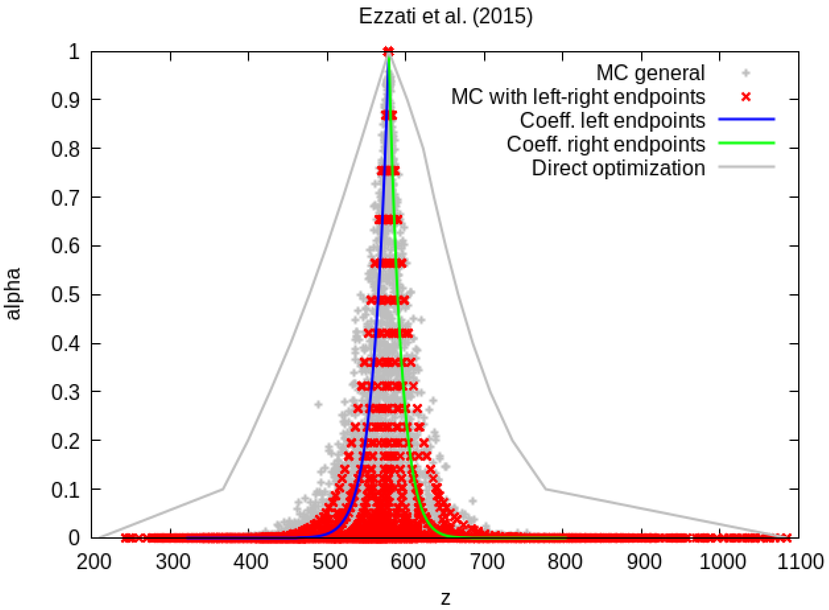
Figure 2 presents the results obtained using the “product” operator to model the conjunction. On the abscissa, the optimal objective values z are represented, while the ordinate is devoted to the α -levels. The general MC simulation algorithm was run 100 times for each k = 1 , 51 ¯ with r 0 , 1 . On the other side, the improved MC algorithm with left-right endpoints was run 10 times for each k = 1 , 51 ¯ with r 0 , 1 . Note that the improved MC algorithm was able to cover the same area with 10 times fewer random generations.
There are several conclusions that can be drawn from this representation:
  • The empiric solution provided by the general MC algorithm (in gray) better covers the exact fuzzy set representing the optimal solution when compared to the left–right-endpoint-based MC algorithm (in red);
  • The empiric fuzzy set solution has a quite large support, but the level set corresponding to α = 0.1 is already 47 % of the level set of α = 0 , and is thus considerably narrower;
  • Even though the FF-LP problem has only non-negative coefficients, no relevant solutions can be obtained either by setting all coefficients to the left endpoints of their α -cuts (in blue) or on their right endpoints (in green), since such derived solutions are too far from the exact ones derived by direct optimization (in gray).

4.2. Second Numerical Example

We proceed with solving the FF-LP problem with trapezoidal fuzzy numbers as coefficients used by Wang and Peng in [4]. We solve
min c ˜ T x ˜ , subject   to a ˜ x ˜ b ˜ , x ˜ 0 ,
where the fuzzy coefficients are TrFNs described by
a ˜ = 19 , 21 , 25 , 26 2 , 4 , 8 , 10 9 , 12 , 16 , 19 6 , 7 , 9 , 12 , b ˜ = 600 , 1000 , 1200 , 1700 500 , 700 , 1100 , 1300 ,
c ˜ T = 4 , 8 , 9 , 12 2 , 3 , 4 , 6 .
The graphical representation of our results are shown in Figure 3. On the abscissa the optimal objective values z are represented, while the ordinate is devoted to the α -levels.
There are important observations that one can derive from this example:
  • The left–right-endpoint-based MC algorithm- and the general MC algorithm-derived solutions (in red and gray, respectively) have a very similar accuracy; thus, the former algorithm performs better due to its higher running speed;
  • The empirical solution very well covers the exact fuzzy set solution (either in red or gray); thus, the proposed methodology can provide good approximate solutions when the exact ones are hard to obtain;
  • The α -cut interval is reduced to 55 % after a small increase in α from 0 to 0.1 ;
  • As in the previous example, the solutions derived by setting all coefficients to the same side of their α -cuts (left in blue or right in green) are not relevant to the decision maker.

5. Discussion

Any good approach to solving large-scale problems must aim to find a balance between the exactness of the derived solution and the simplicity of the solution algorithm. The main advantage of our approach to solving FF-LP problems is in deriving fuzzy set optimal solutions that are more relevant to the decision maker.
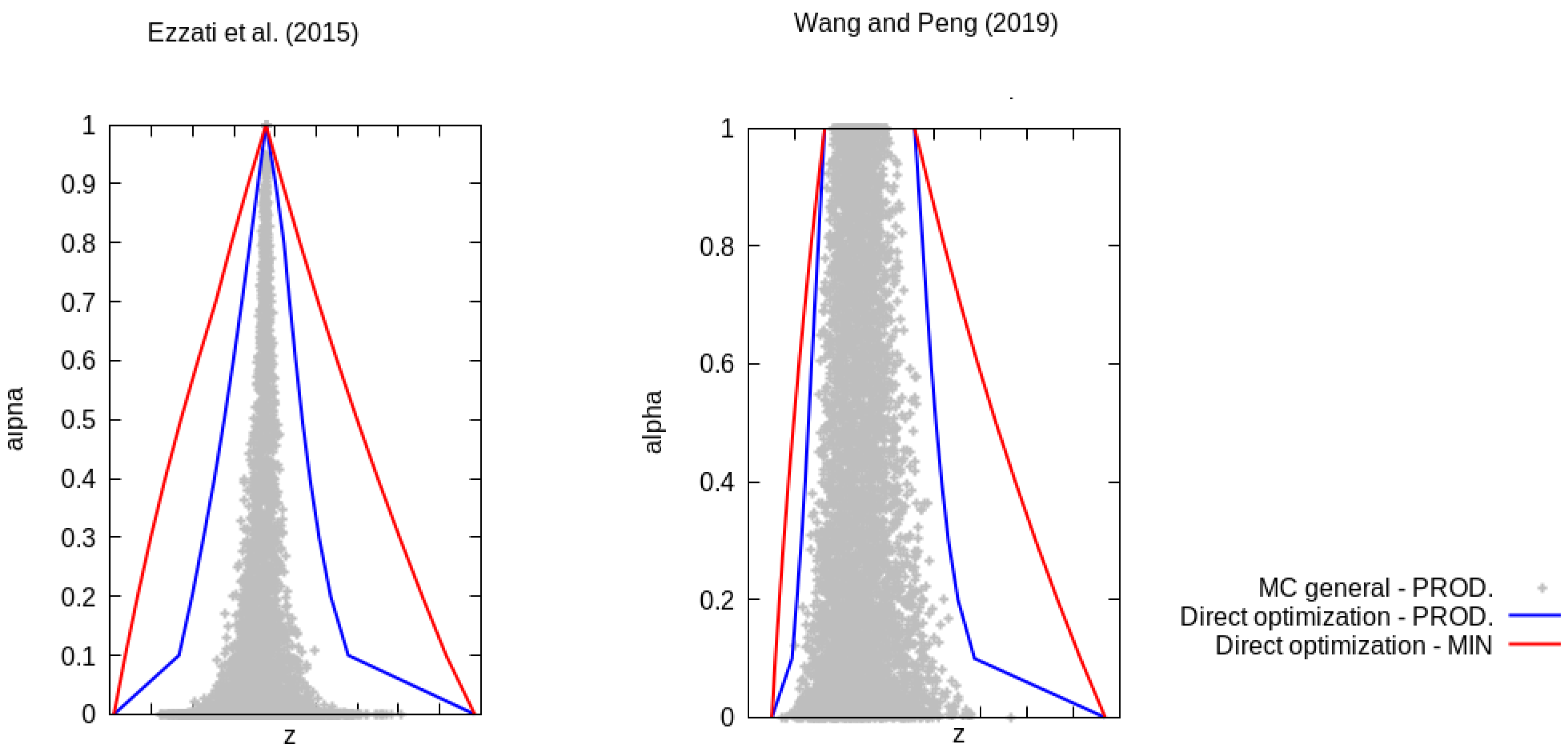
Using the “product” operator instead of the “min” operator to handle the conjunction of fuzzy sets reduces the width of the shapes of the derived results. In fact, the derived solutions have the same support, but when α increases, the α -cut intervals become thinner faster in the first case. An illustration of this fact can be seen in Figure 4. Again, on the abscissa, the optimal objective values z are represented, and on the ordinate, the α -levels are reported.
For both examples recalled from Ezzati et al. [5] and Wang and Peng [4], the solutions derived using the “min” operator are shown in red, while those obtained by using the “product” operator are shown in blue. Numerical values that correspond to several α -cut intervals are reported in Table 2.
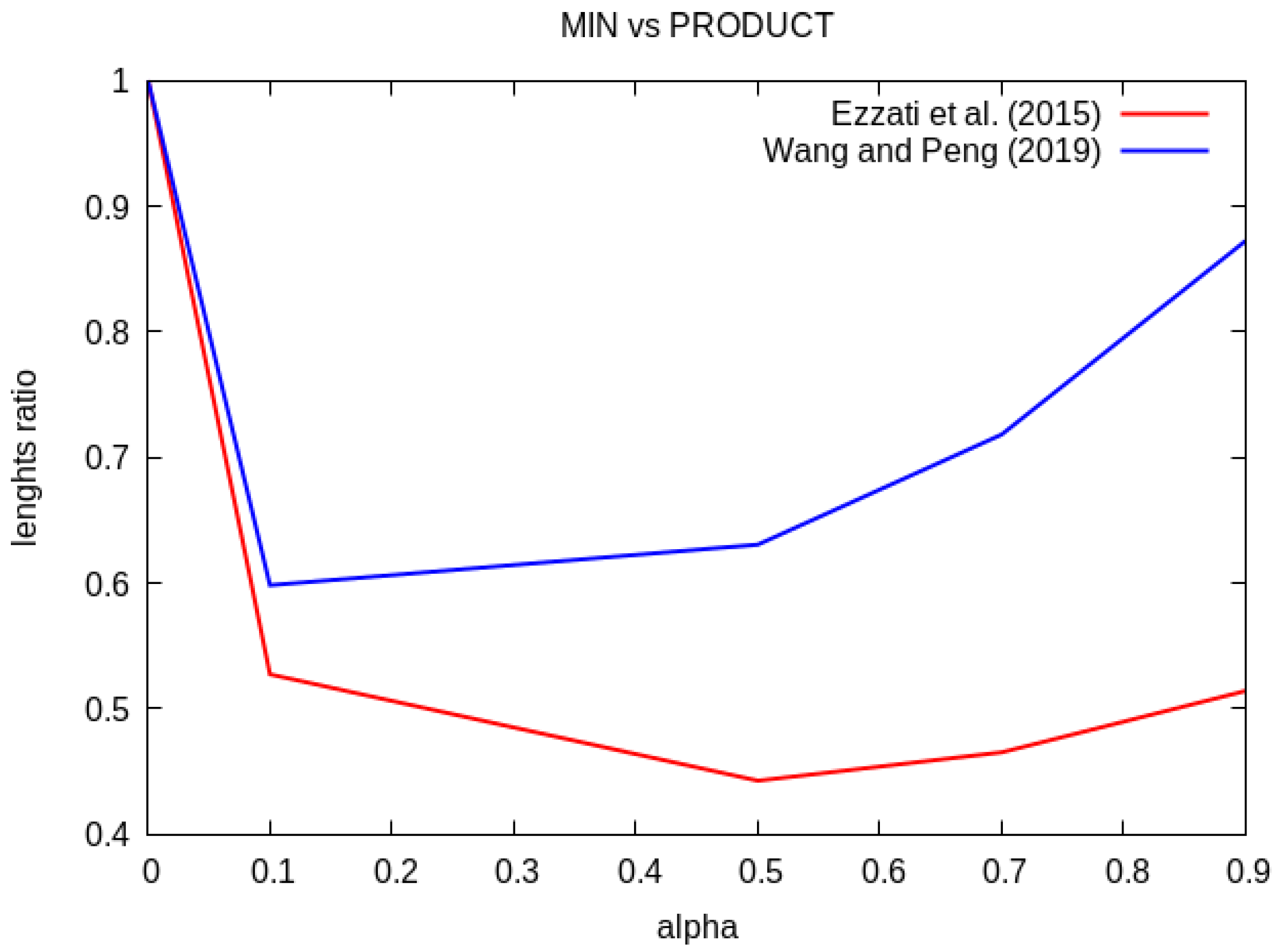
The last column of Table 2 provides the ratio between the lengths of the α -cut intervals of the solutions obtained with the “product” and “min” operators, respectively. For both examples, the ratio has an ample decrease from 1 to 0.53 and 0.60 , respectively, when α increases from 0 to 0.1 (see Figure 5).
On the other hand, for larger values of α , all ratios stay below 0.53 in the first case, but smoothly increase to 0.83 in the second case. These different behaviors are because of different extents of shape symmetry. The TFN representing the optimal solution in the first case is almost symmetric, while the TrFN in the second case is almost vertical on the left side and quite oblique on the right side.
In what follows, we compare the accuracy of the empirical results obtained for the examples recalled from Ezzati et al. [5] and Wang and Peng [4], respectively. With the same number of random generations for each coefficient, the results obtained for the second example are much more accurate (see the gaps between the empiric solutions and the corresponding membership functions derived by direct optimization). The difference in quality is due to the number of coefficients: 14 in the first example and only 8 in the second one. Providing a wider study on how the quality of the empiric results varies with respect to the problem size is not within the scope of this paper, but it may be of interest when applying the approach to solve real-life problems.
Any statistic validation related to the accuracy of the empiric solution in approximating the exact shapes of the fuzzy set solutions is inconceivable, since any statistically relevant analysis demands solving large-scale problems, and the first variant of the proposed approach can hardly be applied to such problems.

6. Conclusions

In this paper, we discussed several solution approaches to FF-LP problems. We emphasized once again the importance of using the EP to unify the fuzzy arithmetic and optimization in a single step and formulated a new procedure to derive empiric optimal solutions to FF-LP problems. We researched the effects of using another aggregating operator instead of the “min” operator for the conjunction of fuzzy sets within fuzzy optimization. The proposed solutions based on the “product” operator are fuzzy sets with narrower shapes; thus, our approach is able to provide more relevant information about the optimal solutions of the modeled system under uncertainty. The solutions derived by our approach are based on the EP and are easier to use in a decision-making process than others from the recent literature.
The main limitation of the proposed approach is that the models able to derive the exact shapes of the fuzzy set optimal values become awkward when the number of the coefficients that define the fuzzy optimization problem increases. Employing heuristics to solve the crisp non-linear optimization problems may simplify the procedure and assure better results. Providing only empiric solutions, the second variant of our approach is less accurate, but it can additionally be used to verify whether (or in what amount) other approaches derive fuzzy solutions in accordance with the extension principle or not.
In our future research, we will address a wider class of mathematical programming problems. We will also choose other operators of generalized products, aiming to provide improved solutions to various fuzzy optimization problems, i.e., more realistic and more concise solutions, to involve in decision making. We will also take into consideration and research the potential formulas that can be derived analytically, using the descriptions provided in [34] for product t norms.

Author Contributions

Conceptualization and methodology, B.S.; writing—original draft and visualization, B.S.; writing—review and editing and validation, S.N. All authors have read and agreed to the published version of the manuscript.

Funding

This work was partly supported by the Serbian Ministry of Education, Science and Technological Development through the Mathematical Institute of the Serbian Academy of Sciences and Arts.

Data Availability Statement

Data are contained within the article.

Conflicts of Interest

The authors declare no conflict of interest.

Abbreviations

The following abbreviations are used in this manuscript:
LPLinear programming
FFFull fuzzy
FNFuzzy number
TFNTriangular fuzzy number
TrFNTrapezoidal fuzzy number
EPExtension principle
MCMonte Carlo
DEAData Enveloped Analysis

References

  1. Lin, Z.; Lin, J.; Xu, Z.; Zhou, Y. Multi-Attribute Decision-Making with Independent Trapezoidal Intuitionistic Fuzzy Information Based on Risk Orientation and Similarity Measure. Int. J. Inf. Technol. Decis. Mak. 2023, 1–41. [Google Scholar] [CrossRef]
  2. Guerra, M.L.; Magni, C.A.; Stefanini, L. Value Creation and Investment Projects: An Application of Fuzzy Sensitivity Analysis to Project Financing Transactions. Int. J. Inf. Technol. Decis. Mak. 2022, 21, 1683–1714. [Google Scholar] [CrossRef]
  3. Stanojević, B.; Stanojević, M.; Nădăban, S. Reinstatement of the Extension Principle in Approaching Mathematical Programming with Fuzzy Numbers. Mathematics 2021, 9, 1272. [Google Scholar] [CrossRef]
  4. Wang, G.; Peng, J. Fuzzy Optimal Solution of Fuzzy Number Linear Programming Problems. Int. J. Fuzzy Syst. 2019, 21, 865–881. [Google Scholar] [CrossRef]
  5. Ezzati, R.; Khorram, V.; Enayati, R. A new algorithm to solve fully fuzzy linear programming problems using the MOLP problem. Appl. Math. Model. 2015, 39, 3183–3193. [Google Scholar] [CrossRef]
  6. Stanojević, B.; Stanojević, M. Empirical versus analytical solutions to full fuzzy linear programming. In Intelligent Methods for Computing, Communications and Control—ICCC2020; Dzitac, I., Dzitac, S., Filip, F., Kacprzyk, J., Manolescu, M., Oros, H., Eds.; Advances in Intelligent Systems and Computing; Springer: Cham, Switzerland, 2020; Volume 1243. [Google Scholar] [CrossRef]
  7. Stanojević, B.; Stanojević, M. Analytic description of fuzzy set solutions to fuzzy “LP” problems. In Proceedings of the SYM-OP-IS 2022, Vrnjačka Banja, Serbia, 19–22 September 2022; pp. 425–429. [Google Scholar]
  8. Anukokila, P.; Radhakrishnan, B. Goal programming approach to fully fuzzy fractional transportation problem. J. Taibah Univ. Sci. 2019, 13, 864–874. [Google Scholar] [CrossRef]
  9. Ebrahimnejad, A.; Verdegay, J. A new approach for solving fully intuitionistic fuzzy transportation problems. Fuzzy Optim. Decis. Mak. 2018, 17, 447–474. [Google Scholar] [CrossRef]
  10. Liu, S.T.; Kao, C. Solving fuzzy transportation problems based on extension principle. Eur. J. Oper. Res. 2004, 153, 661–674. [Google Scholar] [CrossRef]
  11. Liu, S.T. Fractional transportation problem with fuzzy parameters. Soft Comput. 2015, 20, 3629–3636. [Google Scholar] [CrossRef]
  12. Mahajan, S.; Gupta, S. On fully intuitionistic fuzzy multiobjective transportation problems using different membership functions. Ann. Oper. Res. 2019, 296, 211–241. [Google Scholar] [CrossRef]
  13. Mahmoodirad, A.; Allahviranloo, T.; Niroomand, S. A new effective solution method for fully intuitionistic fuzzy transportation problem. Soft Comput. 2019, 23, 4521–4530. [Google Scholar] [CrossRef]
  14. Mishra, A.; Kumar, A. JMD method for transforming an unbalanced fully intuitionistic fuzzy transportation problem into a balanced fully intuitionistic fuzzy transportation problem. Soft Comput. 2020. [Google Scholar] [CrossRef]
  15. Stanojević, B.; Stanojević, M. Solution value envelope to full fuzzy transportation problems. In Proceedings of the SymOrg 2020, Faculty of Organizational Sciences, Belgrade, Serbia, 7–9 September 2020; pp. 319–326. [Google Scholar]
  16. Stanojević, B.; Stanojević, M. Approximate membership function shapes of solutions to intuitionistic fuzzy transportation problems. Int. J. Comput. Commun. Control 2021, 16, 4057. [Google Scholar] [CrossRef]
  17. Kao, C.; Liu, S.T. Fuzzy efficiency measures in data envelopment analysis. Fuzzy Sets Syst. 2000, 113, 427–437. [Google Scholar] [CrossRef]
  18. Kao, C.; Liu, S.T. Efficiencies of two-stage systems with fuzzy data. Fuzzy Sets Syst. 2011, 176, 20–35. [Google Scholar] [CrossRef]
  19. Soltanzadeh, E.; Omrani, H. Dynamic network data envelopment analysis model with fuzzy inputs and outputs: An application for Iranian Airlines. Appl. Soft Comput. 2018, 63, 268–288. [Google Scholar] [CrossRef]
  20. Zhou, W.; Xu, Z. An Overview of the Fuzzy Data Envelopment Analysis Research and Its Successful Applications. Int. J. Fuzzy Syst. 2020, 22, 1037–1055. [Google Scholar] [CrossRef]
  21. Sotoudeh-Anvari, A. A critical review on theoretical drawbacks and mathematical incorrect assumptions in fuzzy OR methods: Review from 2010 to 2020. Appl. Soft Comput. 2020, 93, 106354. [Google Scholar] [CrossRef]
  22. Ghanbari, R.; Ghorbani-Moghadam, K.; De Baets, B. Fuzzy linear programming problems: Models and solutions. Soft Comput. 2019, 24, 1433–7479. [Google Scholar] [CrossRef]
  23. Zadeh, L. Fuzzy sets. Inf. Control 1965, 8, 338–353. [Google Scholar] [CrossRef]
  24. Shi, Y. My Early Researches on Fuzzy Set and Fuzzy Logic. Int. J. Comput. Commun. Control 2021, 16, 4090. [Google Scholar] [CrossRef]
  25. Dubois, D.; Prade, H. Fuzzy sets and systems: Theory and applications. In Mathematics in Science and Engineering; Universite Paul Sabatier: Toulouse, France, 1980. [Google Scholar]
  26. Zadeh, L. The concept of a linguistic variable and its application to approximate reasoning I. Inf. Sci. 1975, 8, 199–249. [Google Scholar] [CrossRef]
  27. Ross, T. Fuzzy Arithmetic and the Extension Principle. In Fuzzy Logic with Engineering Applications; John Wiley & Sons, Ltd.: Hoboken, NJ, USA, 2010; Chapter 12; pp. 408–436. [Google Scholar] [CrossRef]
  28. Zimmermann, H.J. Fuzzy programming and linear programming with several objective functions. Fuzzy Sets Syst. 1978, 1, 45–55. [Google Scholar] [CrossRef]
  29. Bellman, R.E.; Zadeh, L.A. Decision-Making in a Fuzzy Environment. Manag. Sci. 1970, 17, B141–B164. [Google Scholar] [CrossRef]
  30. Radojević, D. Interpolative Realization of Boolean Algebra as a Consistent Frame for Gradation and/or Fuzziness. In Forging New Frontiers: Fuzzy Pioneers II; Springer: Berlin/Heidelberg, Germany, 2008; pp. 295–317. [Google Scholar] [CrossRef]
  31. Milošević, P.; Petrović, B.; Radojević, D.; Kovačević, D. A software tool for uncertainty modeling using Interpolative Boolean algebra. Knowl.-Based Syst. 2014, 62, 1–10. [Google Scholar] [CrossRef]
  32. Milošević, P.; Nešić, I.; Poledica, A.; Radojević, D.; Petrović, B. Logic-based aggregation methods for ranking student applicants. Yugosl. J. Oper. Res. 2017, 27, 463–479. [Google Scholar] [CrossRef]
  33. Brunelli, M.; Mezei, J. How different are ranking methods for fuzzy numbers? A numerical study. Int. J. Approx. Reason. 2013, 54, 627–639. [Google Scholar] [CrossRef]
  34. Soylu, G.; Aslan, M.E. Fuzzy arithmetic with product t-norm. Iran. J. Fuzzy Syst. 2021, 18, 185–197. [Google Scholar] [CrossRef]
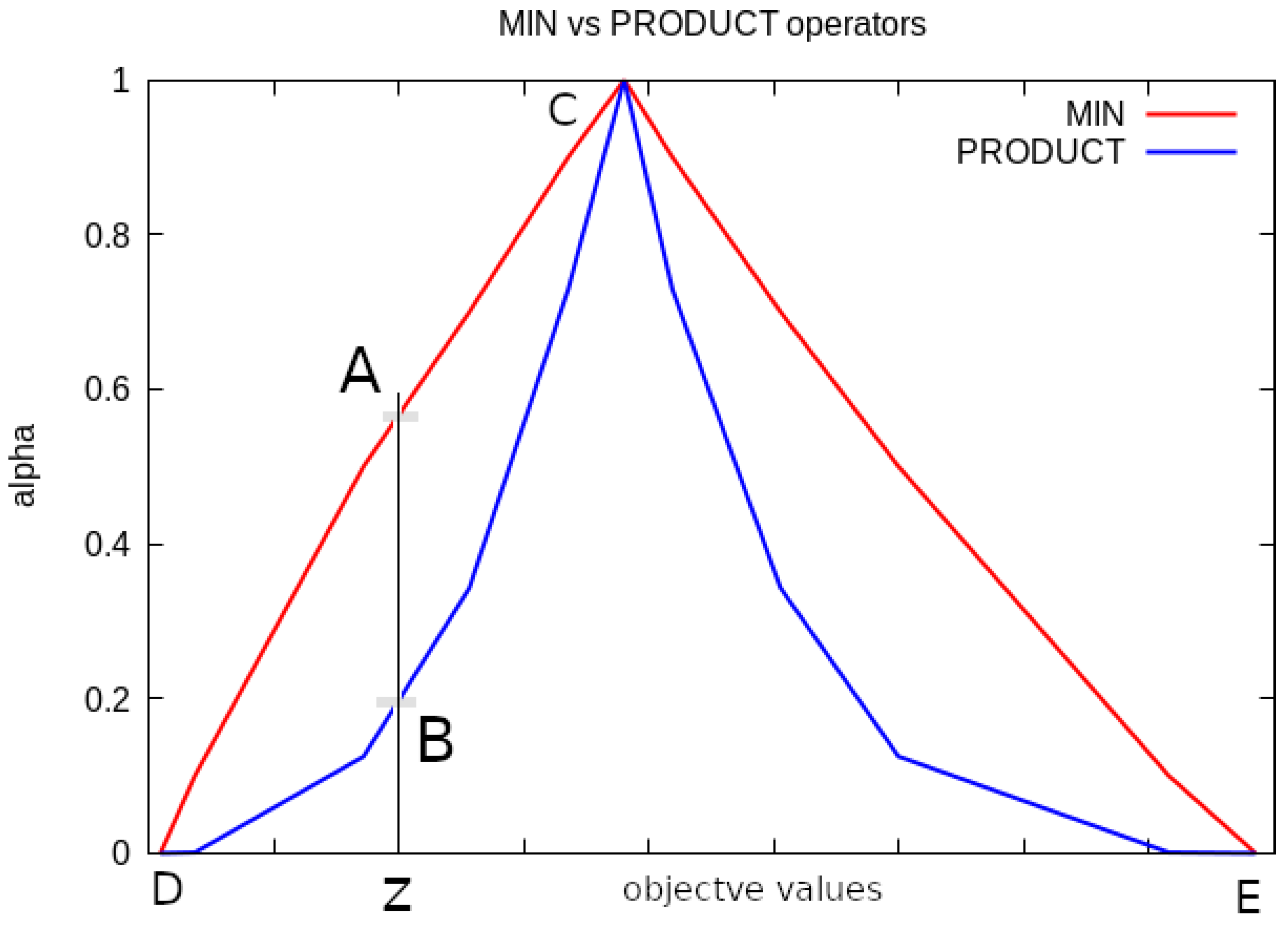
Figure 1. The illustration of the results formalized in Proposition 2.
Mathematics 11 04864 g001
Figure 2. Graphic representation of the empiric objective values obtained to Problem (19) by running the general Monte Carlo simulation algorithm and the Monte Carlo simulation algorithm based on the left and right endpoints of the α -cut intervals [5].
Mathematics 11 04864 g002
Figure 3. Graphic representation of the empirical objective values obtained to Problem (27) by running the general Monte Carlo simulation algorithm and the Monte Carlo simulation algorithm based on the left and right endpoints of the α -cut intervals [4].
Mathematics 11 04864 g003
Figure 4. Graphical comparison of the results obtained by using min and product operators for solving Problems (19) and (27) [4,5].
Mathematics 11 04864 g004
Figure 5. Length ratio variation with respect to the α -level [4,5].
Mathematics 11 04864 g005
Table 1. Brief literature review on full fuzzy mathematical programming problems.
AuthorsYearRef.ProblemFull Compliance to the EP
Stanojević et al.2021[3]review fuzzy LP and LFPN/A
Wang et al.2019[4]FF-LPyes
Ezzati et al.2015[5]FF-LPno
Anukokila et al.2019[8]transportation FF-LFPno
Ebrahimnejad et al.2018[9]transportation FF-LFPno
Liu et al.2004[10]transportation FF-LFPyes
Kao et al.2000[17]fuzzy DEAyes
Kao et al.2011[18]fuzzy DEAyes
Soltanzadeh et al.2018[19]fuzzy DEAno
Ghanbari et al.2019[22]review fuzzy LPN/A
Table 2. Numerical comparison of the results obtained by using min versus product operators in solving Problems (19) and (27).
Problem α min α -Cuts and LengthsProduct α -Cuts and LengthsLengths Ratio 1
(19) 0.9 535.17 , 618.46 83.29 558.77 , 601.61 42.84 0.51
0.7 456.13 , 704.91 248.78 519.78 , 635.58 115.80 0.47
0.5 371.47 , 799.38 427.92 476.90 , 666.42 189.53 0.44
0.1 236.51 , 1015.57 779.06 366.90 , 777.86 410.95 0.53
0.0 209.04 , 1085.0 875.96 209.04 , 1085.0 875.96 1
(27) 0.9 296.6 , 778 481.4 312.78 , 732.73 419.94 0.87
0.7 241.4 , 914 672.6 284.74 , 767.88 483.14 0.72
0.5 192.7 , 1066 873.3 256.70 , 807.45 550.75 0.63
0.1 114.2 , 1431 1316.8 185.86 , 973.82 787.96 0.60
0.0 98.36 , 1537.5 1439.14 98.36 , 1537.5 1439.14 1
1 The ratio between the lengths of the product and min α -cuts.
Disclaimer/Publisher’s Note: The statements, opinions and data contained in all publications are solely those of the individual author(s) and contributor(s) and not of MDPI and/or the editor(s). MDPI and/or the editor(s) disclaim responsibility for any injury to people or property resulting from any ideas, methods, instructions or products referred to in the content.