Deciphering the Innovation Subsidy Puzzle: Government Choices amid Supply Chain Encroachment

Abstract

Although the impact of government subsidies on private innovation has been widely recognized and researched in numerous studies, few have considered the increasingly prevalent phenomenon of supply chain encroachment in their analysis. This paper explores this phenomenon through a game-theoretic model that takes into account a government entity, a supplier, and a manufacturer. The primary aim is to understand how the government can make optimal subsidy decisions when the supplier moves into the supply chain. Several interesting conclusions have been drawn: (1) under governmental innovation subsidies, the supplier will raise the price of the new technology to obtain more potential revenue, which is termed the inverse wholesale price effect; (2) different kinds of innovation subsidies are shown to have varied effects on R&D, production, and consumption behavior; and (3) different subsidy strategies are made compatible with the characteristics of innovative activities to maximize social welfare as much as possible. These findings shed light on inconsistent results surrounding the impacts of government subsidies on private innovations in the existing literature, providing municipalities with helpful guidance when encouraging private innovation initiatives amid supply chain encroachment.

1. Introduction

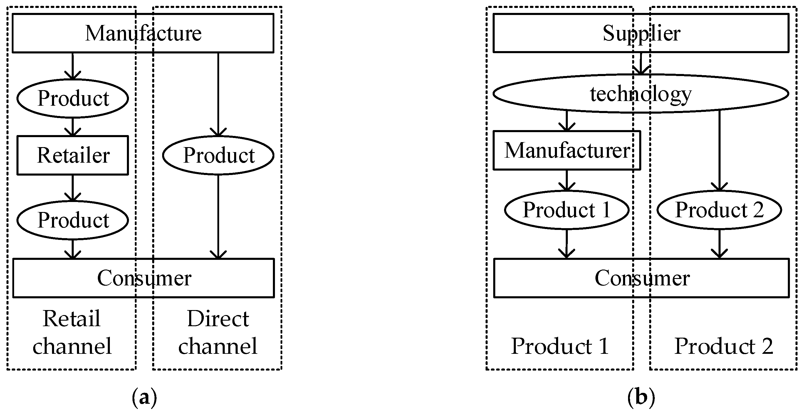
Traditional supply chain encroachment typically manifests when upstream manufacturers invest in direct-to-consumer channels, such as online stores, thus entering into competition with their own retailers in the consumer market [1]. Contrastingly, an emerging and less-explored form of encroachment involves upstream suppliers who, while providing technological support to downstream manufacturers, concurrently engage in the production and sale of competitive end products. This scenario creates a market dynamic where multiple product types coexist within the supply chain, leading to direct competition between upstream suppliers and downstream manufacturers. This complex interaction is illustrated in Figure 1, which depicts the layered relationships and competitive landscape within this evolved supply chain structure. For example, Microsoft, a provider of computer operating systems, routinely designs technology updates that are sold to computer hardware manufacturers like Dell and Lenovo. When touch control technology was a novelty, Microsoft created its own laptop called the Surface for Windows 8 in June 2012; this provided competition for PC hardware manufacturers [2]. In 2016, Google—maker of the Android mobile operating system—declared they would be releasing the Google Pixel phone to consumers [3]. Samsung Electronics, the owner of OLED screen technology, supplies these screens to Apple while competing with Apple by using them in its own smartphones [4]. BYD, China’s largest new-energy vehicle maker, also supplies batteries to the Great Wall Motor Group (GWM).

This kind of encroachment not only affects the decision-making process of each stakeholder in the supply chain (such as suppliers, manufacturers, and consumers) but also poses a dilemma for government initiatives aimed at promoting innovation through subsidies. When the technological supplier (he) encroaches the product market of the downstream manufacturer (she), his revenue is derived from two main sources: profits from selling own-brand products and income generated by providing technical support to the downstream manufacturer. If the government subsidizes the price of the manufacturer’s products, typically, the demand of the manufacturer’s products increases. Consequently, the frequency of the manufacturer purchasing technical support from the technological supplier rises, and as a result, the supplier’s revenue generated from providing technical support increases. However, government subsidies on the price of the manufacturer’s products often lead to a decrease in the demand of the supplier’s own-brand products, consequently reducing the supplier’s profit from the sales of these products. It is evident that when the government subsidizes the price of the manufacturer’s products, the impact on the expected income of the supplier is uncertain. Therefore, predicting the influence of subsidies on the supplier’s innovation decisions and on social welfare is challenging. If the government subsidizes the price of the supplier’s products, typically, the demand of the supplier’s own-brand products increases, but the demand of the manufacturer’s products decreases. This results in an increase in the expected income from the sale of own-brand products by the supplier, but the decrease in the demand of the manufacturer’s products also leads to a decline in the revenue for technical support from the supplier. The impact of subsidies on the expected income of the supplier is also unclear. Of course, the government can directly subsidize the innovation costs of the supplier; however, it is not yet clear whether cost subsidies have an absolute advantage over price subsidies in enhancing social welfare and promoting technological innovation. It is evident that for the government, devising a precise and efficient subsidy policy faces significant challenges when confronted with the increasingly prevalent market structure changes brought about by technological suppliers encroaching the supply chain.

However, existing research primarily focuses on analyzing the impact of supply chain encroachment under the traditional model on the decision making of suppliers and manufacturers. They concentrate on aspects such as the choice of sales channels [5], the analysis of market conditions for manufacturer encroachment [6], and the positioning analysis of products encroaching the market [6]. There is a dearth of research that adopts a governmental perspective to analyze the optimal subsidy strategy when technological suppliers encroach the product market of manufacturers. In practice, in the absence of reference and guidance, governments often provide subsidies to all enterprises that meet specific criteria at each stage of the supply chain. For instance, the Public Notice on Preliminary Review issued by the Chinese Ministry of Technology provides insights into the financial support received by GWM and BYD in 2021, with GWM receiving RMB 1817.49 million and BYD receiving RMB 5229.89 million [7]. Additionally, BYD’s 2021 financial report reveals that they were granted R&D subsidies of RMB 5833 thousand specifically for lithium-ion batteries. However, such an approach imposes significant fiscal pressure that cannot be ignored. Therefore, it is essential to assist governments in determining the recipients and devising effective mechanisms for subsidy allocation.

This paper is poised to solve the conundrum that government policy-makers face: how to effectively provide subsidies when a supplier is encroaching upon the market of a manufacturer. Technological suppliers are motivated to engage in higher levels of technological innovation only when the government’s subsidy policy effectively enhances their expected income. As for consumers, their purchasing behavior is influenced only when government subsidies have the potential to alter consumer surplus [8]. From the government’s perspective, a subsidy policy is deemed effective only when the combined improvement of the expected income of suppliers and manufacturers, along with consumer surplus (i.e., social welfare), is achieved [9,10]. Therefore, this study will focus on three overarching research questions: (1) How do different strategies for providing subsidies influence the optimal decisions and returns of suppliers and manufacturers? (2) How do different types of subsidies affect purchasing behavior among consumers? (3) Under what conditions are certain subsidy policies more applicable than others?

This paper builds four game-theoretic models and investigates the effect of four subsidy policies offered by the government on the supplier’s innovation activities and competitive relationships between the supplier and the manufacturer. The models are based on a scenario consisting of a supplier, a manufacturer, and the government. In this situation, the supplier implements technological innovation and produces their private brand product which encroaches upon the manufacturer’s market. The manufacturer buys this new technology from the supplier to incorporate it into their own products for sale in the market. While promoting social welfare, the government subsidizes innovative activities implemented by suppliers. Considering the diversification of government innovation subsidies and the maneuverability of model building, this paper abstracts government subsidies into three situations according to the objects of subsidies [10,11]. These models involve Bertrand competition wherein each participant decides their own product’s price [12], as well as a Stackelberg game model in which the government acts as a leader while suppliers and manufacturers act as followers under conditions of subsidies [13].

This paper is the first to model government innovation subsidy strategies in a setting of supply chain encroachment. We solve our model and analyze the optimal decision-making, expected revenue, and social welfare of firms under various subsidy policies; in doing so, we determine the applicable conditions of each policy. Our main results are as follows: (1) With reference to previous research conclusions and our own model analysis, we observe that when the government subsidizes a supplier’s product, they will raise selling prices to gain more expected revenue—what we call an “inverse wholesale price effect”. (2) Both the supplier and manufacturer experience increased expected revenue when governments provide subsidies for either the manufacturer’s product or the innovation cost of the supplier. (3) When governments subsidize the price of a manufacturer’s product, its consumer surplus change depends on the market profitability coefficient of the new technology; on the other hand, when subsidies are provided for a supplier’s product, changes depend on the amount of government subsidy. (4) Each subsidy has specific circumstances under which it can be effectively applied; although cost subsidies can be used in many cases, their effects on social welfare are limited. Comparatively, price subsidies have fewer applications but a higher payoff in terms of social welfare gains.

The remainder of this paper is organized as follows. Section 2 presents a literature review. Section 3 outlines the model setting. Section 4 establishes models of government’s different subsidy strategies in response to supply chain encroachment. The comparative analysis of the government’s optimal innovation subsidy strategy decision is covered in Section 5. Lastly, Section 6 concludes this paper, and all proofs are presented in the Appendix B.

2. Literature Review

Two areas of research are related to this study: supply chain encroachment and government subsidies. Studies examining supply chain encroachment hold relevance to the supply chain structure outlined in this paper. Government subsidies are central to this study’s discussion. We will then assess and contextualize comparably aligned studies within each respective area, as well as highlight the distinctions between this study and the current literature.

The first area of research pertains to supply chain encroachment. The scenarios analyzed in existing studies on supply chain encroachment primarily focus on competition issues among different sales channels. Specifically, supply chain encroachment often refers to a manufacturer establishing a direct sales channel (particularly through an online platform) in addition to the existing retail channel to directly sell their products to consumers. Prior research on supply chain encroachment has concentrated on examining influencing variables such as information sharing [14,15,16], technical breakthroughs [1,17], promotional collaboration [18], and differences in channel structure [19,20]. The existing literature exhibits at least two commonalities. Firstly, concerning the structure of the studied supply chains, these analyses typically involve the same product being sold through different channels. However, as market competition relationships become increasingly intricate, the issue of supply chain encroachment extends beyond mere competition among different channels for the same product. Larger retailers, platforms, or suppliers also produce substitute products and distribute them across various channels [6,21,22]. Presently, there are few studies that specifically analyze the issue of supply chain encroachment through competitive products, although they do exist [23]. Hence, it is also challenging to find reference points within the literature for the specific encroachment scenario that this paper aims to explore, which involves technology suppliers producing alternative products to encroach upon downstream manufacturers’ markets. Furthermore, the existing literature predominantly focuses on the analysis within the internal dynamics of the supply chain. Whether examining the optimal timing for invaders’ incursion or assessing the impact of intrusion on the expected benefits of different entities within the supply chain [24], these analyses concentrate on how the act of intrusion influences the decision-making behaviors of various entities within the supply chain. However, supply chain intrusion not only affects different entities within the supply chain but also influences the decision making of stakeholders outside the supply chain, such as governments. It is widely acknowledged that government subsidies encouraging social innovation are influenced by market structures [25,26]. When encroachment occur within the supply chain, not only does the structure of the supply chain alter, but the variety of products within the supply chain also changes, leading to significant shifts in market structure. These changes inevitably impact the optimal choice of government subsidy strategies [10]. Nevertheless, there is limited analysis in the existing literature regarding the influence of supply chain encroachment on government subsidy policies, creating an opportunity for exploration within this research.

A secondary stream of research concerns government innovation subsidies, wherein governments offer financial support to stimulate private innovative activities [27]. Over the past two decades, an enduring academic discourse has surrounded the impact of government innovation subsidies on private innovation [28]. Most of these studies employ an empirical research paradigm, utilizing panel data to scrutinize the effect of government subsidies on firms’ innovation endeavors [29]. While some studies suggest a positive influence of government subsidies [30,31], others highlight their potential to crowd out private investment [32,33]. However, other studies find no explicit relationship between government subsidies and private innovation [34,35]. The inconsistencies observed in these studies might stem from the limitations of panel data analysis in thoroughly elucidating the decision-making logic and game mechanisms at the micro-level of various actors. Presently, there are also works utilizing behavioral decision models to conduct relevant research. These studies often emphasize the exploration of the diverse impact of various government subsidy policies on the optimal decisions of different actors within the supply chain (such as R&D strategies, competitive strategies, collaborative strategies, etc.) and their expected revenues [36,37]. Various studies typically introduce distinct factors into their analyses (such as consumer preferences, product eco-friendliness, etc.) [38,39]. However, these works often treat government subsidies as exogenous variables and analyze their impact on firms’ decision making from an enterprise perspective. There is a paucity of research adopting the government’s standpoint to analyze the optimal selection of innovation subsidy strategies within the context of supply chain encroachment.

Our study builds upon the existing literature but innovatively approaches the topic by discussing government subsidy strategies in the context of supply chain encroachment (unique to this study). To more accurately analyze the optimal government innovation subsidy strategy, we improved the model for supply chain encroachment based on vertical differentiation theory to facilitate the calculation of government expected returns. Furthermore, in this paper, we have integrated elements of innovation, such as the market profitability of technological innovation achievements, which play a pivotal role in government subsidization decisions. We have employed a variety of factors to model these aspects. While conventional research often focuses on consumer-specific factors when constructing models to analyze optimal government subsidy strategies or businesses’ optimal research and development decisions, such as consumers’ green preferences and environmental awareness, this paper places a greater emphasis on the characteristics of technological innovation activities, which significantly aids in the analysis of optimal government subsidy strategies. Lastly, this article combines the characteristics of innovation projects and the level of market competitiveness to analyze the implementation conditions of different subsidy policies. The existing literature predominantly examines the impact of different subsidy policies on expected business returns and product consumer surplus, with minimal attention to the analysis of the conditions under which these subsidy policies are applicable. However, choosing the appropriate subsidy conditions is not only a key concern for the government but also a prerequisite for subsequent studies on subsidy effectiveness. Therefore, this paper places a significant emphasis on analyzing the applicability conditions of different subsidy policies.

3. The Model Description and Assumptions

We consider the interplay between a supplier ($S$), a manufacturer ($M$), and a government ($G$). The manufacturer buys technology from the supplier who is engaged in innovating new technology to improve consumer evaluations of the manufacturer’s products. While this occurs, the supplier also produces their own product using the same technology. For instance, when computer manufacturers pre-install the Windows operating system on the computers they produce, they incur a pre-installation fee to Microsoft for each unit [40]. Concurrently, Microsoft also manufactures its own personal computers, such as the Surface. 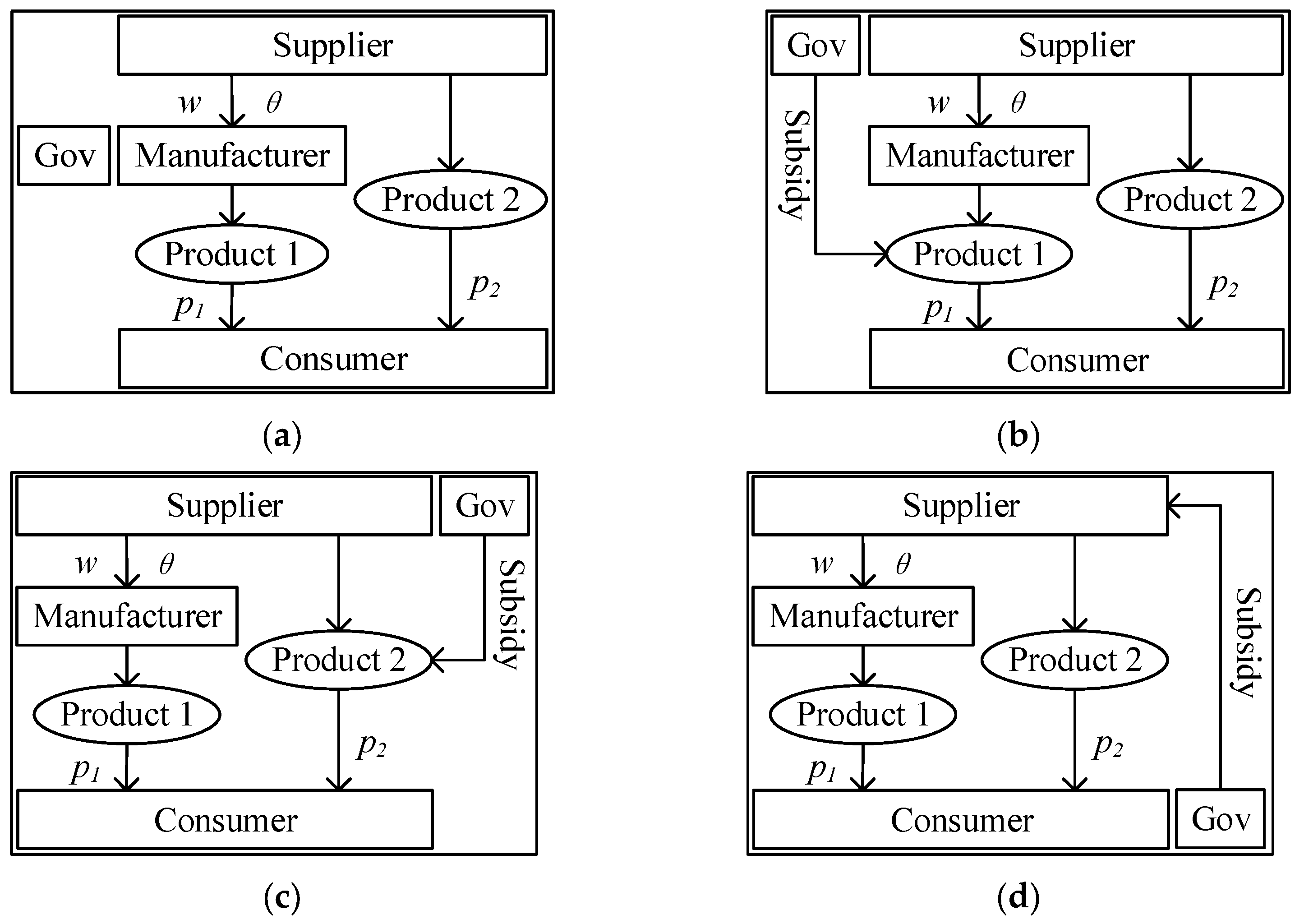To improve social welfare, governments have various incentives to encourage technology innovation, such as grants, tax concessions, or a discount on the price of a product, or provide support for the R&D expenses of enterprises in the form of projects [41]. In order to clarify the influence mechanism of different subsidies on different objects in the supply chain, according to the subject and stages of innovation subsidy effect, this paper abstracts various government subsidy methods into four basic subsidy strategies: firstly, subsidizing according to the price of the manufacturer’s product (strategy $SM$); secondly, subsidizing according to the price of the supplier’s product (strategy $SS$); and thirdly, subsidizing according to the cost of innovation (strategy $SC$). Sometimes, governments refrain from subsidizing innovation activities. For instance, this could occur when the government perceives that the development of a particular technology does not align with the national development strategy or falls outside the areas of primary government focus. Alternatively, it may happen when the government, after considering factors such as the market acceptance of new technologies, technological maturity, and commercialization potential, deems the timing for subsidization as premature. Also, if the market provides adequate returns for a specific technology, effectively incentivizing innovation within enterprises, the government might opt not to provide subsidies. In such cases, this paper categorizes this scenario under strategy NS, denoting the absence of subsidies. Figure 2 illustrates the relationships among these players and contextually describes this study.

The manufacturer sets the selling price $p_1$ for her own product. The supplier determines the level of innovation $\theta$ he wish to pursue, the unit technology selling price $w$, and the selling price $p_2$ for his product. Note that the unit product price is more expensive than the unit technology price, i.e., $p_i>w$, where $i=1, 2$. When $p_i<w$, producing such a product will not yield positive economic returns for the producer. Consequently, production activities will not take place [42]. As Cabral highlighted in his seminal work, the occurrence of either price or quantity competition is contingent upon the specific industry dynamics. Industries where capacity and output can be readily adjusted, such as software, insurance, and banking, tend to align more closely with the Bertrand model in representing market competition [43,44]. In this paper, the primary focus revolves around technological suppliers like Microsoft, Cisco, and Alibaba. For these suppliers, given their capability to easily adjust capacity and output, we adopt the Bertrand setting in our analysis.

To foster innovation, governmental bodies commonly extend financial incentives to bolster corporate endeavors in this realm. These incentives encompass diverse forms, embracing but not being limited to cost subsidies, price subsidies, tax advantages, and talent acquisition incentives, among others [45]. By scrutinizing the pivotal role of subsidies within the supply chain, these incentives bifurcate into two principal categories [13]. First, price subsidies are situated at the demand side (inclusive of subsidies on product prices, exemptions from purchase taxes, etc.). For instance, in support of digital transformation among small and medium enterprises, the Chinese government offers up to a 30% price subsidy to each pilot enterprise leveraging digital public service platforms for digitalization [46]. Second, cost subsidies are positioned at the supply side (encompassing subsidies targeting research and development expenses, talent acquisition outlays, etc.). For example, in 2019, the United Kingdom’s innovation agency, Innovate UK, allocated GBP 20 million in research and development funding to bolster the advancement of advanced low-carbon propulsion in the automotive sector [13].

Following [13,47], if the government institutes a price subsidy, denoted by $\mu$, and consumers purchase an innovative product initially priced at $p_i$, the implementation of the government’s subsidy results in consumers bearing a reduced cost, where the adjusted expense equates to $p_i-\mu$ for that product.

As noted by Takalo, government cost subsidies for private innovation are anticipated to reduce the marginal cost of innovation activities, consequently stimulating firms to invest more in technological innovation [48]. Referring to the existing literature regarding the establishment of government cost subsidies [25,44], this study introduces $\tau$ to symbolize the proportion allocated for cost subsidy. In a scenario where a supplier incurs innovation expenses amounting to $C$, the implementation of government cost subsidies would diminish their essential expenditure to $\left(1-\tau \right)C$, with supplementary costs being subsidized by the government in a magnitude equivalent to $\tau C$.

The game sequence can be depicted as Figure 3. In the first stage, the government decides on subsidy programs that maximize social welfare [49,50]. Given that technological innovation requires much more time than production, we assume that the innovation level is determined before the price of the product is set. Therefore, in the second stage, the supplier decides the level of innovation ($\theta$) and the price of their new technology ($w$). In the third stage, manufacturers and suppliers decide the prices for products 1 and 2 at the same time.

3.1. Demand Functions

This paper adopts the vertical differentiation theory to construct demand functions. This choice is motivated by two primary considerations. Firstly, in contrast to alternative theories like horizontal differentiation theory, which evaluate how varied product attributes impact market equilibrium, the vertical differentiation theory is better poised to analyze the influence of technological innovation on consumer behavior. The vertical differentiation theory excels in examining the impact of alterations in a singular product attribute, such as the security of data, or the compatibility of products, on consumer preferences. Technological innovation frequently concentrates on refining a specific product attribute. Numerous investigations into enterprise R&D decisions also rely on the vertical differentiation theory [51,52]. Additionally, the vertical differentiation theory offers a precise depiction of market competitive dynamics and furnishes an exact resolution for consumer surplus—an integral component of anticipated government revenue. Many extant studies leverage the vertical differentiation theory to scrutinize governmental optimal decision making [38,45].

According to the vertical differentiation theory, we assume that customers are diverse in their evaluations of new technology and each customer’s reservation price $\xi$ is uniformly distributed from 0 to 1, which accounts for individual differences in product valuation [42]. The net utilities of a customer purchasing products 1 and 2 can be, respectively, expressed as follows:

$$\left\{\begin{array}{c}{u}_1=\xi -p_1\\ u_2=s\xi -p_2\end{array}\right.$$

(1)

where $s$ describes the differentiation between products 1 and 2, and $s\in \left(\mathrm{0,1}\right)$. Since the manufacturer’s product is well known by the customers, we assume that the brand value of product 1 is higher than that of product 2. As a result, the consumers’ reservation price of product 1 ($\xi$) is higher than that of product 2 ($s\xi$). Certainly, we can assume that the consumers value the supplier’s product more. However, due to the symmetrical relationship, the research conclusions would not change. Similar to existing research, we assume that $p_i$ has a leading coefficient of 1 [13,41].

Regarding technological innovation, we draw upon Bhaskaran and Krishnan’s simulation methodology for assessing technological innovation uncertainty to construct the research model in this paper. We assume that the target level set by the technological supplier is denoted as $\theta$. According to Bhaskaran and Krishnan, one aspect of innovation uncertainty is translational uncertainty, signifying that while the supplier can establish a target level of innovation, the certainty of achieving that target remains uncertain due to the possibility that the technological environment may not adequately support the development of the relevant technology [53]. For instance, in contexts where large-scale data operations are not feasible, the development of active noise reduction technology poses significant challenges. Denote $\tilde{v}$ as the translational uncertainty; $\tilde{v}$ is uniformly distributed between $\underset{\_}{v}$ and 1. The closer $\underset{\_}{v}$ is to 1 (0), the greater the possibility that the innovation will be a success (failure). $E\left(\tilde{v}\right)=\frac{1+\underset{\_}{v}}{2}=v$. $\underset{\_}{v}\in \left(\mathrm{0,1}\right)$ [53].

Furthermore, technology adoption is also uncertain. Although the aim of technological innovation often lies in enhancing the consumers’ product usage experience, the customers of such products may exhibit diverse behaviors in adopting innovative products, as supported by innovation adoption theories [54]. For instance, the adoption decisions regarding IBS (Industrialized Building System) technology within the construction industry are heavily influenced by a multitude of factors such as economic, social, and political aspects, resulting in significant uncertainty [55]. Following [56], we denote $r$ as the technology adoption. $r\in \left[\mathrm{0,1}\right)$. The closer $r$ is to 1 (0), the more popular (unpopular) the new technology is. $r$ and $\tilde{v}$ are assumed to be independent from each other, thus subsequently leading to a customer’s additional reservation price after innovation being $r\tilde{v}\theta$, while also resulting in an alteration in their net utility when purchasing two products being:

$$\left\{\begin{array}{c}{u}_1=\xi +r\tilde{v}\theta -p_1\\ u_2=s\left(\xi +r\tilde{v}\theta \right)-p_2\end{array}\right.$$

(2)

3.2. Cost of Innovation

Following [53], we postulate that the cost of technological innovation consists of two parts: elapsed time for innovation and the desired level of innovation. The cost includes the salaries of team members, the depreciation of lab equipment, and the rent for office space. This cost will increase with time, meaning that the longer it takes to innovate, the higher the cost will be. Also, if one sets a higher target level for their innovation, they will face more challenges and take more time, thus leading to increased costs. So we believe that innovation costs are a function of elapsed time and desired level, namely $C=ct\theta$, where $c$ is a constant and $t$ is the total time taken for innovation.

In this paper, the time required for innovation is dependent upon supplier capabilities as well as the target levels of innovation. This follows prior research in which $t$ is an exponentially distributed random variable with a probability density function $f\left(t\right)=g(\lambda ,\theta )e^{-g(\lambda ,\theta )t}$ [57]. The innovation rate $g(\lambda ,\theta )$, which determines the amount of time taken for innovation, is assumed to be a function of the supplier’s innate development capability $\lambda$—which has a direct effect on the speed of innovation—and the target level of innovation $\theta$. It is acknowledgeable that higher levels of target innovations would take longer periods of time to achieve. In particular, we have used the functional form $g\left(\lambda ,\theta \right)=\lambda {\theta }^{-1}$ [53,58].

Besides the preceding assumptions, this paper also assumes that all decision-makers are risk-neutral, and that there is no income effect [59,60]. The supplier, manufacturer, and government are each rational and self-focused—meaning that their prime objectives are to maximize their own profits individually [61]. Given that R&D costs typically exceed production costs significantly, and with this paper’s central focus on analyzing the impact of government subsidies on private innovation, referencing the existing literature, we make the assumption that the unit production cost of the manufacturer is zero [62,63].

Table 1. Notation.

Indexes
$i$	Subscript, index of product 1 and 2, $i=\left\{1, 2\right\}$
$j$	Superscript, index of government’s subsidy strategy, where $j=\left\{NS, SM, SS, SC\right\}$
Decision Variables
$\theta$	The target innovation level
$w$	The price at which the supplier sells the new technology to the manufacturer
$q_i^j$	Production volume of product $i$ under strategy $j$
${\mu }^j$	The amount of government price subsidies, where $j=\left\{SM, SS\right\}$
${\tau }^j$	Government cost subsidy ratio, where $j=SC$
Parameters
$s$	The substitutability of products 1 and 2
$\xi$	A consumer’s reservation price
$p_i$	The price of product $i$
$\tilde{v}$	The translational uncertainty of the technological innovation
$r$	The technology adoption uncertainty
$\lambda$	The supplier’s innate development capability
$c$	Innovation cost factor
$\eta$	$\eta =c/\lambda$, innovation cost coefficient based on supplier R&D capability
Other Notation
${\mathsf{\Pi }}_S^j$	Profit of supplier under strategy $j$
${\mathsf{\Pi }}_M^j$	Profit of manufacturer under strategy $j$
${\mathsf{\Pi }}_G^j$	Revenue of government under strategy $j$
${CS}_i^j$	Customer surplus of buying product $i$ under strategy $j$

compiles the notation used throughout the paper.

4. The Government’s Four Subsidy Strategies

In this section, we will cover the four subsidy strategies that the government can use. In Section 4.1, the strategy of not subsidizing technology innovation (strategy NS) is discussed as a benchmark for the subsequent analysis. We will then address strategy SM in Section 4.2 and strategy SS in Section 4.3. Lastly, cost subsidy (strategy SC) is analyzed in Section 4.4. For all these strategies, the supplier’s profit comes from selling the new technology and product 2, while the manufacturer’s profit derives from selling product 1. The government’s revenue consists of expected revenue from both parties as well as consumer surplus for products 1 and 2.

4.1. Government Does Not Subsidize Innovation (Strategy $NS$)

If the government decides not to subsidize innovation activities, customers buy products 1 and 2 at the prices of $p_1^{NS}$ and $p_2^{NS}$, respectively. With the customer’s utility functions, the customer selects whether or not to buy the product and which product to purchase, either the manufacturer’s product or the supplier’s product. As previously mentioned, we assume that due to long-term investment made by a manufacturer in the consumer market, they have built a brand advantage so that customers will buy their product if they experience a high net utility value.

Notice that there are three key values for the consumer’s reservation price, namely, ${\xi }_1^{NS}$, ${\xi }_2^{NS}$, and ${\xi }_3^{NS}$. ${\xi }_1^{NS}=p_1^{NS}-r\tilde{v}{\theta }^{NS}$, derived from $u_1^{NS}\left(\xi \right)=0$ which means that there is no difference in a customer’s utility of buying product 1 or not. ${\xi }_2^{NS}=\frac{p_2^{NS}}{s}-r\tilde{v}{\theta }^{NS}$, derived from $u_2^{NS}\left(\xi \right)=0$ which means that there is no difference in a customer’s utility of buying product 2 or not. ${\xi }_3^{NS}=\frac{p_1^{NS}-p_2^{NS}}{1-s}-r\tilde{v}{\theta }^{NS}$, derived from $u_1^{NS}\left(\xi \right)=u_2^{NS}\left(\xi \right)$ which means that there is no difference in a customer’s utility of buying product 1 or product 2. There are six permutations of ${\xi }_1^{NS}$, ${\xi }_2^{NS}$, and ${\xi }_3^{NS}$, but if and only if ${\xi }_2^{NS}\le {\xi }_1^{NS}\le {\xi }_3^{NS}$ and $p_1^{NS}\ge \frac{p_2^{NS}}{s}$, the sales volume of the two products is non-negative and consumer preference is complete. As a result, the market distribution is shown in Figure 4. All customers with reservation prices on the two kinds of products in the interval $[{\xi }_3^{NS},1]$ will buy product 1, because in the interval $u_1^{NS}\left(\xi \right)>0$ and $u_1^{NS}\left(\xi \right)>u_2^{NS}\left(\xi \right)$. If the customers’ reservation price is in the interval $[{\xi }_2^{NS},{\xi }_3^{NS}]$ they will buy product 2, because in the interval $u_2^{NS}\left(\xi \right)>0$ and $u_2^{NS}\left(\xi \right)>u_1^{NS}\left(\xi \right)$. On the contrary, they will not buy any product if their reservation price is in the interval $[0,{\xi }_2^{NS}]$, because $u_1^{NS}\left(\xi \right)<0$ and $u_2^{NS}\left(\xi \right)<0$.

Therefore, the demand functions of products 1 and 2 can be modelled as $q_1^{NS}={\int }_{{\xi }_3^{NS}}^{1}d\xi =1-\frac{p_1^{NS}-p_2^{NS}}{1-s}+r\tilde{v}{\theta }^{NS}$ and $q_2^{NS}={\int }_{{\xi }_2^{NS}}^{{\xi }_3^{NS}}d\xi =\frac{p_1^{NS}-p_2^{NS}}{1-s}-\frac{p_2^{NS}}{s}$. The consumer surpluses of products 1 and 2 can be modelled as ${CS}_1^{NS}={\int }_{{\xi }_3^{NS}}^1{u}_1^{NS}\left(\xi \right)d\xi =s{q}_1^{NS}{q}_2^{NS}+\frac{1}{2}{q_2^{NS}}^2$ and ${CS}_2^{NS}={\int }_{{\xi }_2^{NS}}^{{\xi }_3^{NS}}{u}_2^{NS}\left(\xi \right)d\xi =\frac{1}{2}s{q_2^{NS}}^2$, respectively. The supplier maximizes his profit (${\mathsf{\Pi }}_S^{NS}$) by setting the target level of innovation (${\theta }^{NS}$), and the prices of the new technology ($w^{NS}$) and his private brand product ($p_2^{NS}$):

$${\mathsf{\Pi }}_S^{NS}=w^{NS}{q}_1^{NS}+p_2^{NS}{q}_2^{NS}-\frac{c}{\lambda }{{\theta }^{NS}}^2$$

(3)

The manufacturer maximizes her profit (${\mathsf{\Pi }}_M^{NS}$) by setting the price for product 1 (${p_1^{NS}}^{*}$):

$${\mathsf{\Pi }}_M^{NS}=(p_1^{NS}-w^{NS})q_1^{NS}$$

(4)

Following many other studies on innovation subsidy, the social welfare function can be defined as the sum of the supplier’s profits, the manufacturers’ profits, and the consumer surplus, minus the government subsidy expenditure [13,44,64]. Therefore, the revenue of the government is:

$${\mathsf{\Pi }}_G^{NS}={\mathsf{\Pi }}_S^{NS}+{\mathsf{\Pi }}_M^{NS}+\sum _{i=1}^2{CS}_i^{NS}$$

(5)

We use backward induction to derive the equilibrium solutions. The equilibrium quantities, wholesale prices, retail prices, and profits under strategy NS are summarized in

Table A1. The optimal solutions under different subsidy strategies.

	Strategy NS	Strategy SM	Strategy SS	Strategy SC
	$0<\mathit{K}<\overline{\mathit{K}}$			$0<\mathit{K}<\stackrel{̿}{\mathit{K}}$
${\theta }^{\mathrm{*}}$	$\frac{X_2\mathsf{\Delta }}{(4X_1-X_{2}K)\eta }$	$\frac{\left[4\left(1+\overline{s}\mu \right)+s^2\right]\mathsf{\Delta }}{(4X_1-X_{2}K)\eta }$	$\frac{\left[\left(4+s\right)\mu +X_2\right]\mathsf{\Delta }}{(4X_1-X_{2}K)\eta }$	$\frac{X_2\mathsf{\Delta }}{(4X_1\overline{\tau }-X_{2}K)\eta }$
$w^{\mathrm{*}}$	$\frac{2(X_1-s\overline{s})}{4X_1-X_{2}K}$	$\frac{2\left[X_3\mu +X_2+4\overline{s}\left(1+\mu \right)\right]}{4X_1-X_{2}K}$	$\frac{2\left[X_1-s\left(\overline{s}-\mu \right)\right]+\mu K}{4X_1-X_{2}K}$	$\frac{2\left[{\left(2-s\right)}^2+4\right]\overline{\tau }}{4X_1\overline{\tau }-X_{2}K}$
$q_1^{\mathrm{*}}$	$\frac{8\overline{s}}{4X_1-X_{2}K}$	$\frac{2\mu X_3+8\overline{s}}{4X_1-X_{2}K}$	$\frac{8\left(\overline{s}-\mu \right)+2\mu K}{4X_1-X_{2}K}$	$\frac{8\overline{\tau }\overline{s}}{4X_1\overline{\tau }-X_{2}K}$
$q_2^{\mathrm{*}}$	$\frac{2(6-s)}{4X_1-X_{2}K}$	$\frac{2\left(X_4+K\mu -3\mu \right)+\mu X_3}{4X_1-X_{2}K}$	$\frac{2\left(8\mu -\mu K+X_{4}s\right)+s\mu K}{s\left(4X_1-X_{2}K\right)}$	$\frac{2\overline{\tau }\left(6-s\right)}{4X_1\overline{\tau }-X_{2}K}$
$p_1^{\mathrm{*}}$	$\frac{2(2-s)(6-s)}{4X_1-X_{2}K}$	$\frac{2{[X}_2+8\overline{s}+2(2\overline{s}+X_3)\mu ]}{4X_1-X_{2}K}$	$\frac{X_5-\left(2s-5K+8\right)\mu +24\overline{s}}{4X_1-X_{2}K}$	$\frac{2\overline{\tau }\left(6-s\right)(2-s)}{4X_1\overline{\tau }-X_{2}K}$
$p_2^{\mathrm{*}}$	$\frac{2(6-s)s}{4X_1-X_{2}K}$	$\frac{s[2X_4-(Ks-2K+2\left)\mu \right]}{4X_1-X_{2}K}$	$\frac{[\left(K-2\right)s-3K]\mu +20(\mu +s){-X}_5}{4X_1-X_{2}K}$	$\frac{2\overline{\tau }\left(6-s\right)}{4X_1\overline{\tau }-X_{2}K}$
${\mu }^{\mathrm{*}}$	-	${\mu }^{SM}$	${\mu }^{SS}$	-
${\tau }^{\mathrm{*}}$	-	-	-	${\tau }^{SC}$
${\mathsf{\Pi }}_S^{\mathrm{*}}$	$\frac{X_2}{4X_1-X_{2}K}$	$\frac{X_3{\mu }^2+8\overline{s}\mu +X_2}{4X_1-X_{2}K}$	$\frac{\mu \left(X_5+X_1\mu \right)+s{X}_2}{s\left(4X_1-X_{2}K\right)}$	$\frac{X_2\overline{\tau }}{4X_1\overline{\tau }-X_{2}K}$
${\mathsf{\Pi }}_M^{\mathrm{*}}$	$\frac{64{\overline{s}}^2}{{\left(4X_1-X_{2}K\right)}^2}$	$\frac{4{\left(X_3\mu +4\overline{s}\right)}^2}{{\left(4X_1-X_{2}K\right)}^2}$	$\frac{4{\left[\left(K-4\right)\mu +4\overline{s}\right]}^2}{{\left(4X_1-X_{2}K\right)}^2}$	$\frac{64{\overline{\tau }}^2{\overline{s}}^2}{{\left(4X_1\overline{\tau }-X_{2}K\right)}^2}$
${\mathsf{\Pi }}_G^{\mathrm{*}}$	${\mathsf{\Pi }}_G^{{NS}^{\mathrm{*}}}$	${\mathsf{\Pi }}_G^{{SM}^{\mathrm{*}}}$	${\mathsf{\Pi }}_G^{{SS}^{\mathrm{*}}}$	${\mathsf{\Pi }}_G^{{SC}^{\mathrm{*}}}$
${CS}_1^{\mathrm{*}}$	${CS}_1^{{NS}^{\mathrm{*}}}$	${CS}_1^{{SM}^{\mathrm{*}}}$	${CS}_1^{{SS}^{\mathrm{*}}}$	${CS}_1^{{SC}^{\mathrm{*}}}$
${CS}_2^{\mathrm{*}}$	${CS}_2^{{NS}^{\mathrm{*}}}$	${CS}_2^{{SM}^{\mathrm{*}}}$	${CS}_2^{{SS}^{\mathrm{*}}}$	${CS}_2^{{SC}^{\mathrm{*}}}$

in Appendix A. For ease of analysis, we denote $∆=rv$ and $K=\frac{{\mathsf{\Delta }}^2}{\eta }$; $∆$ represents the market conversion rate of the technology innovation project, and $K$ denotes the market profitability coefficient of the technological innovation achievement. To ensure that the decision variables and expected returns are non-negative, $0<K<\overline{K}=\frac{4(8-3s)}{4+s^2}$ has been incorporated.

4.2. Government Subsidizes the Price of the Manufacturer’s Product (Strategy $SM$)

If the government chooses to subsidize the manufacturer’s product with ${\mu }^{SM}$, the customers buy products 1 and 2 at the prices of $p_1^{SM}-{\mu }^{SM}$ and $p_2$, respectively. The utility of customers who buy product 1 becomes $u_1=\xi +r\tilde{v}{\theta }^{SM}-(p_1^{SM}-{\mu }^{SM})$, and the utility of customers who buy product 2 is $u_2=s\left(\xi +r\tilde{v}{\theta }^{SM}\right)-p_2$. Deriving from $u_1^{SM}\left(\xi \right)=0$, $u_2^{SM}\left(\xi \right)=0$, and $u_1^{SM}\left(\xi \right)=u_2^{SM}\left(\xi \right)$, we can still get three indifference points of a customer’s reservation price, namely, ${\xi }_1^{SM}$, ${\xi }_2^{SM}$, and ${\xi }_3^{SM}$. ${\xi }_1^{SM}=(p_1^{SM}-{\mu }^{SM})-r\tilde{v}{\theta }^{SM}$, with which a customer has no difference in his utility of buying product 1 or not. ${\xi }_2^{SM}=\frac{p_2^{SM}}{s}-r\tilde{v}{\theta }^{SM}$, with which a customer has no difference in his utility of buying product 2 or not. ${\xi }_3^{SM}=\frac{({p_1^{SM}-{\mu }^{SM})-p}_2}{1-s}-r\tilde{v}{\theta }^{SM}$, with which a customer has no difference in his utility of buying products 1 or 2.

Like the reasoning process in Section 4.1, it can be seen that the three indifference points have the following relationship: ${\xi }_2^{SM}\le {\xi }_1^{SM}\le {\xi }_3^{SM}$ and $p_1^{SM}-{\mu }^{SM}\ge \frac{p_2^{SM}}{s}$. The market distribution is consistent with that shown in Figure 3. Therefore, the demand functions of products 1 and 2 are $q_1^{SM}={\int }_{{\xi }_3^{SM}}^{1}d\xi =1-\frac{(p_1^{SM}-{\mu }^{SM})-p_2^{SM}}{1-s}+r\tilde{v}{\theta }^{SM}$ and $q_2^{SM}={\int }_{{\xi }_2^{SM}}^{{\xi }_3^{SM}}d\xi =\frac{(p_1^{SM}-{\mu }^{SM})-p_2^{SM}}{1-s}-\frac{p_2^{SM}}{s}$. The consumer surpluses of products 1 and 2 are ${CS}_1^{SM}={\int }_{{\xi }_3^{SM}}^1{u}_1^{SM}\left(\xi \right)d\xi =s{q}_1^{SM}{q}_2^{SM}+\frac{1}{2}{q_2^{SM}}^2$ and ${CS}_2^{SM}={\int }_{{\xi }_2^{SM}}^{{\xi }_3^{SM}}{u}_2^{SM}\left(\xi \right)d\xi =\frac{1}{2}s{q_2^{SM}}^2$, respectively. The supplier maximizes his profit (${\mathsf{\Pi }}_S^{SM}$) by setting the target level of innovation (${{\theta }^{SM}}^{*}$), and the price of the new technology (${w^{SM}}^{*}$) and product 2 ($p_2^{{SM}^{*}}$):

$${\mathsf{\Pi }}_S^{SM}=w^{SM}{q}_1^{SM}+p_2^{SM}{q}_2^{SM}-\frac{c}{\lambda }{{\theta }^{SM}}^2$$

(6)

The manufacturer maximizes her profit (${\mathsf{\Pi }}_M^{SM}$) by setting the price for product 1 (${p_1^{SM}}^{*}$):

$${\mathsf{\Pi }}_M^{SM}=\left(p_1^{SM}-w^{SM}-{\mu }^{SM}\right)q_1^{SM}$$

(7)

The government maximizes social welfare (${\mathsf{\Pi }}_G^{SM}$) by setting the optimal subsidy (${{\mu }^{SM}}^{*}$):

$${\mathsf{\Pi }}_G^{SM}={\mathsf{\Pi }}_S^{SM}+{\mathsf{\Pi }}_M^{SM}+\sum _{i=1}^2{CS}_i^{SM}-{\mu }^{SM}{q}_1^{SM}$$

(8)

Table A1 lists the equilibrium innovation level, quantities, wholesale price, retail price, and profits. Note that for these equilibrium results to exist, be unique, and be stable, $0<K<\overline{K}$ must be true when strategy SM is employed and $\overline{K}=\frac{4(8-3s)}{4+s^2}$ must hold. This requirement means that all these decision variables and expected revenues must have non-negative values.

Proposition 1.

${\Pi }_S^{{SM}^{*}}>{\Pi }_S^{{NS}^{*}}$ and ${\Pi }_M^{{SM}^{*}}>{\Pi }_M^{{NS}^{*}}$.

According to the equilibrium profits of the supplier and manufacturer in Table A1, it is clear that $\frac{\partial {\mathsf{\Pi }}_S^{{SM}^{\mathrm{*}}}}{\partial {\mu }^{SM}}>0$ and $\frac{\partial {\mathsf{\Pi }}_M^{{SM}^{\mathrm{*}}}}{\partial {\mu }^{SM}}>0$. ${\mu }^{SM}=0$ represents that the government does not subsidize the technology innovation. Therefore, if the government subsidizes the price of the manufacturer’s product, both the supplier and the manufacturer will earn more ex ante profit than if the government does not provide any forms of subsidy, that is, ${\mathsf{\Pi }}_S^{{SM}^{\mathrm{*}}}>{\mathsf{\Pi }}_S^{{NS}^{\mathrm{*}}}$ and ${\mathsf{\Pi }}_M^{{SM}^{\mathrm{*}}}>{\mathsf{\Pi }}_M^{{NS}^{\mathrm{*}}}$.

Specifically, under strategy SM, an increase in ${\mu }^{SM}$ will result in customers who buy product 1 spending less money and more customers buying the manufacturer’s products ($\frac{\partial {q_1^{SM}}^{\mathrm{*}}}{\partial {\mu }^{SM}}>0$). This increasing demand will incentivize the manufacturer to raise the selling price of their end product ($\frac{\partial {p_1^{SM}}^{\mathrm{*}}}{\partial {\mu }^{SM}}>0$). Even though the supplier raises the wholesale price of the new technology, the unit profit for the manufacturer will still increase, resulting in a steady expected revenue growth for the manufacturer ($\frac{\partial ({q_1^{SM}}^{\mathrm{*}}-w^{{SM}^{\mathrm{*}}})}{\partial {\mu }^{SM}}=\frac{8\left(1-s\right)+2(4-Ks){\mu }^{SM}}{32-12s-4K-K{s}^2}>0$).

According to conventional wisdom, it is thought that government subsidies on a manufacturer’s product would damage suppliers. The belief is that the more subsidy is given, the greater the demand for the manufacturer’s products, and thus the lesser the demand for the supplier’s products. Ultimately, this leads to reduced expected profits and decreased motivation to innovate. However, this line of thinking overlooks an important point—there are two sources of income for suppliers: selling the new technology and selling product 2 to customers, which have different reactions to government subsidies.

According to $\frac{\partial {w^{SM}}^{\mathrm{*}}}{\partial {\mu }^{SM}}>0$, it is evident that as the government subsidy for product 2 increases, the supplier will raise the price of the new technology, which differs from empirical findings in prior research such as Arya et al. [24], Ha et al. [20], and Zhang et al. [18]. This is because government subsidies inject extra value into the supply chain, prompting suppliers to capitalize on this additional benefit by raising wholesale prices. The wholesale price effect is not always reliable. Ha et al. [65] studied supply chain encroachment and observed that manufacturers raised their wholesale prices to extract more ex ante profit from resellers in the presence of endogenous quality. Thus, we refer to this phenomenon where suppliers raise their wholesale prices to garner extra ex ante profits under different conditions as an inverse wholesale price effect. As demand for product 1 grows with increased government subsidy, selling the new technology will produce a steady rise in expected revenue. Therefore, some of the government subsidies are passed on through the supply chain to suppliers who benefit from lucrative returns when they sell the new technology.

The other source of the supplier’s expected revenue is selling product 2. Contrary to intuition, subsidizing the price of a manufacturer’s product does not necessarily reduce the demand for product 2. When $K$ is large ($\frac{4}{2-s}<K<K^a$), the ${\mu }^{SM}$ will positively affect the supplier’s production ($\frac{\partial {q_2^{SM}}^{\mathrm{*}}}{\partial {\mu }^{SM}}>0$), because the large profitability of the technology innovation achievement means that there exists a large number of potential consumers in the market, and under these conditions, government subsidies increase the total number of consumers, thus eventually increasing the demand for product 2. To maximize expected revenue, the supplier will raise product 2’s selling prices in response to the changes in market demand ($\frac{\partial {p_2^{SM}}^{\mathrm{*}}}{\partial {\mu }^{SM}}>0$). Therefore, the government subsidy for product 1 will increase the supplier’s expected revenue if $K$ is large. When $K$ is small ($0<K<\frac{4}{2-s}$), the ${\mu }^{SM}$ will negatively affect the supplier’s production ($\frac{\partial {q_2^{SM}}^{\mathrm{*}}}{\partial {\mu }^{SM}}<0$), because the low profitability of the technology innovation achievement ($K$) leads to low potential consumers, and under these conditions, government subsidies do not increase the overall number of consumers, but simply make consumers who would otherwise buy from the supplier switch to the manufacturer, and then cause the demand of product 2 to decrease. To maximize her expected revenue, the supplier will cut prices to retain customers who might otherwise be lost ($\frac{\partial {p_2^{SM}}^{\mathrm{*}}}{\partial {\mu }^{SM}}<0$). Nevertheless, the incremental revenue from the supplier selling the new technology to the manufacturer is still greater than the revenue reduction from selling product 2. Finally, when the government subsidizes product 1, the expected income of suppliers will increase.

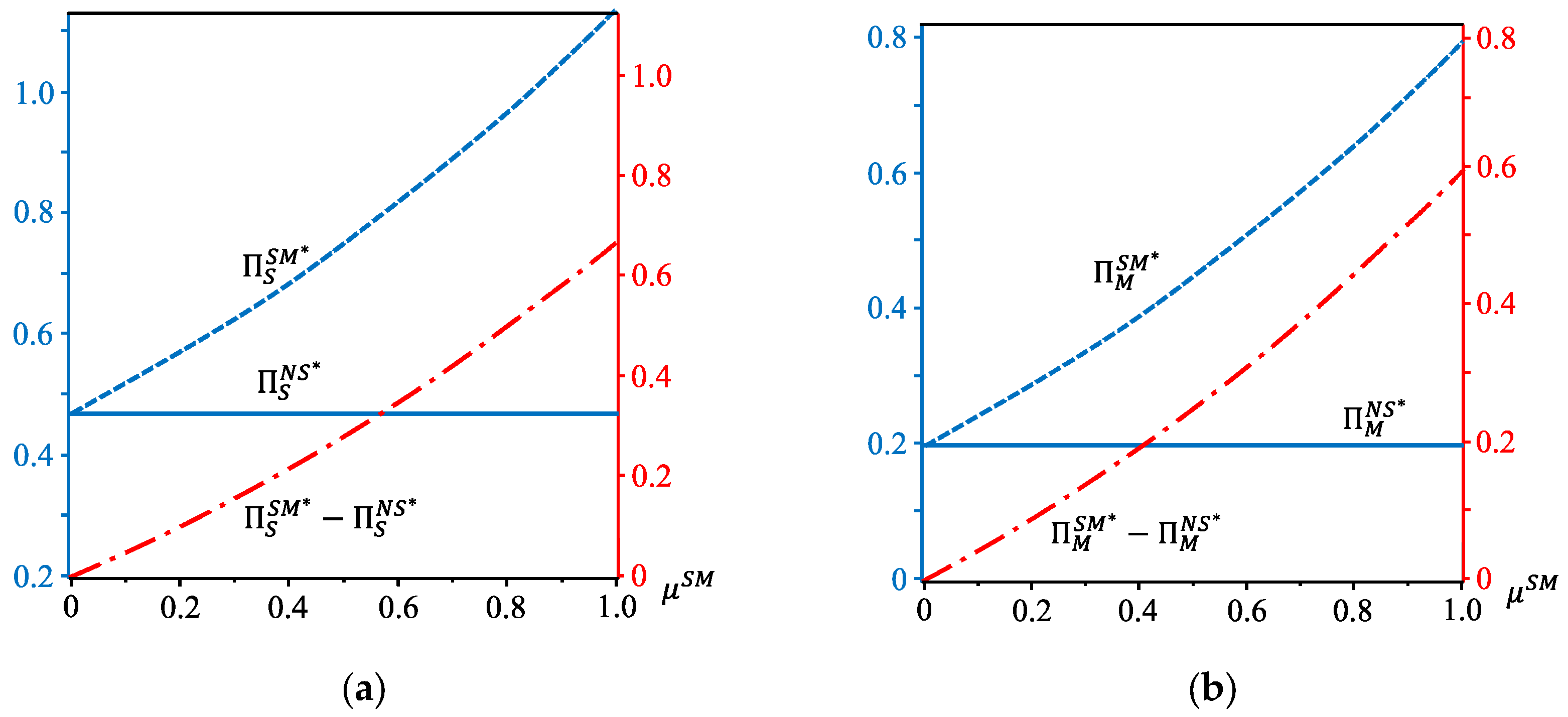
In Figure 5, we can observe that when $K=4$ and $s=0.5$, the change in government subsidy amount will cause an increase in the expected revenues for both the supplier and the manufacturer ($\frac{\partial {\mathsf{\Pi }}_S^{{SM}^{\mathrm{*}}}}{\partial {\mu }^{SM}}>0$ and $\frac{\partial {\mathsf{\Pi }}_M^{{SM}^{\mathrm{*}}}}{\partial {\mu }^{SM}}>0$). As seen from the blue dotted lines in Figure 5a,b, both of them are above their respective solid blue lines, which suggests that their collective revenue with subsidy is greater than that without. The red dotted lines represent the differences between the revenue before and after subsidy, and they are both positive (${\mathsf{\Pi }}_S^{{SM}^{\mathrm{*}}}-{\mathsf{\Pi }}_S^{{NS}^{\mathrm{*}}}>0$ and ${\mathsf{\Pi }}_M^{{SM}^{\mathrm{*}}}-{\mathsf{\Pi }}_M^{{NS}^{\mathrm{*}}}>0$).

Proposition 2.

(a)

${{\mathrm{C}\mathrm{S}}_1^{\mathrm{S}\mathrm{M}}}^{\mathrm{*}}>{{\mathrm{C}\mathrm{S}}_1^{\mathrm{N}\mathrm{S}}}^{\mathrm{*}}$.

(b)

If$\frac{4}{2-\mathrm{s}}<\mathrm{K}<\overline{\mathrm{K}}$,${{\mathrm{C}\mathrm{S}}_2^{\mathrm{S}\mathrm{M}}}^{\mathrm{*}}>{{\mathrm{C}\mathrm{S}}_2^{\mathrm{N}\mathrm{S}}}^{\mathrm{*}}$; if$0<\mathrm{K}<\frac{4}{2-\mathrm{s}}$,${{\mathrm{C}\mathrm{S}}_2^{\mathrm{S}\mathrm{M}}}^{\mathrm{*}}<{{\mathrm{C}\mathrm{S}}_2^{\mathrm{N}\mathrm{S}}}^{\mathrm{*}}$.

According to Table A1, it follows that $\frac{\partial {{CS}_1^{SM}}^{\mathrm{*}}}{\partial {\mu }^{SM}}>0$ which means that the government subsidy can increase the consumer surplus for product 1. Therefore, the consumer surplus of product 1 is better off without the subsidy (${\mu }^{SM}=0$), while the effect of the subsidy on consumer surplus for product 2 is more complicated. Comparing the consumer surplus under strategies NS and SM, we can get ${{CS}_2^{SM}}^{\mathrm{*}}-{{CS}_2^{NS}}^{\mathrm{*}}>0$ if $\frac{4}{2-s}<K<\overline{K}$, which means that the government subsidy increases the consumer surplus for product 2, and ${{CS}_2^{SM}}^{\mathrm{*}}-{{CS}_2^{NS}}^{\mathrm{*}}<0$ if $0<K<\frac{4}{2-s}$, which means that the government subsidy decreases the consumer surplus for product 2.

Proposition 2 states that, compared to strategy $NS$, the consumer surplus for both products 1 and 2 increases under strategy $SM$ only if $\frac{4}{2-s}<K<\overline{K}$. In other words, the consumer surplus increases for all consumers only when the profitability of the technology innovation is high. Interestingly, even when $K$ is low, the supplier will lower the price of product 2, though their consumer surplus remains reduced. From a consumer perspective, buying product 1 is the optimal choice. This indicates to the government’s innovation management that subsidizing new technology via strategy SM can create a win-win situation for all parties ($\frac{4}{2-s}<K<\overline{K}$): it will increase the expected income of the supply-side players (e.g., suppliers and manufacturers) in the supply chain, as well as a net utility from consumers who buy either product 1 or 2.

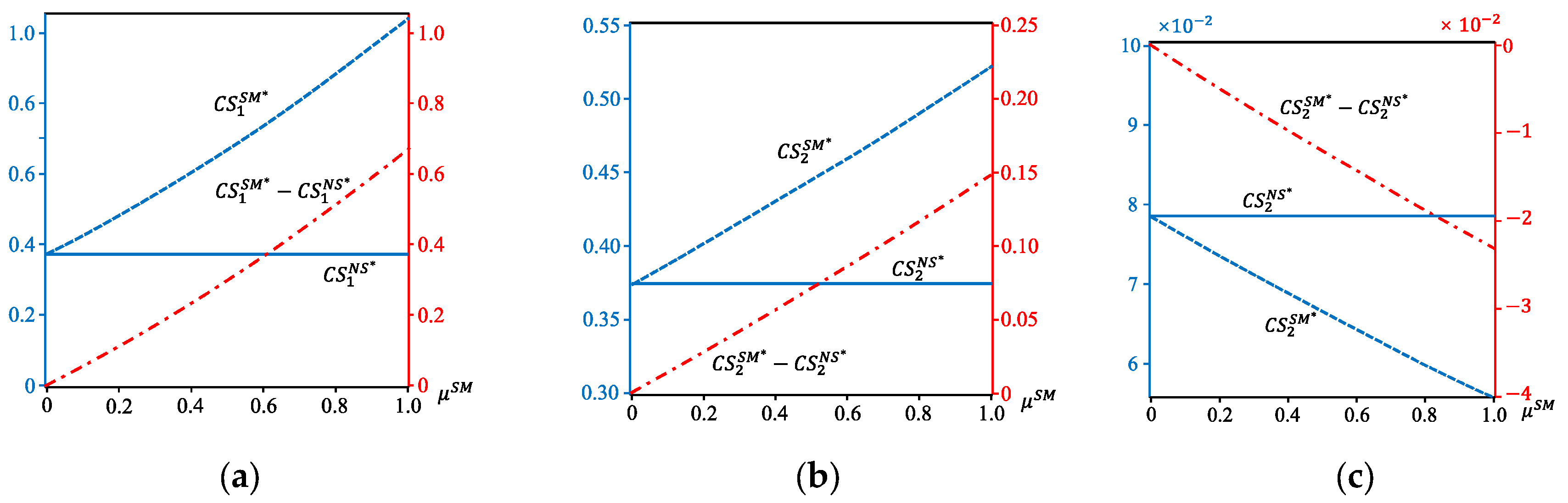
In Figure 6a, when $K=4$ and $s=0.5$, the government subsidy is effective for the consumer surplus for product 1. We can see that the consumer surplus of product 1 is positively influenced by the government subsidy from the blue dotted line ($\frac{\partial {{CS}_1^{SM}}^{*}}{\partial {\mu }^{SM}}>0$), and the subsidized consumer surplus for product 1 is always higher than the unsubsidized consumer surplus (${{CS}_1^{SM}}^{*}-{{CS}_1^{NS}}^{*}>0$). As the consumer surplus of product 2 varies with the amount of government subsidy under different market profitability coefficients of the technological innovation achievement, Figure 6b,c describe the change in the consumer surplus of product 2 when $K=4$ and $K=1.5$, respectively. As can be seen from Figure 6b, when the market profitability of the new technology is high ($K=4$), the changing trend of the consumer surplus of product 2 with the amount of government subsidy is similar to that of product 1. The more government subsidy it receives, the more the consumer surplus of product 2 is. When the market profitability of the new technology is low ($K=1.5$), the more government subsidy it receives, the less the consumer surplus of product 2 is.

4.3. Government Subsidizes the Price of the Supplier’s Product (Strategy $SS$)

If the government chooses to subsidize the supplier’s product with ${\mu }^{SS}$, customers buy products 1 and 2 at the prices of $p_1^{SS}$ and $p_2^{SS}-{\mu }^{SS}$, respectively. The utility of customers who buy product 1 becomes $u_1=\xi +r\tilde{v}{\theta }^{SS}-p_1^{SS}$, and the utility of customers who buy product 2 is $u_2=s\left(\xi +r\tilde{v}{\theta }^{SS}\right)-(p_2^{SS}-{\mu }^{SS})$. The three indifference points of a customer’s reservation price become ${\xi }_1^{SS}=p_1^{SS}-r\tilde{v}{\theta }^{SS}$, ${\xi }_2^{SS}=\frac{(p_2^{SS}-{\mu }^{SS})}{s}-r\tilde{v}{\theta }^{SS}$, and ${\xi }_3^{SS}=\frac{p_1^{SS}-(p_2^{SS}-{\mu }^{SS})}{1-s}-r\tilde{v}{\theta }^{SS}$. With the same reasoning process mentioned above, the demand functions of products 1 and 2 are $q_1^{SS}={\int }_{{\xi }_3^{SS}}^{1}d\xi =1-\frac{p_1^{SS}-(p_2^{SS}-{\mu }^{SS})}{1-s}+r\tilde{v}{\theta }^{SS}$ and $q_2^{SS}={\int }_{{\xi }_2^{SS}}^{{\xi }_3^{SS}}d\xi =\frac{p_1^{SS}-(p_2^{SS}-{\mu }^{SS})}{1-s}-\frac{(p_2^{SS}-{\mu }^{SS})}{s}$. The consumer surpluses of products 1 and 2 are ${CS}_1^{SS}={\int }_{{\xi }_3^{SS}}^1{u}_1^{SS}\left(\xi \right)d\xi =s{q}_1^{SS}{q}_2^{SS}+\frac{1}{2}{q_2^{SS}}^2$ and ${CS}_2^{SS}={\int }_{{\xi }_2^{SS}}^{{\xi }_3^{SS}}{u}_2^{SS}\left(\xi \right)d\xi =\frac{1}{2}s{q_2^{SS}}^2$, respectively. The supplier maximizes his profit (${\mathsf{\Pi }}_S^{SS}$) by setting the target level of innovation (${{\theta }^{SS}}^{\mathrm{*}}$), and the prices of the new technology (${w^{SS}}^{\mathrm{*}}$) and his private brand product ($p_2^{SS}$):

$${\mathsf{\Pi }}_S^{SS}=w^{SS}{q}_1^{SS}+\left(p_2^{SS}-{\mu }^{SS}\right)q_2^{SS}-\frac{c}{\lambda }{{\theta }^{SS}}^2$$

(9)

The manufacturer maximizes her profit (${\mathsf{\Pi }}_M^{SS}$) by setting the price for product 1 (${p_1^{SS}}^{\mathrm{*}}$):

$${\mathsf{\Pi }}_M^{SS}=(p_1^{SS}-w^{SS})q_1^{SS}$$

(10)

The government maximizes social welfare (${\mathsf{\Pi }}_G^{SS}$) by setting the optimal subsidy (${{\mu }^{SS}}^{*}$):

$${\mathsf{\Pi }}_G^{SS}={\mathsf{\Pi }}_S^{SS}+{\mathsf{\Pi }}_M^{SS}+\sum _{i=1}^2{CS}_i^{SS}-{\mu }^{SS}{q}_2^{SS}$$

(11)

Table A1 lists the equilibrium innovation level, quantities, wholesale price, retail prices, and profits. Note that the existence, uniqueness, and stability of these equilibrium results still require $0<K<\overline{K}$ under strategy SS. The condition implies that all these decision variables and expected revenues remain non-negative.

Proposition 3.

(a)

${\Pi }_S^{{SS}^{*}}>{\Pi }_S^{{NS}^{*}}$;

(b)

When $4<K<\overline{K}$, ${\Pi }_M^{{SS}^{*}}>{\Pi }_M^{{NS}^{*}}$; when $0<K<4$, ${\Pi }_M^{{SS}^{*}}>{\Pi }_M^{{NS}^{*}}$ if $0<{\mu }^{SS}<\frac{8(1-s)}{4-K}$and ${\Pi }_M^{{SS}^{*}}<{\Pi }_M^{{NS}^{*}}$if $\frac{8(1-s)}{4-K}<{\mu }^{SS}<p_2$.

Proposition 3 shows that the subsidy strategy is more profitable for the supplier, but its effect on the manufacturer’s ex ante profit is inconclusive. When the market potential of the new technology is high ($4<K<\overline{K}$), a price subsidy for product 2 boosts the manufacturer’s ex ante profit; however, when the market potential of the new technology is low ($0<K<4$), if the subsidy amount is small ($0<{\mu }^{SS}<\frac{8(1-s)}{4-K}$), then it decreases the expected revenue for the manufacturer, and if it is large ($\frac{8(1-s)}{4-K}<{\mu }^{SS}<p_2$), it increases the expected revenue.

Under strategy SS, customers who purchase product 2 will spend less money—thus, the demand for product 2 increases as a result of the government subsidy ($\frac{\partial {q_2^{SS}}^{\mathrm{*}}}{\partial {\mu }^{SS}}=\frac{8-2Ks}{4(8-3s)-(4+s^2)K}>0$). As such, the supplier raises his price for product 2 in response to this increased demand ($\frac{\partial {p_2^{SS}}^{\mathrm{*}}}{\partial {\mu }^{SS}}=\frac{16-2K+(K-2)s}{4(8-3s)-(4+s^2)K}>0$). Moreover, due to the inverse wholesale price effect, the government subsidy influencing product 2’s pricing also causes an increase in the cost of new technologies ($\frac{\partial {w^{SS}}^{\mathrm{*}}}{\partial {\mu }^{SS}}>0$). While the demand for product 1 fluctuates under both the influence of strategy SS and various market competition effects, overall the expected revenue of suppliers steadily rises.

Customers who purchase product 1 will pay the same price as before. When the market profitability of the new technology is high ($4<K<\overline{K}$), even though the government only subsidizes the cost of product 2, demand for product 1 will also rise due to consumers being highly attracted to the new technology ($\frac{\partial {q_1^{SS}}^{\mathrm{*}}}{\partial {\mu }^{SS}}=\frac{2K-8}{4(8-3s)-(4+s^2)K}>0$). In response to this situation, the manufacturer will raise the selling price of product 1 ($\frac{\partial {p_1^{SS}}^{\mathrm{*}}}{\partial {\mu }^{SS}}=\frac{2s+4K-8}{4(8-3s)-(4+s^2)K}>0$) to increase their expected revenue.

When the market profitability of the new technology is low ($0<K<4$), as mentioned in Proposition 1, it is less attractive to consumers, and the number of potential consumers in the market is smaller, so government subsidies have a limited capacity when it comes to stimulating market demand. The main influence of subsidies would be to switch consumers who would normally buy from the manufacturer to the supplier, thus decreasing demand for product 1 and increasing demand for product 2 ($\frac{\partial {q_1^{SS}}^{\mathrm{*}}}{\partial {\mu }^{SS}}<0$, $\frac{\partial {q_2^{SS}}^{\mathrm{*}}}{\partial {\mu }^{SS}}>0$). Intuitively, if the amount of government subsidy is low ($0<{\mu }^{SS}<\frac{8(1-s)}{4-K}$), many customers will still choose product 1, causing the expected revenue growth for its manufacturer to slow. However, if the amount of government subsidy is high ($\frac{8(1-s)}{4-K}<{\mu }^{SS}<p_2$), even though there may be a decrease in demand for product 1 ($\frac{\partial {q_1^{SS}}^{\mathrm{*}}}{\partial {\mu }^{SS}}<0$), the manufacturer can still increase their price to maintain expected revenue growth ($\frac{\partial {p_1^{SS}}^{\mathrm{*}}}{\partial {\mu }^{SS}}>0$). As a result, the total expected revenue of the manufacturer ultimately increases.

In Figure 7, when $s=0.7$, both the supplier’s and the manufacturer’s expected revenue are impacted by the government subsidy strategy SS. Figure 7a,b depict a condition where $K=4.5$, indicating favorable new technology consumer perception. The blue dotted lines depicting the expected revenue slope upwards to the right in both figures, showing that an increase in government subsidy leads to an increased expected revenue for supplier and manufacturer alike. Additionally, the blue dotted lines in both figures are always above their respective solid lines, illustrating that the expected revenue with a subsidy surpasses what it would be without a subsidy. Meanwhile, the red dotted lines display the difference between the expected revenue before and after subsidies, respectively; this trend further confirms that the anticipated returns under a subsidized plan surpass those of an unsubsidized plan. In Figure 7c, where $K=1$ implies a diminished profitability of new technologies, a U-shaped trajectory is exhibited between the manufacturer’s expectation of return on investment and the conferred government subsidy amounts via Figure 7c: when $0<{\mu }^{SS}<\frac{4(1-s)}{4-K}=0.4$ (if $K=1$ and $s=0.7$) (low government subsidies), as price subsidies for product 2 also increase, so do the expectations of a reduced income for the manufacturer; if $\frac{4(1-s)}{4-K}<{\mu }^{SS}<p_2$ (high subsides), increased price support for product 2 is associated with an increasing anticipation of returns for the manufacturer until reaching the threshold $\frac{8(1-s)}{4-K}$ (equal to 0.8 if $K=1$ and $s=0.7$). Beyond this point of return, expectations under subsidization surpass those without it.

Figure 7 illustrates the rule stated in Proposition 3: when the profitability of the new technology is high, the government subsidy increases the expected income of both supplier and manufacturer on the supply side; however, when the profitability is insufficient, the government price subsidy for product 2 can improve the supplier’s expected revenue but its impact on the manufacturer’s expected revenue will depend on the intensity of that price subsidy.

Proposition 4.

(a)

There exists a threshold ${\mu }_{CS}^{SS}=\frac{[2sK\left(3s-8\right)-8(2s^2-11s+4\left)\right]}{\left(4-K\right)[\left(1-s\right)K-2(6-s\left)\right]}$, ${{CS}_1^{SS}}^{*}>{{CS}_1^{NS}}^{*}$ if $0<{\mu }^{SS}<{\mu }_{CS}^{SS}$, ${{CS}_1^{SS}}^{*}<{{CS}_1^{NS}}^{*}$ if ${\mu }_{CS}^{SS}<{\mu }^{SS}<p_2$;

(b)

${{CS}_2^{SS}}^{*}>{{CS}_2^{NS}}^{*}$.

Part (a) of Proposition 4 indicates an important distinction between the case where the government subsidizes the price of product 1 and the case where it subsidizes the price of product 2. In the former, the consumer surplus for product 1 will always improve; however, for the latter, the consumer surplus for product 1 will depend on the amount of the subsidy. If the subsidy amount is low, the consumer surplus of product 1 will still rise. But if it is high, then the consumer surplus of product 1 will decrease. Part (b) of Proposition 4 is in line with the intuition that subsidizing the price of product 2 will increase the consumer surplus for product 2.

The government needs to set reasonable price subsidies in the process of innovation management, as this will result in an increased consumer surplus for both subsidized and unsubsidized products. If the subsidy amount is too high, it can lead to a suppression of subsidized products against those that are unsubsidized, resulting in an increase in the surplus of consumers who buy subsidized products and a decrease in the surplus of those buying unsubsidized products.

Conventional wisdom claims that when a government subsidizes the price of a product, it will lead to a decrease in the consumer surplus of competitive offerings. This view fails to consider the potential spillover benefits that such subsidies would have. By combining Propositions 2 and 4, it is clear that different policy approaches to pricing subsidies can have drastically different effects on the consumer surplus. When the government subsidizes prices for manufacturers’ products, to increase the overall consumer surplus, the focus must shift towards the market profitability of new technologies being developed by these firms. Alternatively, if supplier-end-price subsidies are utilized, policy-makers must strive to formulate equitable price subsidy structures to promote an increase in consumer welfare.

Figure 8 describes the different influences of a subsidy (SS) on the consumer surplus of products 1 and 2. To make the graph more readable, let $K=2$ and $s=0.4$ within the limits of constraints. In Figure 8a, the blue dotted line represents the change in the consumer surplus for product 1 with regard to the amount of the subsidy. The government’s price subsidy for product 2 has an inverted-U shaped effect on the consumer surplus for product 1: when the subsidy amount is low ($0<{\mu }^{SS}<\frac{16+\left(8-3K\right)s^2-(44-8K)s}{\left(4-K\right)[\left(K-2\right)s+12-K]}=0.25$, if $K=2$ and $s=0.4$), the consumer surplus increases; however, when it is high ($0.25<{\mu }^{SS}<p_2$), the consumer surplus decreases. If it reaches a certain threshold (${\mu }_{CS}^{SS}=0.512$, if $K=2$ and $s=0.4$), with further increases in the subsidy amount, the consumer surplus begins to fall below that without subsidies. In Figure 8b, the blue dotted line represents the consumer surplus for product 2 and its increase with additional subsidization; the consumer surplus for the subsidized product 2 is always above that without subsidies (which is represented by the blue solid line). The government subsidy of product 2’s price, therefore, has a steady positive effect on its consumer surplus.

4.4. Government Subsidizes the Cost of the Supplier’s Innovation (Strategy $SC$)

Under this circumstance, customers buy products 1 and 2 at the price of $p_1^{SC}$ and $p_2^{SC}$, respectively. The utility functions, demand functions, and the three indifference points are the same as in Section 4.1. The only difference is that the cost of the supplier’s innovation becomes $(1-{\tau }^{SC})\frac{c}{\lambda }{{\theta }^{SC}}^2$. Therefore, the supplier maximizes his profit (${\mathsf{\Pi }}_S^{SC}$) by setting the target level of the innovation (${{\theta }^{SC}}^{*}$) and the price of the new technology (${w^{SC}}^{*}$):

$${\mathsf{\Pi }}_S^{SC}=w^{SC}{q}_1^{SC}+p_2^{SC}{q}_2^{SC}-\left(1-{\tau }^{SC}\right)\frac{c}{\lambda }{{\theta }^{SC}}^2$$

(12)

The manufacturer maximizes her profit (${\mathsf{\Pi }}_M^{SC}$) by setting the price for product 1 (${p_1^{SC}}^{*}$):

$${\mathsf{\Pi }}_M^{SC}=(p_1^{SC}-w^{SC})q_1^{SC}$$

(13)

The government maximizes social welfare (${\mathsf{\Pi }}_G^{SC}$) by setting the optimal subsidy (${{\tau }^{SC}}^{*}$):

$${\mathsf{\Pi }}_G^{SC}={\mathsf{\Pi }}_S^{SC}+{\mathsf{\Pi }}_M^{SC}+\sum _{i=1}^2{CS}_i^{SC}-{\tau }^{SC}\frac{c}{\lambda }{{\theta }^{SC}}^2$$

(14)

Table A1 lists the equilibrium innovation level, quantities, wholesale price, retail prices, and profits. Note that under strategy SC, the existence, uniqueness, and stability of these equilibrium results still require $0<K<\stackrel{̿}{K}$, where $\stackrel{̿}{K}=\frac{4\left(8-3s\right)}{4+s^2}(1-{\tau }^{SC})$. The condition implies that all these decision variables and expected revenues remain non-negative.

Proposition 5.

${\Pi }_S^{{SC}^{*}}>{\Pi }_S^{{NS}^{*}}$ and ${\Pi }_M^{{SC}^{*}}>{\Pi }_M^{{NS}^{*}}$.

According to the equilibrium profits of the supplier and manufacturer in Table A1, it is evident that $\frac{\partial {\mathsf{\Pi }}_S^{{SC}^{\mathrm{*}}}}{\partial {\mu }^{SC}}>0$ and $\frac{\partial {\mathsf{\Pi }}_M^{{SC}^{\mathrm{*}}}}{\partial {\mu }^{SC}}>0$. ${\mu }^{SC}=0$ stands for when the government does not subsidize the technology innovation. It follows that if the government subsidizes the innovation cost of the supplier, both parties will bring in more ex ante profit than without any form of subsidy from the government.

It can be seen from Table A1 that the government’s subsidy to the supplier’s innovation costs will affect the equilibrium decisions of each subject in the supply chain in a different way, thus affecting their expected income. According to $\frac{\partial {q_1^{SC}}^{*}}{\partial {\tau }^{SC}}=\frac{8(1-s)(4+s^2)K}{{\left[4\left(8-3s\right)\right(1-{\tau }^{SC})-(4+s^2\left)K\right]}^2}>0$, $\frac{\partial {q_2^{SC}}^{*}}{\partial {\tau }^{SC}}=\frac{2(6-s)(4+s^2)K}{{\left[4\left(8-3s\right)\right(1-{\tau }^{SC})-(4+s^2\left)K\right]}^2}>0$, we can see that the demand of both the manufacturer’s and the supplier’s products will increase with the cost subsidy. Contrary to our intuition, note that $\frac{\partial {p_1^{SC}}^{*}}{\partial {\tau }^{SC}}=\frac{2(2-s)(6-s)(4+s^2)K}{{\left[4\left(8-3s\right)\right(1-{\tau }^{SC})-(4+s^2\left)K\right]}^2}>0$ and $\frac{\partial {p_2^{SC}}^{*}}{\partial {\tau }^{SC}}=\frac{2s(6-s)(4+s^2)K}{{\left[4\left(8-3s\right)\right(1-{\tau }^{SC})-(4+s^2\left)K\right]}^2}>0$, the equilibrium price of product 1 and 2 will increase, although the government cost subsidy is lower than the innovation cost of the upstream supplier. Combined with $\frac{\partial {w^{SC}}^{*}}{\partial {\tau }^{SC}}=\frac{2(s^2-4s+8)(4+s^2)K}{{\left[4\left(8-3s\right)\right(1-{\tau }^{SC})-(4+s^2\left)K\right]}^2}>0$, it is easy to derive that the manufacturer’s and the supplier’s profit will increase with the cost subsidy. Given the trend of demand and price with respect to the cost subsidy, the consumer surplus of both kinds of products will also increase.

In Figure 9, when $K=1$ and $s=0.5$, the impact of government cost subsidies of the suppliers’ innovation activity on the supplier’s and the manufacturer’s expected revenue is visualized. The blue dotted lines in Figure 9 demonstrate the supplier’s and the manufacturer’s expected revenue when subsidies are provided; these increase with the government subsidy amount. The solid blue lines in Figure 9a,b indicate the supplier’s and the manufacturer’s expected revenue without subsidy; both of these lines are below the blue dotted line, illustrating that the unsubsidized expected revenue is always lower than the subsidized situations. The red dotted lines pinpoint the difference between subsidized and unsubsidized situations, and also show an increasing trend.

Proposition 6.

${{CS}_1^{SC}}^{*}>{{CS}_1^{NS}}^{*}$and ${{CS}_2^{SC}}^{*}>{{CS}_2^{NS}}^{*}$.

According to Table A1, it follows that $\frac{\partial {{CS}_1^{SC}}^{\mathrm{*}}}{\partial {\mu }^{SC}}>0$ and $\frac{\partial {{CS}_2^{SC}}^{\mathrm{*}}}{\partial {\mu }^{SC}}>0$ which means that both of the consumer surpluses for products 1 and 2 will increase with the government cost subsidy. Therefore, the consumer surpluses of products 1 and 2 are better off without subsidy (${\mu }^{SC}=0$).

Comparing Propositions 2, 4, and 6 reveals a significant difference in the impact of price and cost subsidies on consumer surplus at the consumer end of a supply chain. When the government subsidizes the price of a product, it may increase the consumer surplus of that particular product; however, this can also reduce the consumer surplus of other unsubsidized products. In contrast, subsidizing the innovation cost of suppliers directly leads to an expansion of the total market size ($\frac{\partial {q_1^{SC}}^{\mathrm{*}}}{\partial {\tau }^{SC}}>0$, $\frac{\partial {q_2^{SC}}^{\mathrm{*}}}{\partial {\tau }^{SC}}>0$). Consumers who were not ready to purchase will now choose to buy products featuring new technologies brought about by government subsidies. Consequently, both products will benefit from an increase in the consumer surplus.

In Figure 10, both product 1’s and product 2’s consumer surplus increase as the amount of government cost subsidy increases. The blue dotted lines in Figure 10a,b represent the consumer surpluses of products 1 and 2, respectively. Not only do they tend to move towards the upper right corner, but they also stay above the solid blue lines, indicating that the subsidized consumer surpluses are always greater than their unsubsidized counterparts.

Table 2. Changes in the expected revenue and consumer surplus (different subsidy strategy vs. no subsidy).

Subsidy Strategy	Strategy SM	Strategy SS	Strategy SC
Supplier’s expected revenue	↑	↑	↑
Manufacturer’s expected revenue	↑	↓↑	↑
Product 1’s consumer surplus	↑	↓↑	↑
Product 2’s consumer surplus	↓↑	↑	↑

Where: ↑ means that the variable will increase compared to the scenario under strategy NS; ↓↑ means that compared to the scenario under subsidy strategy NS, the variable may either increase or decrease.

summarizes the research findings in this subsection. The three columns on the right side of the table represent the three subsidy strategies employed by the government, namely, strategy SM, SS, and SC. The subsequent four rows represent the expected profits of the supplier and the manufacturer, and the consumer surplus for product 1 (the manufacturer’s product) and product 2 (the supplier’s product). The upward arrows in the table indicate an increase in the variable compared to the non-subsidized scenario, while double-headed arrows indicate a variable that may either increase or decrease compared to the non-subsidized scenario. For instance, in Table 2, the upward arrow in the second row and second column signifies that the government subsidizing the price of the manufacturer’s product (strategy SM) would lead to an increase in the expected revenue of the supplier compared to the non-subsidized scenario. The double-headed arrow in the fourth row and third column indicates that when the government subsidizes the price of the supplier’s product (strategy SS), the consumer surplus for purchasing product 1 may either increase or decrease.

Based on Table 2, it becomes evident that government subsidy policies have distinct impacts on the expected returns of the supplier and the manufacturer when the supplier encroaches into the manufacturer’s product market. Specifically, price subsidies by the government to the manufacturer’s product increase the expected returns for both the supplier and the manufacturer. Likewise, subsidies to the innovation costs of the supplier exhibit a similar trend. However, when the government applies price subsidies to the products of the supplier, it elevates the expected returns for the supplier but introduces uncertainty in its effects on the expected returns of the manufacturer. This contrast aligns with distinctions observed in the existing body of literature. For instance, Huang et al.’s research revealed that, irrespective of the government’s subsidy policy, profits for both manufacturers and retailers rise with increasing subsidy rates [9]. Nie et al. noted that when the government subsidizes one company, the expected returns of the subsidized firm increase, while the expected returns of non-subsidized firms decrease [25]. The primary variance between these studies and our findings in this paper pertains to the inconsistency in market competition relations. Thus, it is evident that different market competition relations lead to varying impacts of government subsidies on the expected returns of firms.

Furthermore, it is apparent that government subsidies have different effects on consumer surplus for different products. Under price subsidy strategies, the consumer surplus for the products of subsidized firms increases, while the consumer surplus for products from non-subsidized firms may either increase or decrease. Under cost subsidy strategies, the consumer surplus for both types of products increases. In contrast to the conclusions of the existing literature, it is noticeable that when supply chain encroachment is not considered, the existing literature generally indicates that subsidies, whether internal to the supply chain [66] or government-sponsored [22], lead to an enhancement of the consumer surplus.

5. Government’s Optimal Innovation Subsidy Strategy Decision

In Section 4, we discussed the changes in expected revenue and consumer surplus at both the supply end (i.e., the supplier and the manufacturer) and consumption end (i.e., products 1 and 2). We analyzed the results of our models to reveal the influence mechanism of government subsidies on innovation activities. However, the optimal method for the government to select a subsidy strategy when a supplier encroaches upon the supply chain remains unexplored. This will be the focal point of analysis in this section.

Lemma 1.

There exist three thresholds

${\mathrm{K}}^{\mathrm{S}\mathrm{M}}=\frac{4({\mathrm{s}}^2+2\mathrm{s}-4+2\sqrt{-2{\mathrm{s}}^4+4{\mathrm{s}}^3+2{\mathrm{s}}^2-8\mathrm{s}+4})}{\mathrm{s}(3{\mathrm{s}}^2-4)}$,

${\mathrm{K}}^{\mathrm{S}\mathrm{S}}=\frac{3{\mathrm{s}}^3-6{\mathrm{s}}^2+36\mathrm{s}-32+\sqrt{9{\mathrm{s}}^6+36{\mathrm{s}}^5-152{\mathrm{s}}^3+256{\mathrm{s}}^2+768\mathrm{s}}}{2{\mathrm{s}}^3+3{\mathrm{s}}^2+8\mathrm{s}-4}$,

${\mathrm{K}}^{\mathrm{S}\mathrm{C}}=\frac{8(9{\mathrm{s}}^2-48\mathrm{s}+64)}{3{\mathrm{s}}^3-4{\mathrm{s}}^2-36\mathrm{s}+112}$,

(a)

${\Pi }_G^{{SM}^{*}}>{\Pi }_G^{{NS}^{*}}$ if $0<K<K^{SM}$, otherwise ${\Pi }_G^{{SM}^{*}}<{\Pi }_G^{{NS}^{*}}$;

(b)

${\Pi }_G^{{SS}^{*}}>{\Pi }_G^{{NS}^{*}}$ if $0<K<K^{SS}$, otherwise ${\Pi }_G^{{SS}^{*}}<{\Pi }_G^{{NS}^{*}}$;

(c)

${\Pi }_G^{{SC}^{*}}>{\Pi }_G^{{NS}^{*}}$ if $0<K<K^{SC}$, otherwise ${\Pi }_G^{{SC}^{*}}<{\Pi }_G^{{NS}^{*}}$.

Lemma 1 demonstrates that each subsidy strategy has its own applicable scope. When implemented in the proper realm, innovation subsidies can drastically improve social welfare; if, however, they are applied outside of the appropriate boundaries, they will lead to a decrease in social welfare. Specifically, when the profitability coefficient for the new technology is within a certain range $\mathrm{o}\mathrm{f} 0<K<K^{SM}$, then offering a price subsidy for product 1 will increase the overall social welfare; if the profitability coefficient falls outside of that range, then the subsidy will result in a reduction in social welfare. The applicable scope of the subsidy strategy $SS$ is $0<K<K^{SS}$, and the applicable scope of the subsidy strategy $SC$ is $0<K<K^{SC}$. Noting that all boundary conditions are functions of $K$ with respect to $s$, it is clear that the applicable conditions of the government subsidies lie heavily on both the new technology’s profitability coefficient ($K$) and the intensity of market competition ($s$).

Figure 11 plots the feasible eligibility conditions for different types of subsidy strategies. In Figure 11, the red lines (including the red solid line and the red dashed line) delineate the boundary conditions ($K=\overline{K}$ and $K=\stackrel{̿}{K}$) for technological innovation. Supplier-initiated innovation activities must remain within these boundaries to yield positive expected revenue. The blue line (including the blue dotted line, the blue dashed line, and the blue dot-dash line) indicate the boundary conditions of different government subsidies ($K=K^{SM}$ for strategy $SM$, $K=K^{SS}$ for strategy $SS$, and $K=K^{SC}$ for strategy $SC$). Only when the government subsidizes within these boundary conditions will social welfare increase.

From Figure 11, we can derive an understanding: namely, cost subsidies necessitate a lesser degree of government insight into innovation activities and market competitiveness compared to what is required for price subsidies. The government can directly determine whether to provide cost subsidies to technology suppliers based on their intention to engage in technological innovation activities. With $K^{SC}=\stackrel{̿}{K}$, this indicates that whenever a technology supplier engages in specific technological innovation (i.e., when the innovation activity ensures positive expected returns for the supplier, meeting the condition of $K<\stackrel{̿}{K}$), the government can provide cost subsidies (also fulfilling $K<K^{SC}$). Moreover, given $K^{SM}<\overline{K}$ and $K^{SS}<\overline{K}$, it follows that while a supplier’s innovation efforts may result in positive expected income ($K<\overline{K}$), it does not necessarily warrant the government’s implementation of price subsidies, as the government’s price subsidy might adversely impact social welfare if $K^{SM}<K<\overline{K}$ or $K^{SS}<K<\overline{K}$.

Additionally, the area of relevance for price subsidies concerning product 1 is primarily focused on the lower left corner. This signifies that its subsidy strategy for manufacturers is more extensively employed in scenarios with lower competition levels. Conversely, the area applicable for price subsidies regarding product 2 is concentrated in the lower right corner, indicating a prevalence of its subsidy strategy towards suppliers in situations characterized by higher competition levels.

Lemma 1 analyzed the implementation conditions of the three subsidy strategies from the perspective of whether social welfare is improved before and after their implementation, but did not make a horizontal comparison between them. The applicable conditions of the three strategies overlap considerably: in Region Ⅰ, shown in Figure 10 ($0<s<1$ and $0<K<\mathrm{m}\mathrm{i}\mathrm{n}\{K^{SM},K^{SS}\}$), all three can be adopted; in Region Ⅱ, both SS and SC can be used; and in Region Ⅲ, both SM and SC are available. In such an environment where various subsidy strategies can be implemented, further analysis is necessary to determine which one would be the most appropriate choice.

Lemma 2.

In the region Ⅰ that $0<s<1$ and $0<K<min\{K^{SM},K^{SS}\}$,

(a)

When $0<s<0.9610$, then ${\Pi }_G^{{SM}^{*}}>{\Pi }_G^{{SC}^{*}}$;

(b)

When $0.9610<s<1$, ${\Pi }_G^{{SM}^{*}}>{\Pi }_G^{{SC}^{*}}$if $0<K<K_1$; ${\Pi }_G^{{SM}^{*}}>{\Pi }_G^{{SC}^{*}}$if $K_1<K<K^{SS}$.

where $K_1=-\frac{2\left(3s^3-40s^2+156s-144\right)}{s\left(8s^3-35s^2+16s+36\right)}$.

According to Lemma 2, in the region that $0<s<1$ and $0<K<\mathrm{m}\mathrm{i}\mathrm{n}\{K^{SM},K^{SS},K_1\}$, the relationship ${\mathsf{\Pi }}_G^{{SM}^{*}}>{\mathsf{\Pi }}_G^{{SC}^{*}}$ always exists, which means that in this region, the government choosing to subsidize the manufacturer’s product can achieve greater social welfare than subsidizing the cost of the supplier’s innovative activities. In the region that $0<s<1$ and $K_1<K<K^{SS}$, ${\mathsf{\Pi }}_G^{{SM}^{*}}<{\mathsf{\Pi }}_G^{{SC}^{*}}$, which means that in this region, subsidizing the cost of the supplier’s innovation activities will achieve greater social welfare than subsidizing the price of the manufacturer’s product.

Lemma 3.

In the region Ⅰ that $0<s<1$ and $0<K<min\{K^{SM},K^{SS}\}$,

(a)

${\Pi }_G^{{SM}^{*}}>max\{{\Pi }_G^{{SS}^{*}}, {\Pi }_G^{{SC}^{*}}\}$ if $0<K<min\{K^{SM},K_2\}$;

(b)

${\Pi }_G^{{SS}^{*}}>{\Pi }_G^{{SM}^{*}}>{\Pi }_G^{{SC}^{*}}$ if $K_2<K<min\{K^{SS},K_1\}$;

(c)

${\Pi }_G^{{SS}^{*}}>{\Pi }_G^{{SC}^{*}}>{\Pi }_G^{{SM}^{*}}$ if $K_1<K<K^{SS}$.

where $K_2=\frac{(s-6)(-23s^3+58s^2-44s+8+\sqrt{-47s^6+500s^5-1556s^4+1056s^3+2736s^2-4800s+2112})}{2(6s^4-19s^3+20s^2+4s-16)s}$

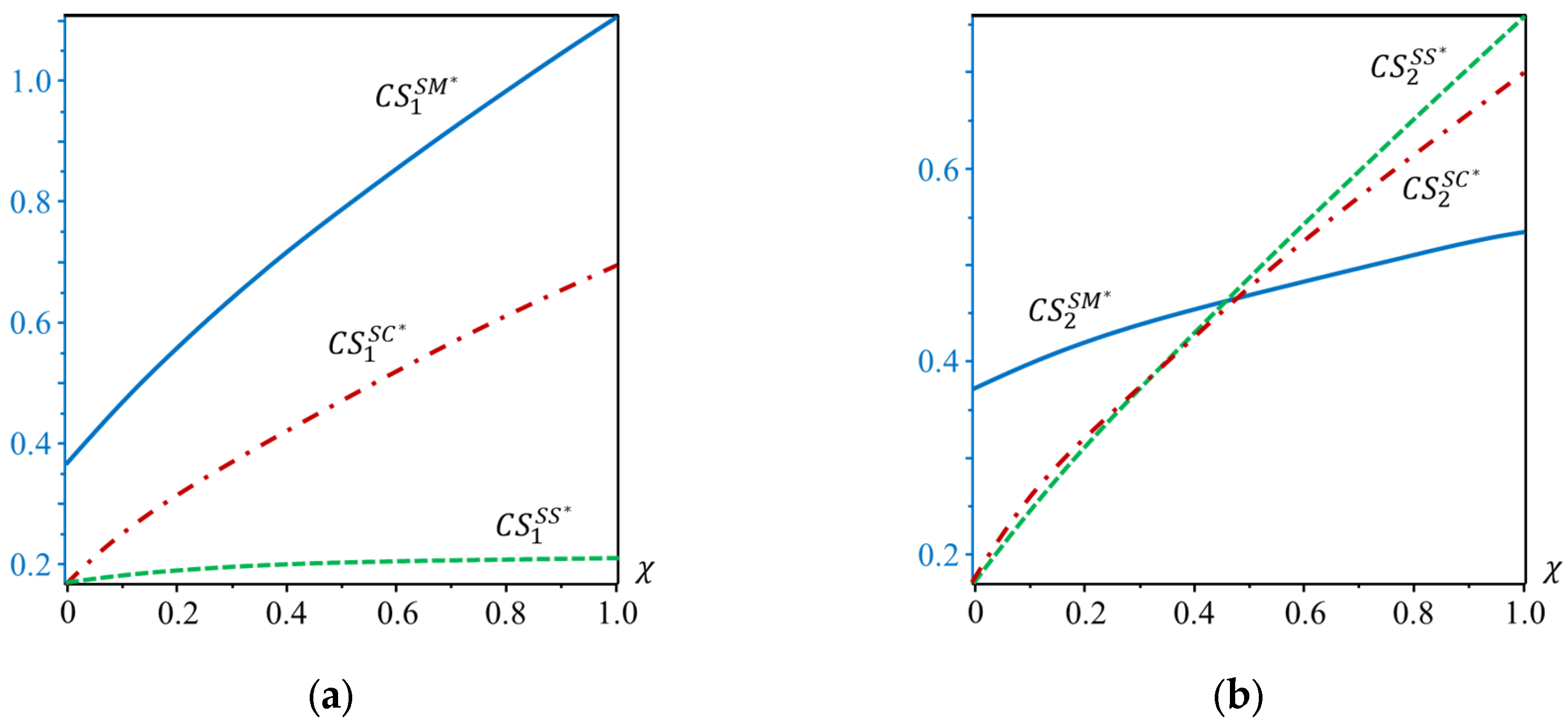
Region I in Figure 10 is analyzed by Lemmas 2 and 3. Although all three subsidy strategies in region Ⅰ can increase social welfare, the extent of the increase is not the same. When $0<K<\mathrm{m}\mathrm{i}\mathrm{n}\{K^{SM},K_2\}$, the increment of social welfare brought by the price subsidy of product 1 is the largest, followed by the price subsidy of product 2, and then the subsidy to the innovation cost of the supplier. When $K_2<K<\mathrm{m}\mathrm{i}\mathrm{n}\{K^{SS},K_1\}$, the social welfare increment generated by subsidy strategy SS is the largest, followed by subsidy strategy SM, and then subsidy strategy SC. When $K_1<K<K^{SS}$, subsidy strategy SS produces the largest increment of social welfare, followed by subsidy strategy SC and subsidy strategy SM. In summary, in region Ⅰ, if $0<K<\mathrm{m}\mathrm{i}\mathrm{n}\{K^{SM},K_2\}$, then the government should choose subsidy strategy SM; if $K_2<K<K^{SS}$, then the government should choose subsidy strategy SS.

Lemma 4.

In the region Ⅱ that $0<s<0.8279$ and $K^{SM}<K<min\{K^{SS},K^{SC}\}$,

(a)

${\Pi }_G^{{SS}^{*}}>{\Pi }_G^{{SC}^{*}}$, if $0<s<0.6622$;

(b)

When $0.6622<s<0.6800$, ${\Pi }_G^{{SS}^{*}}>{\Pi }_G^{{SC}^{*}}$ if $K_3<K<K^{SC}$, ${\Pi }_G^{{SC}^{*}}>{\Pi }_G^{{SS}^{*}}$ if $K^{SM}<K<K_3$;

(c)

${\Pi }_G^{{SC}^{*}}>{\Pi }_G^{{SS}^{*}}$ if $0.6800<s<0.8279$.

where $K_3=\frac{9s^3(s^2-12s+36)}{6s^6-59s^5+116s^4+246s^3-456s^2-216s+288}$

In Region Ⅱ of Figure 6, both subsidy strategies SS and SC can increase social welfare. However, the increment brought by the two subsidy strategies is not the same. Lemma 4 compares the increment. The analysis shows that when $0<\mathrm{s}<0.6800$ and $\mathrm{m}\mathrm{a}\mathrm{x}\{K^{SM},K_3\}<K<K^{SC}$, subsidy strategy SS can produce a larger increment of social welfare; when $0.6622<\mathrm{s}<0.8279$ and $K^{SM}<K<\mathrm{m}\mathrm{i}\mathrm{n}\{K_3,K^{SS}\}$, subsidy strategy SC can produce a larger increment of social welfare.

Lemma 5.

In the region Ⅲ that $0.8279<s<1$ and $K^{SS}<K<min\{K^{SM},K^{SC}\}$,

(a)

When $0.8279<s<0.8719$, ${\Pi }_G^{{SM}^{*}}>{\Pi }_G^{{SC}^{*}}$;

(b)

When $0.8719<s<0.9609$, ${\Pi }_G^{{SM}^{*}}>{\Pi }_G^{{SC}^{*}}$ if $K^{SS}<K<K_1$, ${\Pi }_G^{{SC}^{*}}>{\Pi }_G^{{SM}^{*}}$ if $K_1<K<K^{SC}$;

When $0.9609<s<1$, ${\Pi }_G^{{SC}^{*}}>{\Pi }_G^{{SM}^{*}}$.

In Region Ⅲ in Figure 10, the government can choose subsidy strategies SM and SC. Although both kinds of strategies can increase social welfare, the increment is not the same. From Lemma 5 we know that when $0.8279<\mathrm{s}<0.9609$ and $K^{SS}<K<\mathrm{m}\mathrm{i}\mathrm{n}\{K^{SM},K_1\}$, the social welfare increment generated by subsidy strategy SM is larger; when $0.8719<\mathrm{s}<1$ and $\mathrm{m}\mathrm{a}\mathrm{x}\{K^{SS},K_1\}<K<K^{SC}$, the social welfare increment generated by strategy SC is larger.

From Lemma 1 to Lemma 5 we can obtain Proposition 7.

Proposition 7.

When the supplier encroaches the supply chain, the government’s optimal choices of innovation subsidies are as follows:

(a)

No subsidy is the optimal choice if $\mathit{max}\left\{K^{SM}, K^{SS}, K^{SC}\right\}<K<\overline{K}$;

(b)

Subsidy strategy SM is the optimal choice if $0<K<min\{K^{SM},{ K}_2\}$ or $0.8279<s<0.9609$ and $K^{SS}<K<min\{K^{SM},{ K}_1\}$ or $K^{SC}<K<K^{SM}$;

(c)

Subsidy strategy SS is the optimal choices if $0<s<0.6800$ and $max\{K^{SM},{ K}_3\}<K<K^{SS}$ or $0.8279<s<1$ and $K_2<K<K^{SS}$;

(d)

Subsidy strategy SC is the optimal choice if $0.6622<s<0.8719$ and $K^{SM}<K<min\{K_3, K^{SC}\}$ or $0.8719<s<1$ and $max\{K^{SS},K_1\}<K<K^{SC}$.

To have an intuitive understanding of the applicable conditions of different subsidy strategies, according to Proposition 7, this paper plots the distribution regions of different government subsidy strategies, as seen in Figure 12. Firstly, the government is not encouraged to subsidize innovation activities in any form if the market profitability coefficient is large enough ($\max \left\{K^{SM}, K^{SS}, K^{SC}\right\}<K<\overline{K}$), as shown in the light grey area in Figure 12—this would lead to a decline in social welfare.

Secondly, subsidy strategy SM is mainly applied to situations where the market profitability of the new technology is low ($0<K<\mathrm{m}\mathrm{i}\mathrm{n}\{K^{SM},{ K}_2\}$). As the area filled by the diagonal stripes in Figure 12 shows, under such circumstances the new technology has not yet been recognized by most consumers in the market. This may be due to a lack of consumer awareness or undeveloped relevant consumer needs. Therefore, the primary purpose of government intervention is to aid manufacturers in developing the market for this technology. Compared to upstream suppliers, manufacturers possess complete sales channels and accurate and plentiful market information. Through price subsidies for product 1, manufacturers can fully utilize their channel advantages and make more customers aware of this technology while fostering the market.

Third, subsidy strategy SS is applicable under two circumstances. When the market profitability of the new technology is high ($\mathrm{m}\mathrm{a}\mathrm{x}\{K^{SM},{ K}_3\}<K<K^{SS}$), i.e., the new technology is favoured by the majority of consumers, and the supplier’s and manufacturer’s products are vastly different ($0<\mathrm{s}<0.6800$), either belonging to different product categories (i.e., tablets & laptops), or targeted at different niches (e.g., the elderly or women), this creates an atmosphere where there is no intense competition between these two parties, and a strong market prospect offers a foundation for expansion. A government subsidy for the supplier’s products helps cultivate this product market, which leads to both parties growing their respective markets, subsequently improving social welfare. The second scenario is when the market profitability of the new technology is relatively low ($K_2<K<K^{SS}$), and there is a highly substitutable supplier-manufacturer product market ($0.8279<\mathrm{s}<1$). In the area filled with a lattice pattern in the lower right corner of Figure 12, not only does the new technology lack acceptance among consumers but it also has a largely uncertain future with immense competition. Here, the government subsidies, as a signaling mechanism, can enhance the market acceptance of the new technologies. Simultaneously, subsidies can assist suppliers in overcoming intense market competition through continuous technological innovation.

Finally, the analysis in Section 4 demonstrates that the subsidy on supplier development costs has a widely applicable scope. Yet, our analysis found that, in most cases, this cost subsidy does not result in the greatest social welfare increment. It is only when the market competition is intense and the new technology’s market profitability factor is relatively high that the subsidy will lead to a significant increase in social welfare; this is illustrated by the area filled with vertical stripes in Figure 12.

6. Extensions and Discussions

In this section, we broaden the model to encompass additional scenarios for examining and deliberating upon our primary insights. Section 6.1 delves into instances where the supplier and the manufacturer come from different countries. Section 6.2 addresses situations where budget constraints impose limitations on government subsidies. Through these expanded analyses, we aim to effectively validate the applicability and robustness of the research findings from an alternative perspective.

6.1. The Supplier and the Manufacturer Come from Different Countries

When the supplier and manufacturer come from different countries, we assume that, in reality, the government only subsidizes the product or innovation costs of a domestic enterprise. When the manufacturer is local but the technology supplier is foreign, the government has two subsidy strategies: either no price subsidy (strategy MNS, where the first M denotes the manufacturer being local) or a price subsidy for the manufacturer’s product (strategy MSM). When the technology supplier is domestic but the product manufacturer is foreign, the government has three subsidy strategies: no subsidy (strategy SNS, where the first S denotes the supplier being local), a price subsidy for the supplier’s product (strategy SSS), or a subsidy for the supplier’s innovation costs (strategy SSC). As the structure of the supply chain remains unchanged and the revenue sources for the supplier and manufacturer remain constant, the functions for the expected profit of the supplier and manufacturer also remain unchanged. However, since the government’s expected revenue is represented using social welfare, which includes the expected profit of the supplier and manufacturer, consumer surplus, and subtracting government subsidy expenditure, the expected revenue function for the government changes when either the manufacturer or the technology supplier is a foreign enterprise. For instance, when the technology supplier is foreign, the government’s expected revenue no longer includes the expected profit of the technology supplier. The expected revenue functions for the government under the aforementioned subsidy strategies are detailed in

Table 3. Government expected revenue function under different subsidy strategies when suppliers and manufacturers come from different countries.

The National Situation of Each Subject	Subsidy Strategy	The Government’s Expected Revenue
A domestic manufacturer and a foreign supplier	$\mathrm{Strategy} MNS$	${\mathsf{\Pi }}_G^{MNS}={\mathsf{\Pi }}_M^{MNS}+{\displaystyle \sum _{i=1}^2}{CS}_i^{MNS}$
	$\mathrm{Strategy} MSM$	${\mathsf{\Pi }}_G^{MSM}={\mathsf{\Pi }}_M^{MSM}+{\displaystyle \sum _{i=1}^2}{CS}_i^{MSM}-{\mu }^{MSM}{q}_1^{MSM}$
A domestic supplier and a foreign manufacturer	$\mathrm{Strategy} SNS$	${\mathsf{\Pi }}_G^{SNS}={\mathsf{\Pi }}_S^{SNS}+{\displaystyle \sum _{i=1}^2}{CS}_i^{SNS}$
	$\mathrm{Strategy} SSS$	${\mathsf{\Pi }}_G^{SSS}={\mathsf{\Pi }}_S^{SSS}+{\displaystyle \sum _{i=1}^2}{CS}_i^{SSS}-{\mu }^{SSS}{q}_2^{SSS}$
	$\mathrm{Strategy} SSC$	${\mathsf{\Pi }}_G^{SSC}={\mathsf{\Pi }}_S^{SSC}+{\displaystyle \sum _{i=1}^2}{CS}_i^{SSC}-{\tau }^{SSC}\frac{c}{\lambda }{{\theta }^{SSC}}^2$

.

Through computation, the expected revenue of the manufacturer, the supplier, and the government under various subsidy strategies can be determined. Additionally, the consumer surplus when purchasing different products can be calculated. Specifically, under strategy MSM, the expected revenue of both the manufacturer and the supplier remains unchanged; that is, ${\mathsf{\Pi }}_M^{{MSM}^{*}}={\mathsf{\Pi }}_M^{{SM}^{\mathrm{*}}}$ and ${\mathsf{\Pi }}_S^{{MSM}^{*}}={\mathsf{\Pi }}_S^{{SM}^{\mathrm{*}}}$. Consequently, the trend of increasing expected income with the incremental growth of government subsidies does not alter ($\frac{\partial {\mathsf{\Pi }}_S^{{MSM}^{\mathrm{*}}}}{\partial {\mu }^{MSM}}>0$ and $\frac{\partial {\mathsf{\Pi }}_M^{{MSM}^{\mathrm{*}}}}{\partial {\mu }^{MSM}}>0$). Therefore, Proposition 8 can be inferred.

Proposition 8.

${\Pi }_S^{{MSM}^{*}}>{\Pi }_S^{M{NS}^{*}}$ and ${\Pi }_M^{{MSM}^{*}}>{\Pi }_M^{{MNS}^{*}}$.

Proposition 8 illustrates that when the supplier is a foreign enterprise, government price subsidies for the manufacturer’s products result in higher expected revenue for both the manufacturer and the supplier compared to scenarios without subsidies.

Since the consumer surplus for both products remains unchanged, namely, ${{CS}_1^{MSM}}^{\mathrm{*}}={{CS}_1^{SM}}^{\mathrm{*}}$ and ${{CS}_2^{MSM}}^{\mathrm{*}}={{CS}_2^{SM}}^{\mathrm{*}}$, Proposition 9 can be deduced.

Proposition 9.

(a)

${{CS}_1^{MSM}}^{*}>{{CS}_1^{MNS}}^{*}$.

(b)

If $\frac{4}{2-s}<K<\overline{K}$, ${{CS}_2^{MSM}}^{*}>{{CS}_2^{MNS}}^{*}$; if $0<K<\frac{4}{2-s}$, ${{CS}_2^{MSM}}^{*}<{{CS}_2^{MNS}}^{*}$.

Proposition 9 indicates that when the supplier is a foreign enterprise, government price subsidies for manufacturer’s products increase the consumer surplus for product 1. For the technology supplier’s products, the impact of government subsidies on their consumer surplus is uncertain: when the market profitability of innovative technology is high (low), government price subsidies for the manufacturer’s products increase (decrease) the consumer surplus of the supplier’s product. Similar scenarios exist under subsidy strategies SSS and SSC, yet due to space constraints, this article refrains from elaborating further. The subsequent analysis focuses on the variations in government expected income and the optimal subsidy levels. Given the alterations in the government’s expected income function, inevitably, the government’s expected income experiences changes.

Under the MSM subsidy strategy, the government’s expected revenue ${\mathsf{\Pi }}_G^{{MSM}^{\mathrm{*}}}$ can be calculated, enabling the assessment of the disparity in government expected revenue between subsidized and non-subsidized scenarios (${\mathsf{\Pi }}_G^{{MSM}^{\mathrm{*}}}-{\mathsf{\Pi }}_G^{{MNS}^{\mathrm{*}}}$). Due to the complexity of the expression’s computation, comparative results can only be demonstrated through numerical simulations, as depicted in Figure 13. The graph exhibits ${\mathsf{\Pi }}_G^{{MSM}^{\mathrm{*}}}-{\mathsf{\Pi }}_G^{{MNS}^{\mathrm{*}}}$ under different market profitability coefficients of innovative technology (represented by the blue solid line, red dashed line, and green dotted line for $K=0.5,1,1.5$, respectively). It is clear that post subsidy, the government’s expected revenue diminishes to varying extents regardless of the levels of market profitability for innovative technology and market competitiveness. The higher the substitutability between products manufactured by the domestic manufacturer and those produced by the foreign supplier, the lesser the decline in government expected revenue. This indicates that, for the government, a greater similarity between products manufactured domestically and those produced by a foreign supplier is more advantageous.

Under subsidy strategy SSS, the government’s expected income ${\mathsf{\Pi }}_G^{{SSS}^{\mathrm{*}}}$ can be computed. Subsequently,

$$\begin{gathered} {\mathsf{\Pi }}_G^{{SSS}^{\mathrm{*}}}-{\mathsf{\Pi }}_G^{{SNS}^{\mathrm{*}}}= \\ -\frac{4s{[K{s}^3+\left(\frac{5}{2}K+3\right)s^2-\left(8K-14\right)s+2(K-16\left)\right]}^2}{{(K{s}^2+4K+12s-32)}^2[\left(K-3\right)K{s}^3+\left(\frac{3}{2}{K}^2+6K-18\right)s^2-4\left(K-16\right)s-2{\left(K-8\right)}^2]} \end{gathered}$$

It can be observed that when the supplier is a domestic enterprise, government price subsidies for supplier products consistently lead to a decrease in government expected income. In other words, when the supplier is a domestic enterprise and the manufacturer is a foreign enterprise, government price subsidies for the supplier’s products result in a decline in social welfare.

Under subsidy strategy SSC, the computation of the government’s expected income ${\mathsf{\Pi }}_G^{{SSS}^{\mathrm{*}}}$ allows for the assessment of

$$\begin{gathered} {\mathsf{\Pi }}_G^{{SSC}^{\mathrm{*}}}-{\mathsf{\Pi }}_G^{{SNS}^{\mathrm{*}}}= \\ -\frac{2K{\left(9s^3-52s^2+52s+16\right)}^2}{{\left[\left(s^2+4\right)K+4\left(3s-8\right)\right]}^2\left[3K{s}^3-36\left(K+2\right)s^2+\left(28K+384\right)s+80K-512\right]}<0 \end{gathered}$$

It can be observed that even when the supplier is a domestic enterprise and the manufacturer is a foreign enterprise, government subsidies for the supplier’s innovation costs still lead to a decrease in the government’s expected income. In other words, when the supplier is domestic and the manufacturer is foreign, government subsidies for the supplier’s innovation costs result in a decline in social welfare. In summary, we can draw the following conclusions.

Proposition 10.

(a)

${\Pi }_G^{{MSM}^{*}}<{\Pi }_G^{{MNS}^{*}}$;

(b)

${\Pi }_G^{{SSS}^{*}}<{\Pi }_G^{{SNS}^{*}}$;

(c)

${\Pi }_G^{{SSC}^{*}}<{\Pi }_G^{{SNS}^{*}}$.

Proposition 10 indicates that when a supplier encroaches the downstream manufacturer’s market by producing own-brand products, if either the supplier or the manufacturer is a foreign enterprise, government subsidies for innovation activities in this scenario will lead to a decline in social welfare.

6.2. Subsidy under a Limited Budget

In practical terms, there might be a predefined budget for a particular subsidy initiative, often externally determined by multiple factors [44,47]. Under such circumstances, when faced with a constrained budget, what kind of subsidies should the government institute within a competitive market? Which type of subsidy would be favored by the supplier, the manufacturer, and consumers? This subsection aims to analyze the effects of government subsidies on firms, consumers, and the government itself, considering a fixed total subsidy amount $\chi$.

Assuming the government’s subsidy cap is denoted by χ, based on the computations in Section 4, it is evident that when the government opts for subsidy strategy SM, there exists the following relationship between the total subsidy cost ${\mu }^{SM}{q}_1^{SM}$ and the subsidy cap:

$${\mu }^{SM}{q}_1^{SM}\le \chi$$

(15)

When the government chooses subsidy strategy SS, there exists the following relationship between the total subsidy cost ${\mu }^{SS}{q}_2^{SS}$ and the subsidy cap:

$${\mu }^{SS}{q}_2^{SS}\le \chi$$

(16)

When the government adopts subsidy strategy SC, there exists the following relationship between the total subsidy cost ${\tau }^{SC}\frac{c}{\lambda }{{\theta }^{SC}}^2$ and the subsidy cap:

$${\tau }^{SC}\frac{c}{\lambda }{{\theta }^{SC}}^2\le \chi$$

(17)

According to Equations (15)–(17), we can express the expected profits of the supplier and manufacturer, the expected government revenue, and the consumer surplus for the two products using the subsidy cap. Due to the complexity of the expressions, this section utilizes numerical simulations to analyze and demonstrate the impact of changes in government subsidy caps on the expected profits of each entity and consumer surplus.

Figure 14 illustrates the variation in expected profits of the technology supplier (Figure 14a), manufacturer (Figure 14b), and government (Figure 14c) with changing subsidy caps under different subsidy strategies. The blue color represents the government’s selection of subsidy strategy SM, green indicates strategy SS, and red represents strategy SC. The figure demonstrates that, in most cases, the expected profits of the supplier, manufacturer, and government tend to increase as the government subsidy cap increases. However, only under subsidy strategy SS does the expected profit of the manufacturer decrease with an increase in the subsidy cap. Additionally, the visualization indicates that as far as the supplier (Figure 14a) is concerned, when the government’s subsidy cap is fixed, he prefers subsidy strategy SM, followed by subsidy strategy SS, and lastly, subsidy strategy SC. As far as the manufacturer (Figure 14b) is concerned, with a fixed subsidy cap, she favors government price subsidies for her own product (strategy SM), followed by subsidies for the technology supplier’s innovation costs (strategy SC), and lastly, subsidies for the technology supplier’s product (strategy SS). As for the government (Figure 14c), with a fixed subsidy cap, its preference order is for strategy SM, then SC, and finally SS.

Figure 15 displays the variation in consumer surplus for both products under different subsidy strategies concerning changes in the government subsidy cap. The solid blue line represents subsidy strategy SM, the dashed green line depicts subsidy strategy SS, and the dotted red line signifies subsidy strategy SC. Figure 15a illustrates the consumer surplus for product 1. It can be observed that as the government subsidy cap increases, the consumer surplus for product 1 increases under all three subsidy strategies. Moreover, at the same subsidy cap, the highest consumer surplus for purchasing product 1 is achieved through subsidy strategy SM, followed by subsidy strategy SC, and lastly, subsidy strategy SS. Figure 14b shows the consumer surplus for product 2. As indicated, with an increase in the government subsidy cap, the consumer surplus for product 2 rises across all three subsidy strategies. When the subsidy cap is relatively low, the highest consumer surplus for product 2 is attained through subsidy strategy SM. Conversely, when the subsidy cap is higher, the highest consumer surplus for product 2 is achieved through subsidy strategy SS.

7. Conclusions

The increasingly prevalent phenomenon of supply chain encroachment not only reshapes the structure of traditional supply chains but also poses challenges for government innovation subsidy policy formulation. However, scant research analyzing the impact of encroachment on government subsidies exists; studies addressing government subsidies often treat them as exogenous variables, examining changes in factors like enterprise R&D performance and research investment under subsidies. In this paper, we treat government subsidies as a decision variable, exploring how governments craft precise and effective subsidy policies in the context of supply chain encroachment. By delineating the competition intensity among firms and the characteristics of innovative activities, we not only analyze the mechanism of government subsidies on enterprise innovation but also investigate the conditions suitable for different subsidy strategies. Additionally, we horizontally compare the societal welfare levels after the implementation of various subsidy strategies, indicating the optimal subsidy strategy for governments under diverse market competition and innovation profitability scenarios. We further extend our research to scenarios where suppliers and manufacturers originate from different countries, as well as to cases where government subsidies have budget constraints. Our findings suggest that each subsidy strategy has its applicability conditions. Implementing subsidies within these conditions enhances societal welfare, whereas subsidies outside the applicable scope may diminish societal welfare.

7.1. Theoretical and Practical Contributions

The theoretical model developed in this paper can serve as a reference for articles exploring uncertainties in technological innovation. The innovation process in technology harbors various uncertain factors that not only affect the outcomes of technological innovation but also impact the decision making of relevant entities involved in the process. Our model encompasses multiple uncertainties inherent in technological innovation, including translational uncertainty from the external tech environment and technology adoption uncertainty from consumer markets. From a methodological standpoint, integrating these uncertainties into the analysis enhances the model’s representation of technological innovation activities. Consequently, subsequent studies can draw upon this for guidance.

Moreover, traditional research on government innovation subsidies often overlooks the impact of market structure and innovation project characteristics on subsidy initiatives. Our research demonstrates the pivotal influence of these factors on whether governments subsidize innovation activities and the choice of subsidy strategies. This presents a novel perspective for future studies on government innovation subsidies. Building upon this work, subsequent research can further intertwine classic scenarios from supply chain management with government subsidy initiatives, expanding the investigation into a more diverse range of subsidy scenarios.

Regarding analyses, the following managerial implications and insights were derived for the theoreticians and practitioners in technology innovation.

Our research findings provide specific guidance for the government to formulate precise and efficient innovation subsidy policies. We extensively analyzed the applicability conditions of different subsidy strategies, considering factors such as market profitability, and the competition between the supplier and the manufacturer. Through a systematic comparative analysis, we highlighted the advantages and disadvantages of each subsidy strategy, assisting the government in more accurately selecting the most effective subsidy approach in specific scenarios. Such analysis supports governmental decision making, enabling a more precise design and implementation of supportive policies in diverse market environments.

Additionally, we examined the impact of different subsidy strategies on the expected profits of the supplier and the manufacturer. This not only helps the government analyze preferences of various market entities towards different subsidy strategies but also forecasts operational decisions of enterprises after implementing subsidies. Moreover, it offers guidance for companies in formulating optimal research and competitive strategies.

Finally, our research outcomes also offer insights for consumer purchasing decisions. Different subsidy strategies have varying effects on the consumer surplus for products. Throughout our analysis, we delved into the changing trends of the consumer surplus for products from the manufacturer and the supplier under different subsidy strategies. This theoretical foundation aids consumers in maximizing utility during their product purchasing process.

7.2. Limitations and Future Research Directions

While this paper provides valuable insights for both academia and practical applications, it does have limitations. Firstly, it primarily analyzes a linear supply chain structure consisting of one supplier and one manufacturer. While this classic supply chain structure is often adopted in operations management literature, real-world scenarios commonly involve multiple suppliers and manufacturers, resulting in a more networked structure due to frequent and intricate business interactions. Exploring government innovation subsidy issues in a networked environment through network analysis could reveal more intriguing research conclusions. Additionally, this research assumes that all involved entities—the supplier, the manufacturer, and the government—are completely rational, which is a strong assumption. In reality, decision-makers are influenced by various bounded rationality factors, such as overconfidence, fairness preferences, reciprocity, and altruism, among others, leading decisions away from optimal ones. This aspect requires additional attention when applying the study’s findings in real-world scenarios. Finally, this study assumes the priority of the supplier in decision making, primarily due to technology innovation cycles often exceeding product manufacturing cycles, and key technology for many products typically being supplied by a stronger entity. However, instances exist where a large manufacturer holds more influence than the technology supplier. Analyzing government subsidy decisions under varying power structures offers intriguing insights and remains a current focus of our research.

There are some possibilities for future study. A natural extension to this study is to consider more diverse forms of competition. In this paper, we focused on the competition between the supplier and the manufacturer. In reality, however, competition can also come from other government entities and supply chain partners. Taking into account more types of competitiveness may result in more intriguing results. Another extension is to consider bounded rationality: individuals do not always make optimal decisions in uncertain environments, such as the innovation process. Thus incorporating any form of bounded rationality into our model could yield further insights.
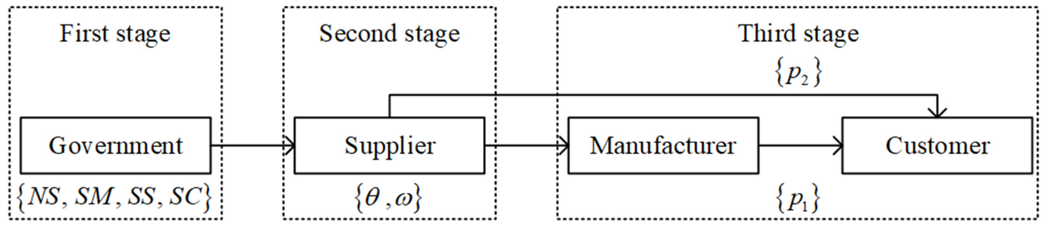
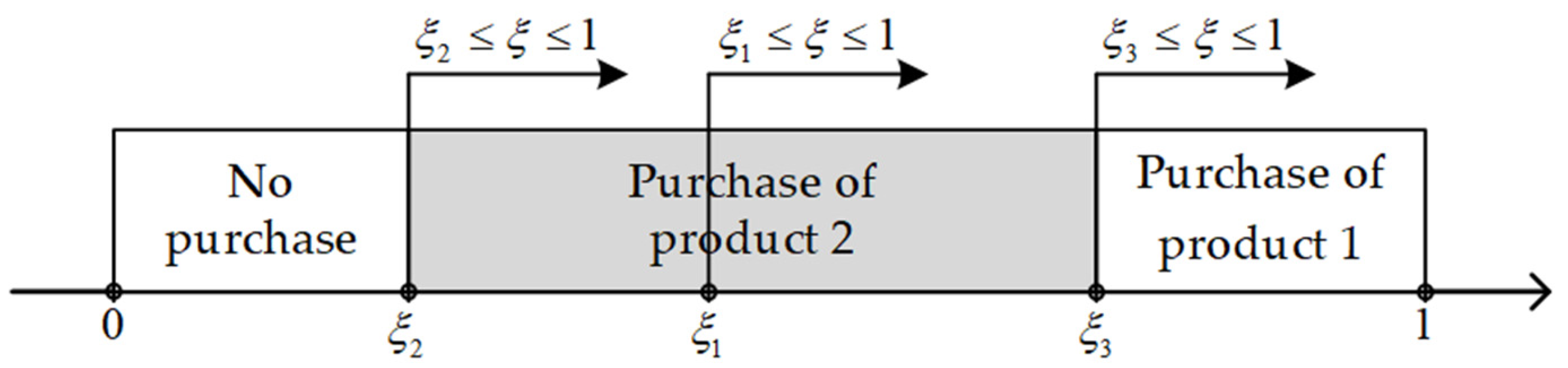
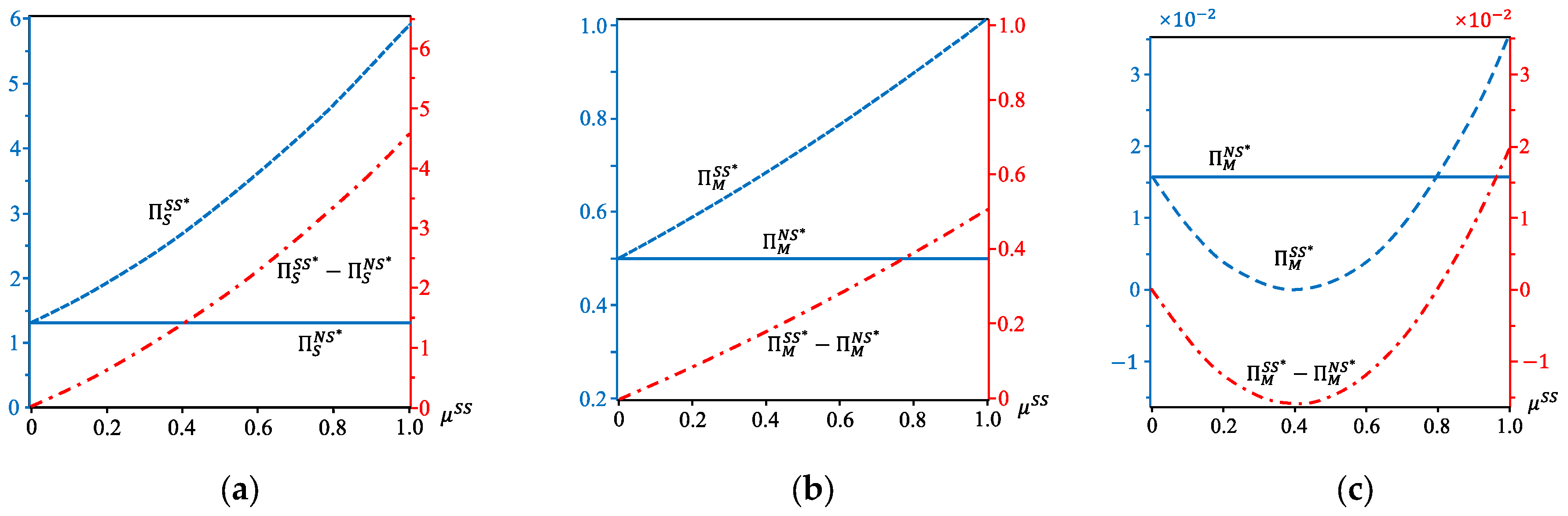
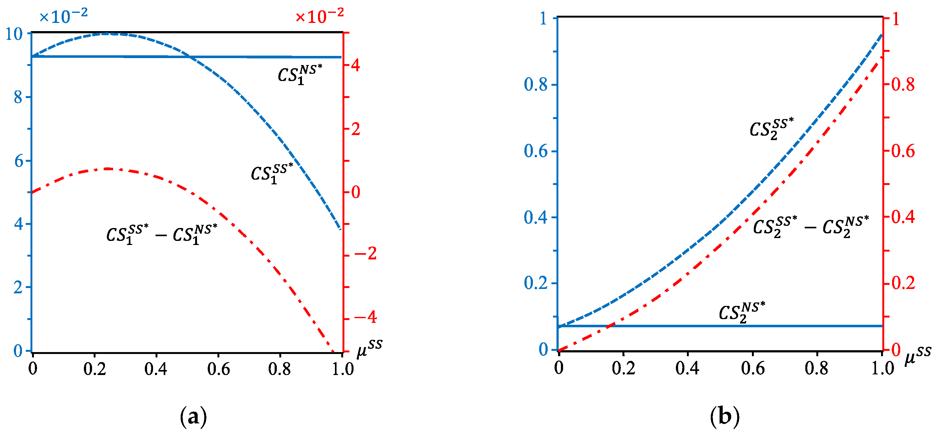
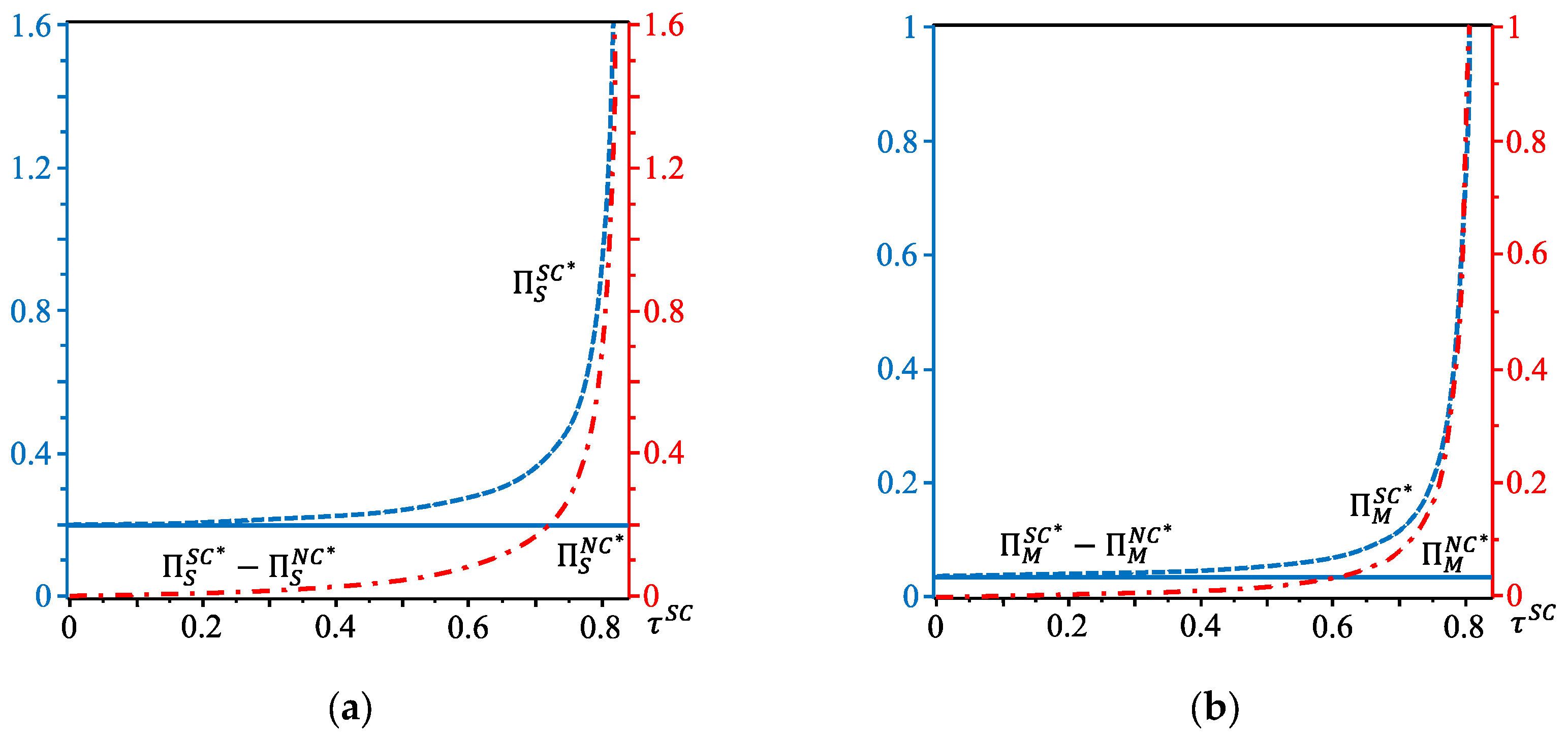
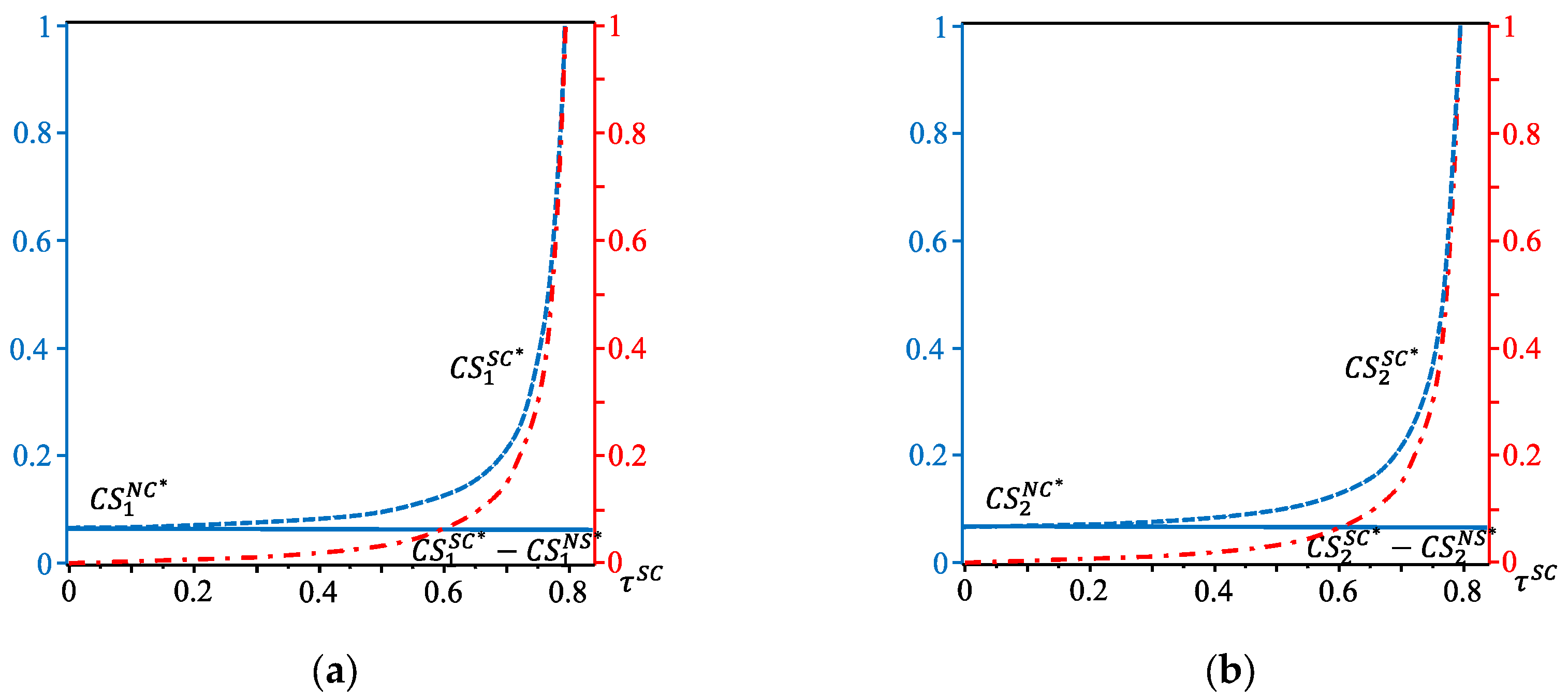
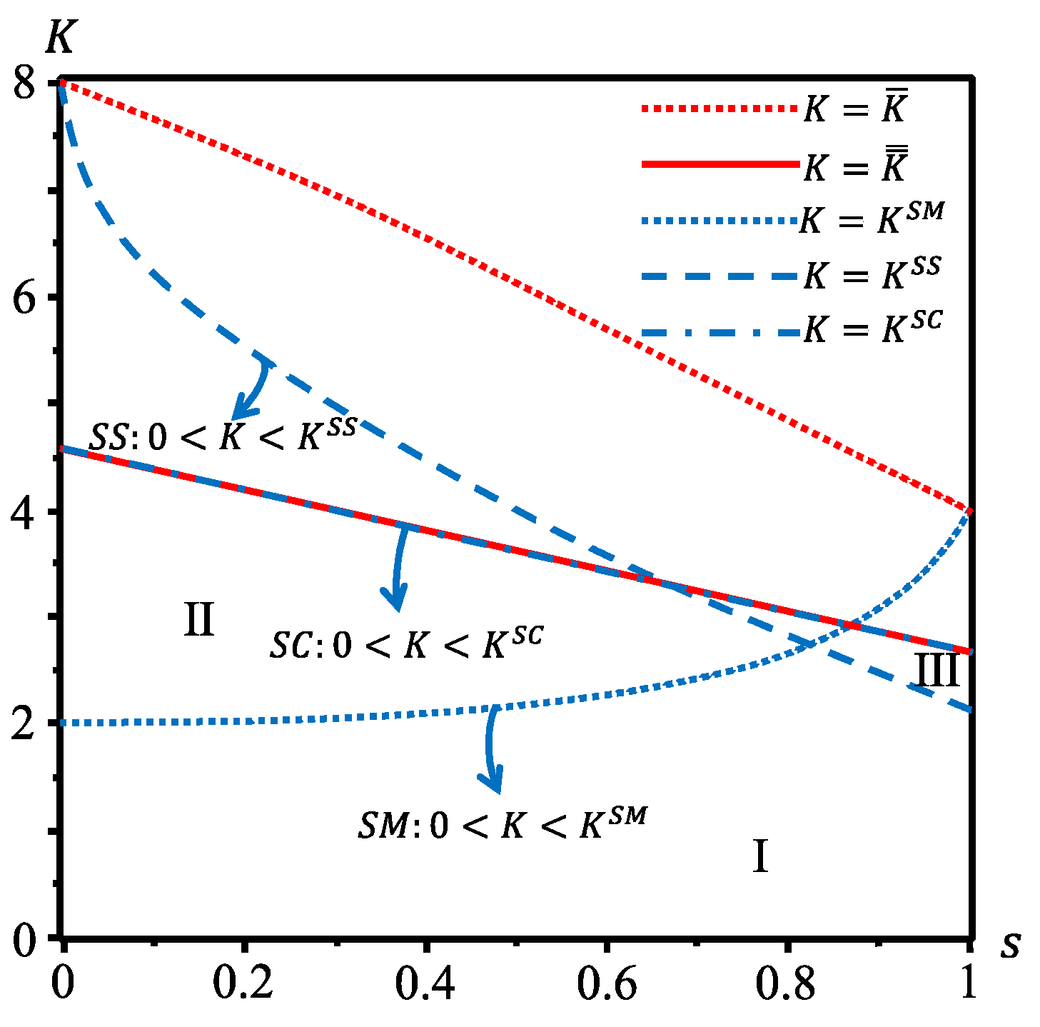
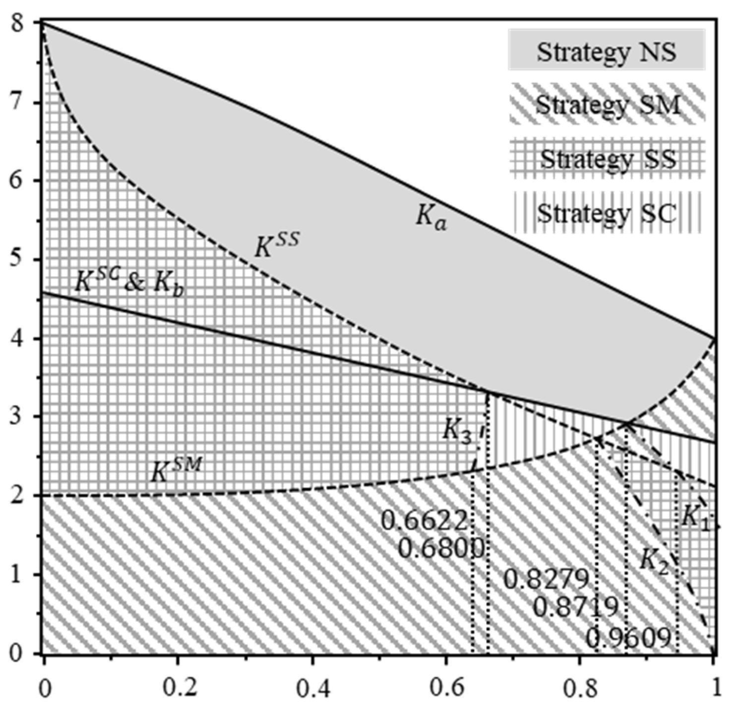
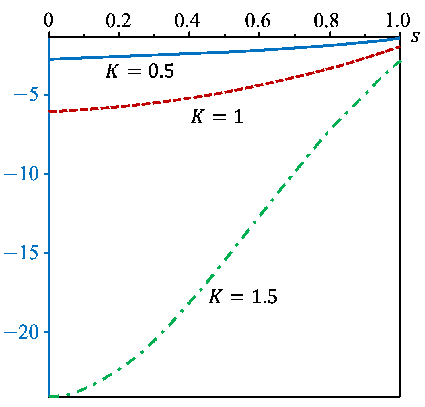
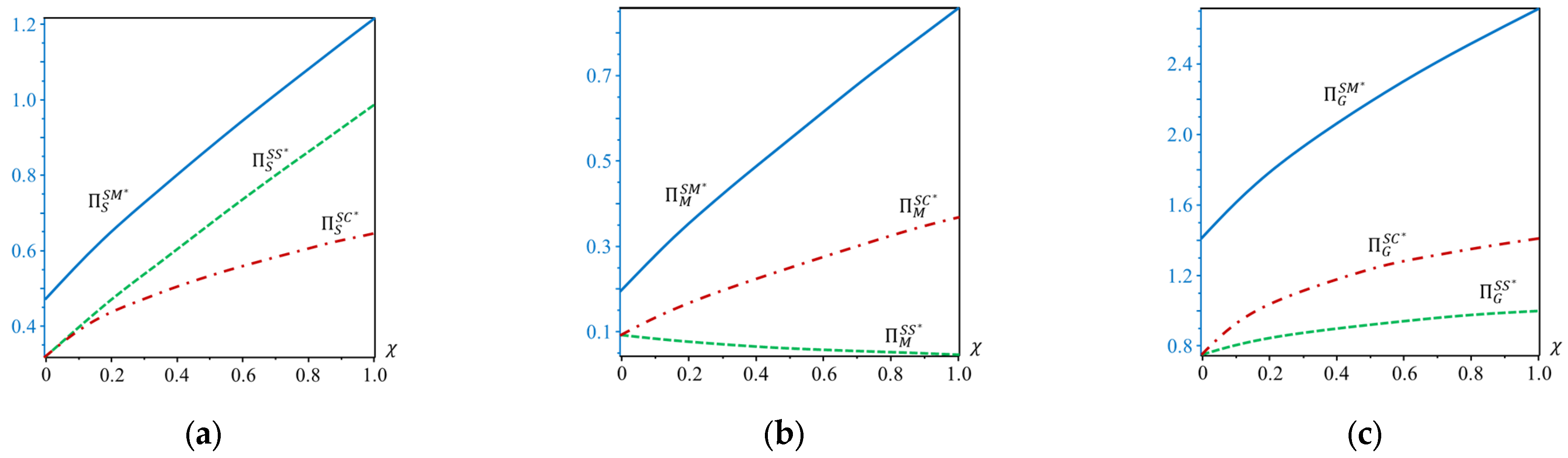