Abstract
For decades, understanding the dynamics of infectious diseases and halting their spread has been a major focus of mathematical modelling and epidemiology. The stochastic SIRS (susceptible–infectious–recovered–susceptible) reaction–diffusion model is a complicated but crucial computational scheme due to the combination of partial immunity and an incidence rate. Considering the randomness of individual interactions and the spread of illnesses via space, this model is a powerful instrument for studying the spread and evolution of infectious diseases in populations with different immunity levels. A stochastic explicit finite difference scheme is proposed for solving stochastic partial differential equations. The scheme is comprised of predictor–corrector stages. The stability and consistency in the mean square sense are also provided. The scheme is applied to diffusive epidemic models with incidence rates and partial immunity. The proposed scheme with space’s second-order central difference formula solves deterministic and stochastic models. The effect of transmission rate and coefficient of partial immunity on susceptible, infected, and recovered people are also deliberated. The deterministic model is also solved by the existing Euler and non-standard finite difference methods, and it is found that the proposed scheme forms better than the existing non-standard finite difference method. Providing insights into disease dynamics, control tactics, and the influence of immunity, the computational framework for the stochastic SIRS reaction–diffusion model with partial immunity and an incidence rate has broad applications in epidemiology. Public health and disease control ultimately benefit from its application to the study and management of infectious illnesses in various settings.
Keywords:
stochastic numerical scheme; stability; consistency; diffusive SIRS model; partial immunity; incidence rate and disease spread MSC:
35R60; 65C30; 65M12
1. Introduction
For the stochastic diffusive epidemic model with partial immunity and an incidence rate, a finite difference approach is a numerical method for solving the partial differential equation (PDE). The PDE describes time- and space-variant population dynamics of the susceptible, infected, and recovered groups. The model’s incidence rate term describes how quickly new infections spread. At the same time, the partial immunity factor considers that not everyone is vulnerable to the disease. The finite difference method transforms the PDE into a set of ODEs, which can then be solved numerically. The spatial domain is grid-divided, and finite difference operators are used to approximate the PDE derivatives. Multiple numerical techniques can then be used to solve the resulting system of ODEs.
The Euler technique is frequently used to resolve the system of ODEs. The Euler method’s simplicity and explicitness may lead to inaccuracies when dealing with enormous time increments. The Crank–Nicolson approach is more precise. However, it is implicit. Compared to the Euler method, the Crank–Nicolson approach is more stable but demands more processing power.
Using a stochastic solver is an alternative method for resolving the system of ODEs. A stochastic solver would consider the unpredictability of the disease’s spread. Diseases with low transmission rates or those whose prevalence is influenced by environmental variables may benefit from this type of modelling.
When simulating the spread of infectious disease, stochastic modelling is a common approach for examining the underlying dynamics of the disease. More so, it has been seen that stochastic models are typically more illuminating than deterministic ones since the latter can only predict one outcome given a particular set of conditions. A stochastic model, on the other hand, forecasts several different possibilities. Using stochastic differential equations, numerous scholars have suggested numerous mathematical models to characterize the dynamics of epidemics in recent years (e.g., Refs. [1,2,3,4]). To obtain more realistic systems of population interactions, authors have inserted temporal delays into such models and explored their dynamical properties (see, for example, Refs. [5,6,7]).
Vaccination has the potential to play a significant role in disease control by reducing the rate of reproduction and, consequently, the number of sick people in an endemic region. It is well established that certain vaccines produce just transitory immunity while others provide lifelong protection. Thus, the time it takes for an individual to develop immunity to an infection or vaccine is considered a delay factor in many published works’ construction of epidemic models (for example, refer to Refs. [8,9,10]). Based on the equivalent deterministic model developed and explored in [11], the authors in [12] devised the stochastic SVIR epidemic model. This was carried out because vaccinations are such an efficient technique for reducing diseases.
It is common knowledge that accurate epidemic modelling relies heavily on accurate incidence rates to explain infectious disease dynamics. Many researchers have advocated nonlinear incidence rates as a more flexible model for dealing with genuine data and a more nuanced approach to analyzing disease transmission than bilinear and standard incidence rates [13].
A universal functional response was recently introduced by Hattaf et al. [14], where are saturation factors assessing the psychological or inhibitory effect. Using this equation, we can extrapolate from the literature a wide variety of incidence rates. If , for instance (see [15]), we obtain the bilinear incidence rate . If , or if , the saturated incidence function is produced (see [16,17]). If , the Beddington–DeAngelis functional response is achieved (see [18,19] for details). If , the Crowley–Martin functional response is found to be .
However, the influence of vaccinations on public health in populations is significantly impacted by the duration of immunity, making it one of the most crucial components of disease and vaccines. Individual immunity to infectious diseases was shown to last anywhere from a few months to a lifetime [20]. For instance, the protection afforded by the varicella [21] and pertussis [22] vaccines against infectious diseases is only brief. Loss of immunological memory and the evolution of the disease are two key reasons why immunity (whether infection-induced or vaccination-induced) diminishes for many infectious disorders [23].
A few researchers have worked on numerical solutions to the epidemic models. While Nowak et al. [24] proposed a deterministic model for the simulation of hepatitis B virus infection, Wang and Wang [25] proposed an alternative model in which the virus moves randomly, and the concentration gradient is assumed to be proportional to the virus’s population flux. Suryanto et al. provided a non-standard FDS for the numerical approximation of the SIR epidemic model with a saturated incidence rate. The scheme results are dynamically consistent with the continuous model [26]. Naik et al. assumed a Crowley–Martin functional response and a Holling type-II treatment rate for the SIR epidemic model. They turned to homotopy analysis for the analytical solutions of the provided model. The authors consider the model’s stability and find it can exist in two distinct states: disease-free and endemic [27].
Physical phenomenon modelling is a fascinating field of study and practice. Partial differential equations (PDEs) are utilized because they accurately describe the underlying physical behavior [28,29,30,31]. There is a lot of research in the field of solving PDEs, and many different methods are used [32,33,34,35,36,37,38]. Forty years ago, it was widely believed that advances in nutrition, pharmaceuticals, and vaccines were largely responsible for the dramatic drop in the human mortality rate that occurred then. Infectious infections have always been a major problem for people and cattle. Traditional epidemic models cannot capture how illnesses behave. As a result, it is crucial to think about epidemic models within a stochastic framework. Therefore, fresh case-specific literature is necessary. The dynamics of stochastic partial differential equations are the subject of many recent investigations. The authors performed in-depth analyses of several physical phenomena using the finite difference scheme [39,40,41]. Macas-Daz et al. [42] studied the stochastic epidemiology model using a non-traditional finite difference approach. The dynamics of a stochastic model of smoking were investigated by Raza et al., who devised a non-standard finite difference to do so [43]. The stochastic fractional epidemic model was numerically approximated by Nauman et al. [44]. The stochastic dengue epidemic model was solved by Raza et al. [45]. Alkhazzan et al. [46] examined and discussed the dynamics of an SVIR epidemic model. The utilization of the fractional order Caputo fractional derivative co-infection illness epidemic model has been examined in previous studies [47,48,49,50]. In chemistry, MiR-17-92 is critical in regulating the Myc/E2F protein. A novel fractional-order delayed Myc/E2F/miR-17-92 network model revealing their relationship is proposed in [51].
There are several potential uses for the computational scheme developed for the stochastic (SIRS) reaction–diffusion model with partial immunity and an incidence rate in epidemiology and other fields of study. Some important information about its uses is as follows:
- Epidemiological Modelling: The primary use of this computational framework is the modelling of infectious disease dynamics in populations. Because it allows researchers to examine the impact of partial immunity on disease transmission and prevalence, it is especially helpful when thinking about diseases with various levels of immunity. This is particularly important in the case of influenza, where immunity can shift from season to season due to strain changes.
- Geographical Spread Analysis: Because this model includes diffusion, it can be used to analyze the geographical spread of diseases. The ability to optimize healthcare resource allocation and implement effective control measures relies on researchers thoroughly understanding how diseases spread across geographic regions.
- Vaccination Strategy: Vaccination techniques can be tested using the model. It is useful for calculating the effects of vaccination rates, waning immunity, and partial immunity on the overall disease burden in a community. Policymakers might use these data as a reference when deciding how to proceed with vaccination drives.
- Public Health Policy Planning: Infectious disease dynamics knowledge is essential for public health policymaking. This model can shed light on how factors like incidence rates and geographic location influence the spread of disease. It is useful for determining how to allocate resources best and implement intervention techniques to reduce disease spread.
- Disease Evolution: By adding partial immunity, the model may also be used to examine how diseases change over time. The immune response to diseases like HIV is complex and changes over time, which is particularly relevant. The model can show how the disease may evolve and how therapies may alter its course.
Suppose you want to simulate the spread of disease. In that case, you can use the finite difference approach or a computational methodology for a stochastic diffusive epidemic model with partial immunity and an incidence rate. This technique can examine how changing certain variables impacts disease transmission and how efficient certain preventative strategies are.
Researchers and public health officials can use the finite difference approach or computational scheme for a stochastic diffusive epidemic model with partial immunity and an incidence rate to better understand and manage disease transmission.
The solutions to the epidemic models can be found by applying analytical and numerical methods. The analytical methods sometimes take more time to converge than numerical methods when applied to nonlinear problems. Different methods exist to handle nonlinear term(s) in differential equations. However, nonlinear terms are linearized using implicit finite difference methods. However, for the explicit methods, linearization is not required. So, linear finite difference schemes are sometimes useful for solving nonlinear differential equations. An iterative method can also be adopted to overcome the deficiency of explicit schemes when applied to problems having Neumann-type boundary conditions. An iterative scheme is also employed in this work to manage such cases. The stopping criteria of the iterative scheme for the deterministic model are also provided, and the iterative will be stopped if this criterion is met. The Wiener process term is approximated by the MATLAB built-in function of using normal distribution with mean zero. So, the MATLAB built-in facility is adopted for solving the stochastic diffusive epidemic model.
Public Health Benefits:
As a powerful tool for comprehending and controlling infectious diseases, the suggested computational framework for the stochastic SIRS reaction–diffusion model with partial immunity and an incidence rate provides substantial advantages to public health. By including an incidence rate and partial immunity, the model provides a more accurate portrayal of disease dynamics in populations with different immunity levels. By taking into account the inherent unpredictability in the interactions between individuals and the distribution of diseases over space, the computational scheme’s stochastic explicit finite difference method helps to model the dynamics of infectious disease transmission and evolution.
An effective strategy for disease control can be developed with the use of the model’s findings. Key parameters impacting disease dynamics can be identified by studying the influence of transmission rates and coefficients of partial immunity on susceptible, infected, and recovered people using the model. With this information, we may better develop public health plans and tailored interventions to reduce the transmission of infectious illnesses in various environments. In the end, public health authorities and lawmakers can make better disease prevention and control decisions because of the computational framework’s extensive use in epidemiology.
Limitations of the Study:
Even though the suggested computational paradigm sheds light on the dynamics of infectious diseases, its limits must be recognized. The mathematical model’s assumptions regarding homogenous mixing and constant parameters, among other simplifications, are restricted. Complex real-world interactions and population-level fluctuations may be beyond the scope of these assumptions.
Furthermore, the model assumes partial immunity, the integrity of which depends on the accessibility of pertinent data and the thoroughness of immunity-related elements taken into account.
Validation of Methods:
It is necessary to validate the stability and consistency of the suggested computational strategy in the mean square sense and apply it to diffusive epidemic models with incidence rates and partial immunity. To further explore the process of validation, the subsequent variables are examined:
Stability: The scheme’s stability is guaranteed by a thorough analysis that considers the predictor–corrector stages. Establishing stability criteria demonstrates that the numerical solution exhibits convergence towards the accurate solution when the discretization parameters progressively decrease.
Consistency: verifying consistency in the mean square sense demonstrates that as the grid spacing decreases, the numerical solution converges to the theoretical solution of the stochastic partial differential equations.
Comparison with existing model: The new technique is evaluated using the existing Euler method and a non-standard finite difference method. The suggested technique is demonstrated to be superior to the existing non-standard finite difference method in solving the deterministic model through the provision of well-defined metrics and performance indicators.
The reliability and correctness of the proposed computational scheme in capturing the dynamics of infectious diseases within the stochastic SIRS reaction–diffusion model framework with partial immunity and an incidence rate are ensured by implementing a complete validation technique.
2. Stochastic Computational Scheme
An explicit two-stage scheme is proposed that can solve stochastic differential equations. Both stages of the scheme are explicit. The scheme consists of a fixed step size. The first stage of the scheme is the Euler–Maruyama method, and the second stage contains parameters that will be found later by comparing Taylor series expansion. For starting the constructing procedure of the scheme, consider the following stochastic partial differential equation:
where is a constant, and represents a Winner process.
The proposed scheme will be constructed for the deterministic model (1). i.e., . Later on, the scheme will be constructed for the stochastic model (1).
The first stage of the scheme is expressed as:
where represents the solutions of Equation (1) computed at grid point and at an arbitrary time level. The solution computed at the first stage should not considered as a final solution at level. Stage (2) can also be considered as the predictor stage. The corrector stage can be expressed as:
The values of parameters and can be determined by considering the Taylor series expansion of as:
By substituting Equation (4) into Equation (3), the following is obtained:
By using (2) into Equation (5):
Equating coefficients of and on both sides of Equation (6) yields:
Solving Equation (7), the values of and can be expressed as:
The semi-discretization for stochastic Equation (1) is given by:
and
where and will be chosen from Equation (8) and .
Letting in Equation (1), the fully discretized equations are:
and
3. Stability Analysis
The stability analysis of the proposed scheme for stochastic parabolic linear equations will be performed by applying Fourier series analysis. The analysis provides the conditions on step size and involved parameters. The stability analysis assumes the dependent variable by the component of the Fourier series. The transformations are given as:
where .
It yields by substituting some of the transformations from Equation (13) into the first stage of the proposed scheme (11).
Dividing both sides of Equation (14) by yields:
where .
Using trigonometric identities yields:
Similarly, upon substituting some of the transformations from Equation (13) into the second stage of the proposed scheme (12), it gives:
Dividing both sides of Equation (16) by yields:
Using Equation (15) in Equation (17) produces:
The amplification factor for the scheme is given as:
Applying the expected value on the square of amplitudes of the two consecutive Fourier components of the solution of the differential equations using the proposed scheme and also using the inequality give the stability condition for the proposed stochastic scheme as:
If
and let
Then, inequality (20) can be expressed as:
Therefore, the proposed stochastic numerical scheme is conditionally stable.
Theorem 1.
The proposed stochastic numerical scheme (11)–(12) is consistent in the mean square sense.
Proof.
Let be the smooth function:
where .
The following equations can be obtained from Equations (22) and (23):
Equation (24) can be rewritten as:
Now, the following result is used:
where is the initial time.
By using the result (26) in (25), the following inequality can be obtained:
Thus, implementation of limits when and then results in:
Therefore, the proposed stochastic numerical scheme is consistent in the mean square sense. □
4. Diffusive Stochastic Epidemic Model
Let and represent the densities of susceptible, infectious, and recovered people at location and time . Letting represent the transmission rate and denote the natural mortality of people, is used for mortality caused by the disease, denotes the rate of losing of immunity, denotes the birth rate of susceptible people, represents the recovery rate, and these functions are positive Holder continuous functions. By following [52] for the deterministic model, the stochastic SIRS model is expressed as:
Subject to the boundary conditions:
and initial conditions are given as:
For and , the disease-free equilibrium points can be determined from the following equations:
By solving Equations (34)–(36), the disease-free equilibrium points are found as:
Theorem 2.
The system of Equations (29)–(31) with and is locally stable if .
Proof.
The Jacobian of the system (29)–(31) with and is given as:
The Jacobian at the disease-free equilibrium point is given by:
The Eigenvalue of is found to be:
Since and are negative, and will be negative if:
it is implied that:
□
5. Discussions
A stochastic finite difference method is proposed, which is an explicit scheme. The scheme can be applied to discretize time variables in the considered stochastic parabolic equations. The second-order central difference formulas discretize the space terms since the considered diffusive epidemic model consists of the second-order spatial derivatives. The scheme is conditionally stable, and it is conditionally convergent. The scheme can be used for both classical and stochastic parabolic equations. The stability condition of the scheme depends upon both the time and space step sizes and the contained parameters in the epidemic diffusive model. For the adopted model, the boundary conditions are Neumann type. So, to handle these boundary conditions using the finite difference explicit scheme, an additional iterative scheme is also employed. The iterative scheme requires an initial guess to start the solution procedure. It also requires a stopping criterion for breaking the loop over the iterations. The outer loop is employed for using the iterative scheme that will be stopped if the maximum of norms of solutions computed on two consecutive iterations will be less than some tolerance. The iterative scheme will be stopped if the solution satisfies the mentioned criterion. Otherwise, it will continue to find the solution over the new iteration. So, the convergence of the solution depends on the employed numerical schemes for discretizing the stochastic partial differential equations and stopping or converging the criteria of the iterative scheme.
Given the abundance of mathematical models about epidemic diseases documented in the literature, employing an approximate analytical or numerical scheme to solve even the most complex ones is necessary. A numerical scheme for solving deterministic and stochastic models is proposed in this work. Additionally, existing numerical schemes for deterministic cases are contrasted to the scheme. The scheme under consideration is capable of solving both deterministic and stochastic models. The Euler–Maruyama technique is available as a method for solving stochastic differential equations. The method applies stochastic models to the classical forwards Euler method for deterministic models. If the coefficient of the Weiner process term remains constant, the method precisely integrates it. However, it approximates the integral of the Weiner process term with respect to the variable coefficient. The proposed methodology yields a more precise solution for deterministic models than the Euler method. Approximating the integral of the stochastic component of the differential equation is the function of the stochastic component of the scheme.
6. Results
There exist numerical schemes for finding solutions to epidemic models and providing a guarantee for obtaining positive solutions. Among these schemes, the non-standard finite difference method (NSFD) can be used to solve epidemic models and guarantee the positivity of the solution. Among the existing NSFD methods, one provides an unconditionally stable solution and gives surety for the positive solution. In this work, a comparison of the proposed numerical scheme is made with the existing NSFD method. Figure 1 compares the stochastic and deterministic solutions using the proposed scheme. Figure 2, Figure 3 and Figure 4 show this comparison, and the first-order forward Euler method obtains the solution. Due to the lack of first-order accuracy of the NSFD, the obtained solution deviates slightly from the first- or second-order solutions. The first-order solution is obtained by employing the forward Euler method, and the second-order solution is obtained by the proposed scheme for the deterministic model. This deficiency in existing finite difference has also been proved in [53] for the diffusive models. Since the solutions to an epidemic remain positive for some chosen values of parameters, any numerical scheme can be considered for those cases. Therefore, the proposed scheme and first-order Euler methods are also employed for the epidemic model. Figure 5 shows the effect of the transmission rate parameter on the susceptible people. The susceptible people grow by rising transmission rate parameters. The effect of the transmission rate parameter on infected people can be seen in Figure 6. The infected people grow as the transmission rate parameter enhances. The effect of the transmission rate parameter on recovered people can be seen in Figure 7. The recovered people are also grown by rising transmission rate parameters. Since recovered people become susceptible, when recovered people grow, the susceptible people also grow. The number of infected people increases because susceptibility converts to infection by rising transmission rate parameters. The effect of the coefficient of partial immunity on susceptible individuals is shown in Figure 8. The susceptible people decay by the rising coefficient of the partial immunity parameter. Figure 9 and Figure 10 show the effect of the coefficient of partial immunity on infected and recovered people. The infected people decay, and the recovered people grow by enhancing the coefficient of partial immunity. The coefficient of partial immunity produces growth in the body’s immune system, leading to decay in infected people and growth in recovered people. Figure 11, Figure 12 and Figure 13 show the contour plots for susceptible, infected, and recovered people for the deterministic model. The variation in both space coordinates can be seen in these contour plots. The mesh plots underneath the contours are also displayed in Figure 14, Figure 15 and Figure 16 for the stochastic model. The effect of the Wiener process term can be seen in the mesh underneath the contour plots. The large coefficient of the Wiener process term gives more oscillation-type solutions than those with a small coefficient of Weiner process terms.
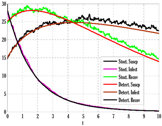
Figure 1.
Comparison of stochastic and deterministic solutions of the considered model using .
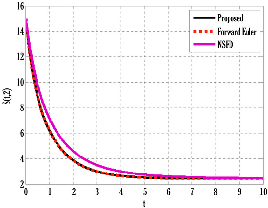
Figure 2.
Comparison of proposed, Euler, and NSFD methods for susceptible people in the deterministic model using .
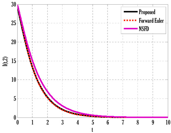
Figure 3.
Comparison of proposed, Euler, and NSFD methods for infected people in the deterministic model using .
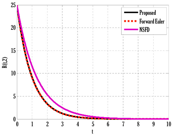
Figure 4.
Comparison of proposed, Euler, and NSFD methods for recovered people in the deterministic model using .
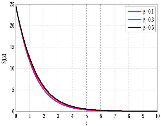
Figure 5.
Effect of transmission rate on susceptible people in the deterministic model using .
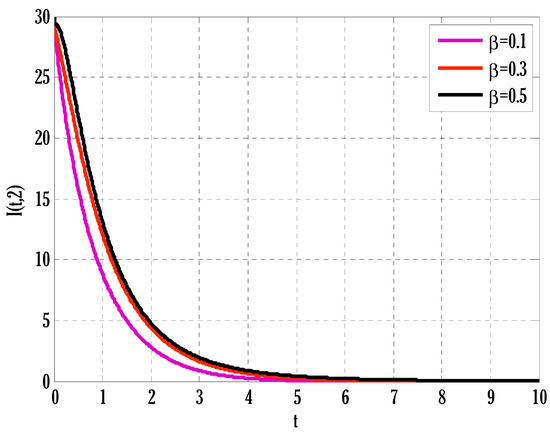
Figure 6.
Effect of transmission rate on infected people in the deterministic model using .
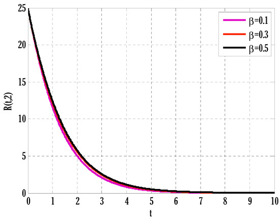
Figure 7.
Effect of transmission rate on recovered people in the deterministic model using .
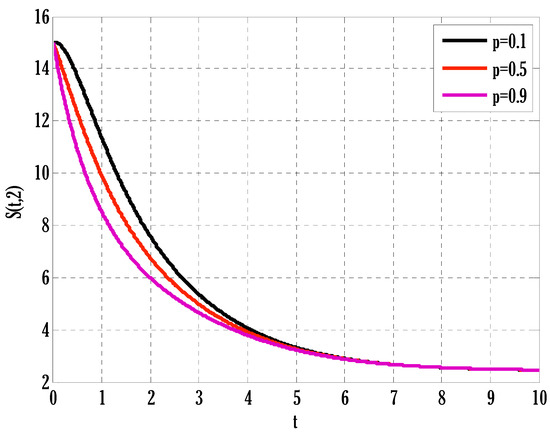
Figure 8.
Effect of coefficient of partial immunity on susceptible people in the deterministic model using .
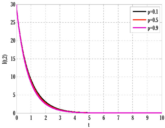
Figure 9.
Effect of coefficient of partial immunity on infected people in the deterministic model using .
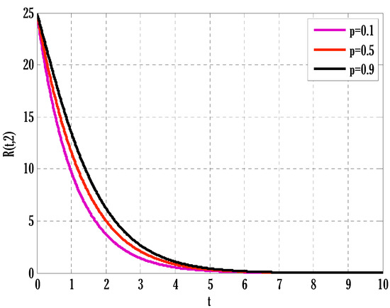
Figure 10.
Effect of coefficient of partial immunity on recovered people in the deterministic model using .
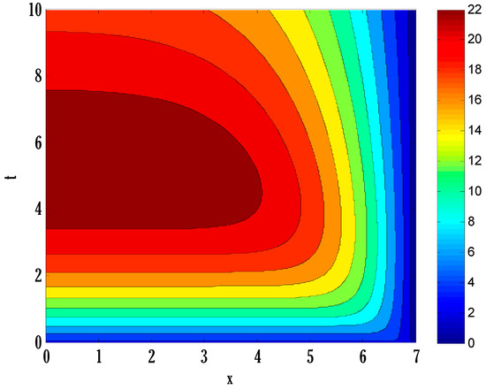
Figure 11.
Contour plot on susceptible people in the deterministic model using .
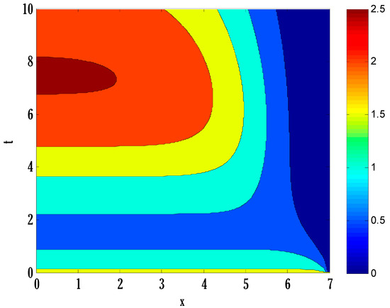
Figure 12.
Contour plot on infected people in the deterministic model using .
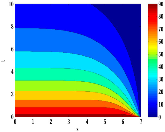
Figure 13.
Contour plot on recovered people in the deterministic model using .
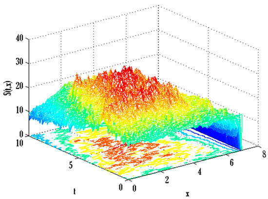
Figure 14.
Mesh plot underneath contours for susceptible people of the stochastic model using .
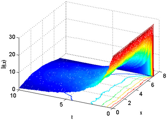
Figure 15.
Mesh plot underneath contours for infected people of the stochastic model using .
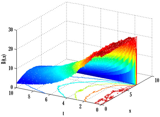
Figure 16.
Mesh plot underneath contours for recovered people of the stochastic model using .
7. Conclusions
A computational scheme has been proposed for solving the stochastic diffusive SIRS model with an incidence rate and partial immunity. An additional iterative scheme has also been employed for handling Neumann-type boundary conditions applied on each domain end. So, a stopping criterion was also set up to stop the iterative procedure for the deterministic model. The computational framework utilized for the stochastic SIRS reaction–diffusion model with partial immunity and an incidence rate holds significant potential and adaptability within epidemiology and mathematical modelling. It has wide-ranging uses and can improve our understanding of infectious disease dynamics and help us create better prevention and treatment methods. Due to its ability to account for factors including partial immunity, regional diffusion, and changing incidence rates, this model is invaluable for public health planning and disease management. This computational technique adds to our understanding of infectious diseases in various populations and geographical locations by examining the complex relationship between immunity, spatial spread, and disease transmission. In the face of new infectious diseases and endemic pathogens, it is crucial to assess immunization tactics, research disease evolution, and forecast future trends. Because of its stochastic nature, the model more accurately represents epidemiological processes, which is important because of the inherent uncertainty in disease transmission. This is of great use when the spread of a disease is heavily influenced by chance and the activities of individuals. This method links theoretical epidemiological studies and real-world public health policymaking. The concluding points can be expressed as:
- Comparison showed that the proposed scheme was more accurate than the existing NSFD scheme for the deterministic model.
- Susceptible, infected, and recovered people were seen to grow by enhancing transmission parameters.
- Infected and recovered people were also grown by raising the coefficient of partial immunity.
- The proposed scheme performed better than the existing non-standard finite difference method in order of accuracy.
The stochastic SIRS reaction–diffusion model with partial immunity and an incidence rate is useful for researchers, politicians, and medical professionals in a world where infectious illnesses threaten public health systems. Using it, we may better manage infectious disease outbreaks, distribute scarce resources, and prepare for emergencies, all of which improve public health and lessen these crises’ toll on the world’s population. Upon the conclusion of this project, it is possible to propose further applications for the existing strategy [54,55,56]. This model will continue to be at the forefront of attempts to address the ever-changing environment of infectious illnesses as research in this field develops.
Author Contributions
Conceptualization, methodology, and analysis, A.S.B.; funding acquisition, A.S.B.; investigation, Y.N.; methodology, Y.N.; visualization, M.S.A.; writing—review and editing, M.S.A.; resources, K.A.; supervision, K.A.; data curation, M.A.A.; formal analysis, M.A.A. All authors have read and agreed to the published version of the manuscript.
Funding
This work was supported and funded by the Deanship of Scientific Research at Imam Mohammad Ibn Saud Islamic University (IMSIU) (grant number IMSIU-RG23014).
Data Availability Statement
The manuscript includes all required data and implementing information.
Acknowledgments
This research was supported by the Deanship of Scientific Research, Imam Mohammad Ibn Saud Islamic University (IMSIU), Saudi Arabia, Grant No. (IMSIU-RG23014).
Conflicts of Interest
The authors declare no conflict of interest to report regarding the present study.
References
- Adnani, J.; Hattaf, K.; Yousfi, N. Stability Analysis of a Stochastic SIR Epidemic Model with Specific Nonlinear Incidence Rate. Int. J. Stoch. Anal. 2013, 2013, 431257. [Google Scholar] [CrossRef]
- Jehad, A.; Ghada, A.; Shah, H.; Elissa, N.; Hasib, K. Stochastic dynamics of influenza infection: Qualitative analysis and numerical results. Math. Biosci. Eng. 2022, 19, 10316–10331. [Google Scholar]
- Shah, H.; Elissa, N.; Hasib, K.; Haseena, G.; Sina, E.; Shahram, R.; Mohammed, K. On the Stochastic Modeling of COVID-19 under the Environmental White Noise. J. Funct. Spaces 2022, 2022, 4320865. [Google Scholar]
- Miaomiao, G.; Daqing, J.; Tasawar, H. Stationary distribution and periodic solution of stochasticchemostat models with single-species growthon two nutrients. Int. J. Biomath. 2019, 12, 1950063. [Google Scholar]
- Liu, Q.; Jiang, D.; Shi, N.; Hayat, T.; Alsaedi, A. Asymptotic behavior of a stochastic delayed SEIR epidemic model with nonlinear incidence. Phys. A 2016, 462, 870–882. [Google Scholar] [CrossRef]
- Tailei, Z.; Zhidong, T. Global asymptotic stability of a delayed SEIRS epidemic model with saturation incidence. Chaos Solitons Fractals 2008, 37, 1456–1468. [Google Scholar]
- Rui, X.; Zhien, M. Global stability of a SIR epidemic model with nonlinear incidence rate and time delay. Nonlinear Anal. Real World Appl. 2009, 10, 3175–3189. [Google Scholar]
- Hattaf, K.; Mahrouf, M.; Adnani, J.; Yousfi, N. Qualitative analysis of a stochastic epidemic model with specific functional response and temporary immunity. Phys. A 2018, 490, 591–600. [Google Scholar] [CrossRef]
- Pitchaimani, M.; Brasanna, D.M. Stochastic dynamical probes in a triple delayed SICR model with general incidence rate and immunization strategies. Chaos Solitons Fractals 2021, 143, 110540. [Google Scholar]
- Xu, C.; Li, X. The threshold of a stochastic delayed SIRS epidemic model with temporary immunity and vaccination. Chaos Solitons Fractals 2018, 111, 227–234. [Google Scholar] [CrossRef]
- Xianning, L.; Yasuhiro, T.; Shingo, I. SVIR epidemic models with vaccination strategies. J. Theoret. Biol. 2008, 253, 1–11. [Google Scholar]
- Zhang, X.; Jiang, D.; Hayat, T.; Ahmad, B. Dynamical behavior of a stochastic SVIR epidemic model with vaccination. Phys. A 2017, 483, 94–108. [Google Scholar] [CrossRef]
- Li, F.; Zhang, S.Q.; Meng, X.Z. Dynamics analysis and numerical simulations of a delayed stochastic epidemic model subject to a general response function. Comput. Appl. Math. 2019, 38, 95. [Google Scholar] [CrossRef]
- Hattaf, K.; Yousfi, N.; Tridane, A. Stability analysis of a virus dynamics model with general incidence rate and two delays. Appl. Math. Comput. 2013, 221, 514–521. [Google Scholar] [CrossRef]
- Wang, J.; Zhang, J.; Jin, Z. Analysis of an SIR model with bilinear incidence rate. Nonlinear Anal. Real World Appl. 2010, 11, 2390–2402. [Google Scholar] [CrossRef]
- Liu, X.; Yang, L. Stability analysis of an SEIQV epidemic model with saturated incidence rate. Nonlinear Anal. Real World Appl. 2012, 13, 2671–2679. [Google Scholar] [CrossRef]
- Zhao, Y.; Jiang, D. The threshold of a stochastic SIRS epidemic model with saturated incidence. Appl. Math. Lett. 2014, 34, 90–93. [Google Scholar] [CrossRef]
- Cantrell, R.; Cosner, C. On the dynamics of predator-prey models with the Beddington–DeAngelis functional response. J. Math. Anal. Appl. 2001, 257, 206–222. [Google Scholar] [CrossRef]
- Zhou, X.; Cui, J. Global stability of the viral dynamics with Crowley–Martin functional response. Bull. Korean Math. Soc. 2011, 48, 555–574. [Google Scholar] [CrossRef]
- Anderson, R.; Garnett, G. Low-efficacy HIV vaccines: Potential for community-based intervention programmes. Lancet 1996, 348, 1010–1013. [Google Scholar] [CrossRef]
- Chaves, S.; Gargiullo, P.; Zhang, J.; Civen, R.; Guris, D.; Mascola, L.; Seward, J. Loss of vaccine-induced immunity to varicella over time. N. Engl. J. Med. 2007, 356, 1121–1129. [Google Scholar] [CrossRef] [PubMed]
- Wendelboe, A.; Van Rie, A.; Salmaso, S.; Englund, J. Duration of immunity against pertussis after natural infection or vaccination. Pediatr. Infect. Dis. J. 2005, 24, 58–61. [Google Scholar] [CrossRef] [PubMed]
- Craig, M.P. An evolutionary epidemiological mechanism, with applications to type a influenza. Theor. Popul. Biol. 1987, 31, 422–452. [Google Scholar]
- Nowak, M.A.; Bonhoeffer, S.; Hill, A.M.; Boehme, R.; Thomas, H.C.; McDade, H. Viral dynamics in hepatitis B virus infection. Proc. Natl. Acad. Sci. USA 1996, 93, 4398–4402. [Google Scholar] [CrossRef]
- Wang, K.; Wang, W. Propagation of HBV with spatial dependence. Math. Biosci. 2007, 210, 78–95. [Google Scholar] [CrossRef] [PubMed]
- Suryanto, A.; Darti, I. On the non-standard numerical discretization of SIR epidemic model with a saturated incidence rate and vaccination. AIMS Math. 2021, 6, 141–155. [Google Scholar] [CrossRef]
- Naik, P.A.; Zu, J.; Ghoreishi, M. Stability analysis and approximate solution of SIR epidemic model with Crowley–Martin type functional response and holling type-II treatment rate by using homotopy analysis method. J. Appl. Anal. Comput. 2020, 10, 1482–1515. [Google Scholar]
- Ahmad, I.; Khan, M.N.; Inc, M.; Ahmad, H.; Nisar, K.S. Numerical simulation of simulate an anomalous solute transport model via local meshless method. Alex. Eng. J. 2020, 59, 2827–2838. [Google Scholar] [CrossRef]
- Ahmad, H.; Akgül, A.; Khan, T.A.; Stanimirovic, P.S.; Chu, Y.M. New perspective on the conventional solutions of the nonlinear time-fractional partial differential equations. Complexity 2020, 2020, 8829017. [Google Scholar] [CrossRef]
- Ahmad, H.; Khan, T.A.; Stanimirovic, P.S.; Ahmad, I. Modified variational iteration technique for the numerical? solution of fifth order KdV-type equations. J. Appl. Comput. Mech. 2020, 6, 1220–1227. [Google Scholar]
- Ahmad, H.; Seadawy, A.R.; Khana, T.A. Modified variational iteration algorithm to find approximate solutions of nonlinear Parabolic equation. Math. Comput. Simul. 2020, 177, 13–23. [Google Scholar] [CrossRef]
- Ahmad, I.; Ahmad, H.; Inc, M.; Yao, S.W.; Almohsen, B. Application of local meshless method for the solution of two term time fractional-order multi-dimensional PDE arising in heat and mass transfer. Therm. Sci. 2020, 24 (Suppl. S1), 95–105. [Google Scholar] [CrossRef]
- Inc, M.; Khan, M.N.; Ahmad, I.; Yao, S.W.; Ahmad, H.; Thounthong, P. Analysing time-fractional exotic options via efficient local meshless method. Results Phys. 2020, 19, 103385. [Google Scholar] [CrossRef]
- Khan, M.N.; Ahmad, I.; Ahmad, H. A Radial Basis Function Collocation Method for Space-dependent? Inverse Heat Problems. J. Appl. Comput. Mech. 2020. Available online: https://jacm.scu.ac.ir/article_15512_e7b25d7b217ff1267e45fc596fbfa54b.pdf (accessed on 22 November 2023).
- Shah, N.A.; Ahmad, I.; Bazighifan, O.; Abouelregal, A.E.; Ahmad, H. Multistage optimal homotopy asymptotic method for the nonlinear Riccati ordinary differential equation in nonlinear physics. Appl. Math. 2020, 14, 1009–1016. [Google Scholar]
- Wang, F.; Ali, S.N.; Ahmad, I.; Ahmad, H.; Alam, K.M.; Thounthong, P. Solution of Burgers’ equation appears in fluid mechanics by multistage optimal homotopy asymptotic method. Therm. Sci. 2022, 26 1 Pt B, 815–821. [Google Scholar] [CrossRef]
- Liu, X.; Ahsan, M.; Ahmad, M.; Nisar, M.; Liu, X.; Ahmad, I.; Ahmad, H. Applications of Haar wavelet-finite difference hybrid method and its convergence for hyperbolic nonlinear Schrö dinger equation with energy and mass conversion. Energies 2021, 14, 7831. [Google Scholar] [CrossRef]
- Ahsan, M.; Lin, S.; Ahmad, M.; Nisar, M.; Ahmad, I.; Ahmed, H.; Liu, X. A Haar wavelet-based scheme for finding the control parameter in nonlinear inverse heat conduction equation. Open Phys. 2021, 19, 722–734. [Google Scholar] [CrossRef]
- Yasin, M.W.; Ahmed, N.; Iqbal, M.S.; Rafiq, M.; Raza, A.; Akgül, A. Reliable numerical analysis for stochastic reaction–diffusion system. Phys. Scr. 2022, 98, 015209. [Google Scholar] [CrossRef]
- Wang, X.; Yasin, M.W.; Ahmed, N.; Rafiq, M.; Abbas, M. Numerical approximations of stochastic Gray–Scott model with two novel schemes. AIMS Math. 2023, 8, 5124–5147. [Google Scholar] [CrossRef]
- Yasin, M.W.; Ahmed, N.; Iqbal, M.S.; Raza, A.; Rafiq, M.; Eldin, E.M.T.; Khan, I. Spatio-temporal numerical modeling of stochastic predator–prey model. Sci. Rep. 2023, 13, 1990. [Google Scholar] [CrossRef] [PubMed]
- Macías-Díaz, J.E.; Raza, A.; Ahmed, N.; Rafiq, M. Analysis of a non-standard computer method to simulate a nonlinear stochastic epidemiological model of coronavirus-like diseases. Comput. Methods Prog. Biomed. 2021, 204, 106054. [Google Scholar] [CrossRef] [PubMed]
- Raza, A.; Rafiq, M.; Ahmed, N.; Khan, I.; Nisar, K.S.; Iqbal, Z. A structure preserving numerical method for solution of stochastic epidemic model of smoking dynamics. Comput. Mater. Contin. 2020, 65, 263–278. [Google Scholar] [CrossRef]
- Ahmed, N.; Macías-Díaz, J.E.; Raza, A.; Baleanu, D.; Rafiq, M.; Iqbal, Z.; Ahmad, M.O. Design analysis and comparison of a non-standard computational method for the solution of a general stochastic fractional epidemic model. Axioms 2021, 11, 10. [Google Scholar] [CrossRef]
- Raza, A.; Arif, M.S.; Rafiq, M. A reliable numerical analysis for stochastic dengue epidemic model with incubation period of virus. Adv. Differ. Equ. 2019, 2019, 32. [Google Scholar] [CrossRef]
- Alkhazzan, A.; Wang, J.; Nie, Y.; Hattaf, K. A new stochastic split-step θ-nonstandard finite difference method for the developed SVIR epidemic model with temporary immunities and general incidence rates. Vaccines 2022, 10, 1682. [Google Scholar] [CrossRef]
- Ali, A.; Alshammari, F.S.; Islam, S.; Khan, M.A.; Ullah, S. Modeling and analysis of the dynamics of novel coronavirus (COVID-19) with Caputo fractional derivative. Results Phys. 2021, 20, 103669. [Google Scholar] [CrossRef]
- Ali, A.; Islam, S.; Rasheed, S.; Allehiany, F.; Baili, J.; Khan, M.A.; Ahmad, H. Dynamics of a fractional order Zika virus model with mutant. Alex. Eng. J. 2022, 61, 4821–4836. [Google Scholar] [CrossRef]
- Aba Oud, M.A.; Ali, A.; Alrabaiah, H.; Ullah, S.; Khan, M.A.; Islam, S. A fractional order mathematical model for COVID-19 dynamics with quarantine, isolation, and environmental viral load. Adv. Differ. Equ. 2021, 2021, 106. [Google Scholar] [CrossRef]
- Ali, A.; Ullah, S.; Khan, M.A. The impact of vaccination on the modeling of COVID-19 dynamics: A fractional order model. Nonlinear Dyn. 2022, 110, 3921–3940. [Google Scholar] [CrossRef]
- Li, P.; Peng, X.; Xu, C.; Han, L.; Shi, S. Novel extended mixed controller design for bifurcation control of fractional-order Myc/E2F/miR-17-92 network model concerning delay. Math. Methods Appl. Sci. 2023, 46, 18878–18898. [Google Scholar] [CrossRef]
- Wang, J.; Teng, Z.; Dai, B. Qualitative analysis of a reaction-diffusion SIRS epidemic model with nonlinear incidence rate and partial immunity. Infect. Dis. Model. 2023, 8, 881e911. [Google Scholar] [CrossRef] [PubMed]
- Pasha, S.A.; Nawaz, Y.; Arif, M.S. On the non-standard finite difference method for reaction–diffusion models. Chaos Solitons Fractals 2023, 166, 112929. [Google Scholar] [CrossRef]
- Arif, M.S.; Abodayeh, K.; Nawaz, Y. Construction of a Computational Scheme for the Fuzzy HIV/AIDS Epidemic Model with a Nonlinear Saturated Incidence Rate; Tech Science Press: Norwood, MA, USA, 2023. [Google Scholar] [CrossRef]
- Arif, M.S.; Abodayeh, K.; Nawaz, Y. A Reliable Computational Scheme for Stochastic Reaction–Diffusion Nonlinear Chemical Model. Axioms 2023, 12, 460. [Google Scholar] [CrossRef]
- Nawaz, Y.; Arif, M.S.; Bibi, K.A.A.M. Finite Difference Schemes for Time-Dependent Convection q-Diffusion Problem. AIMS Math. 2022, 7, 16407–16421. [Google Scholar] [CrossRef]
Disclaimer/Publisher’s Note: The statements, opinions and data contained in all publications are solely those of the individual author(s) and contributor(s) and not of MDPI and/or the editor(s). MDPI and/or the editor(s) disclaim responsibility for any injury to people or property resulting from any ideas, methods, instructions or products referred to in the content. |
© 2023 by the authors. Licensee MDPI, Basel, Switzerland. This article is an open access article distributed under the terms and conditions of the Creative Commons Attribution (CC BY) license (https://creativecommons.org/licenses/by/4.0/).