

A Coupled Simulated Annealing and Particle Swarm Optimization Reliability-Based Design Optimization Strategy under Hybrid Uncertainties
 and
and
Abstract
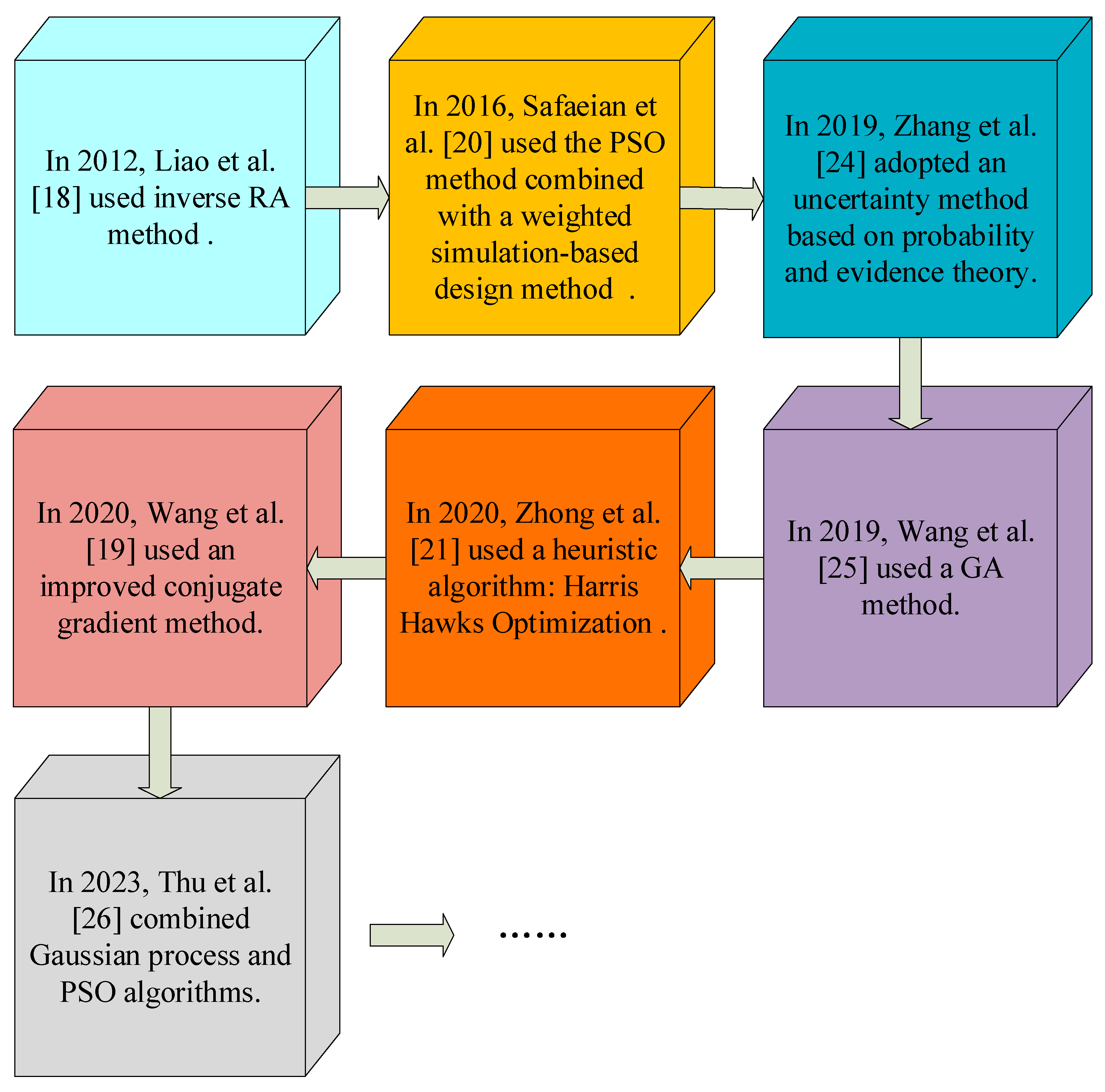
:1. Introduction
2. Two Algorithms for Optimizing the Problem
2.1. Particle Swarm Optimization
2.1.1. Definition of Particle Swarm Optimization
2.1.2. Optimization of PSO Algorithm
2.2. Simulated Annealing Algorithm
2.2.1. Definition of Simulated Annealing Algorithm
2.2.2. Simulated Annealing Algorithm
- (1)
- When the objective function corresponding to the new solution is less than the objective function value of the current solution, it will accept the new solution. That is, the probability of accepting the new solution is 1;
- (2)
- When the corresponding objective function of the new solution is greater than the objective function value of the current solution, the new solution will be accepted with a certain probability. When other variables are certain, the more the value of the objective function corresponding to the new solution exceeds the value of the objective function of the current solution, the smaller the probability of accepting the new solution.
- Step 1: Set the initial temperature ; The initial solution is generated randomly and the objective function is calculated;
- Step 2: Make , ;
- Step 3: Make random perturbation to the current solution , generate a new solution in its field, and calculate its corresponding function value . Meanwhile, judge whether to accept the new solution according to the Metropolis criterion above;
- Step 4: At temperature , iterate the disturbance and acceptance process for times;
- Step 5: Determine whether the terminal temperature is reached. If so, terminate; otherwise, return to step 2.
3. The Combination of Intelligent Algorithms
3.1. First-Order Reliability Method
3.1.1. First-Order Reliability Method
3.1.2. Reliability Index Method
3.1.3. Performance Measure Approach
3.1.4. Reliability Analysis Method Considering Stochastic and Interval Uncertainties
3.1.5. Method of Solving MPP Points by Improving PSO
- Step 1: Set the initial conditions for searching MPP points, including the limit state function , the probability distribution function of the design variable (a normal distribution with mean value and standard deviation ), parameters of PSO algorithm, namely: population number , the total number of iterations , inertia coefficient , and flight step length ;
- Step 2: Set the boundary conditions, including the lower bound and upper bound of the design variable; the maximum value and minimum value of the speed;
- Step 3: Generate the initial population. The initial position and initial velocity of the population should be calculated. The penalty factor should be set;
- Step 4: Update local optimal value and global optimal value . Firstly, the design variable was converted into the random variable , which obeyed the standard normal distribution. Then, fitness was calculated. Finally, and were screened out;
- Step 5: Update the population location. The population location updating method mentioned above was used to update all the particles;
- Step 6: Check whether convergence occurs. The convergence condition can be or . If either condition is satisfied, the iteration can be stopped and is output. Otherwise, do and return to step (4) to continue the iteration.
3.2. The Used PSO Algorithm
3.3. RBDO Decoupling Method
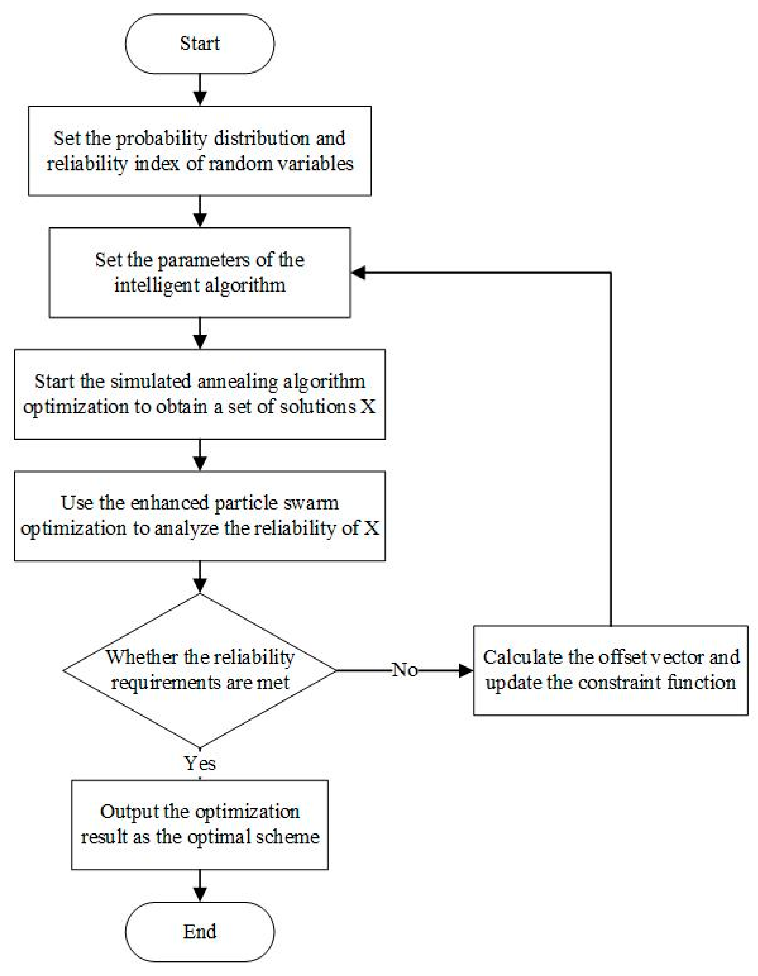
3.4. The Proposed RBDO Method Based on the PSO and SA Algorithm
- Step 1: Set the probability distribution of random variables and the reliability index of the target ;
- Step 2: Set parameters of the PSO algorithm and SA algorithm;
- Step 3: Enter the optimization cycle of the SA algorithm. Select the design variable set in step (1) as the initial point to calculate the value of the objective function;
- Step 4: Reliability analysis is carried out on the results obtained in step (3). The improved PSO algorithm is used to solve the MPP points, calculate the reliability index, and judge its reliability. If the reliability requirements are met, this solution is output as the optimal solution. Otherwise, calculate the offset vector, update the probability constraint function, and return to step (3) for a new round of reliability optimization.
| Set initial variables |
| While1 Reliability index not met %%Obtain the optimal solution space through annealing method Using simulated annealing method to generate initial solution space Random number generator initialization While2 Does not meet Metropolis criterion Equation (7) For From 1 to the set number of annealing times Generate random perturbations to obtain new solutions Check whether the Metropolis criterion Equation (7) is met, if so, exit the current annealing Perform annealing and save the optimal solution during the annealing process. End for loop Update random number generator End the while2 loop and obtain the optimal design variable solution space %%Using PSO algorithm to find MPP points %%Perform the following operations for each limit state function Initialize the population position and velocity according to the optimal solution space obtained by the annealing algorithm While3 The current iteration is less than the maximum number of iterations Update the population position and velocity according to the objective function value of each population particle Dealing with boundary issues End the current while3 loop Translational failure boundary Solve to obtain the optimal MPP point Use this point as the initial solution space for the next cycle. End the while1 loop |
4. Experimental Results and Discussion
4.1. Example Verification
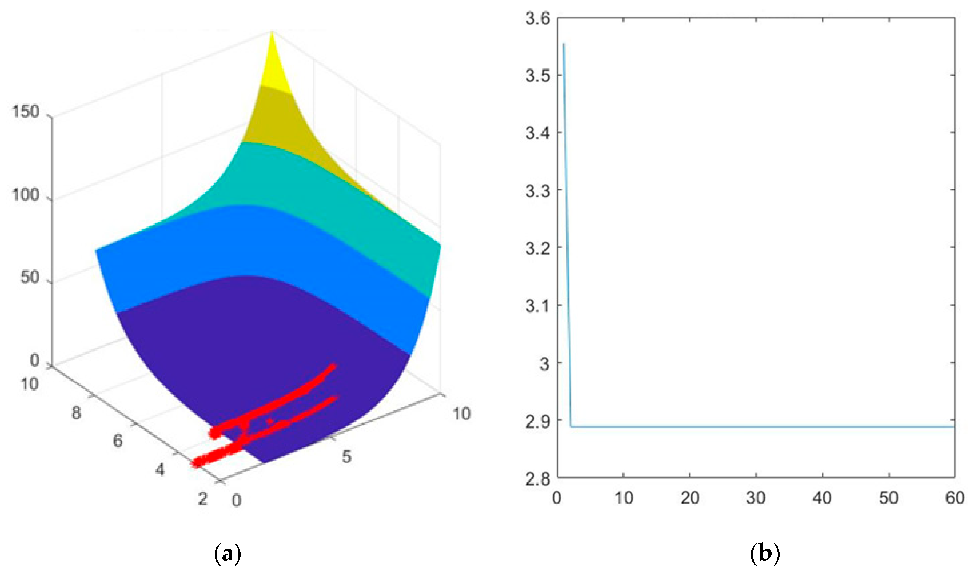
4.1.1. Convex Limit State Function
4.1.2. Concave Limit State Function
4.2. Mathematical Example
4.3. Volume Optimization of Gear Reducer
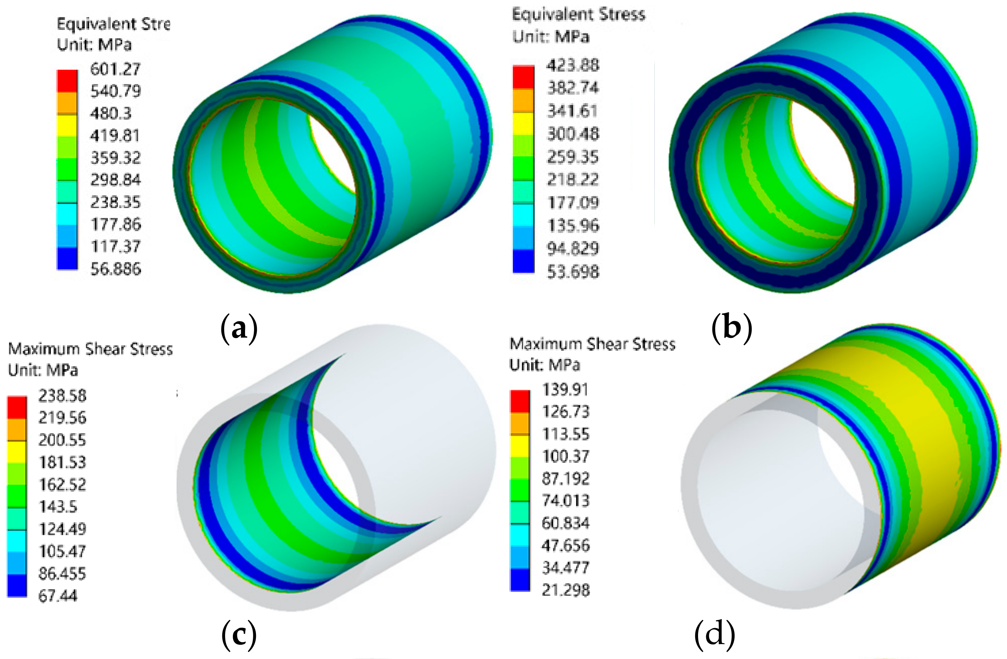
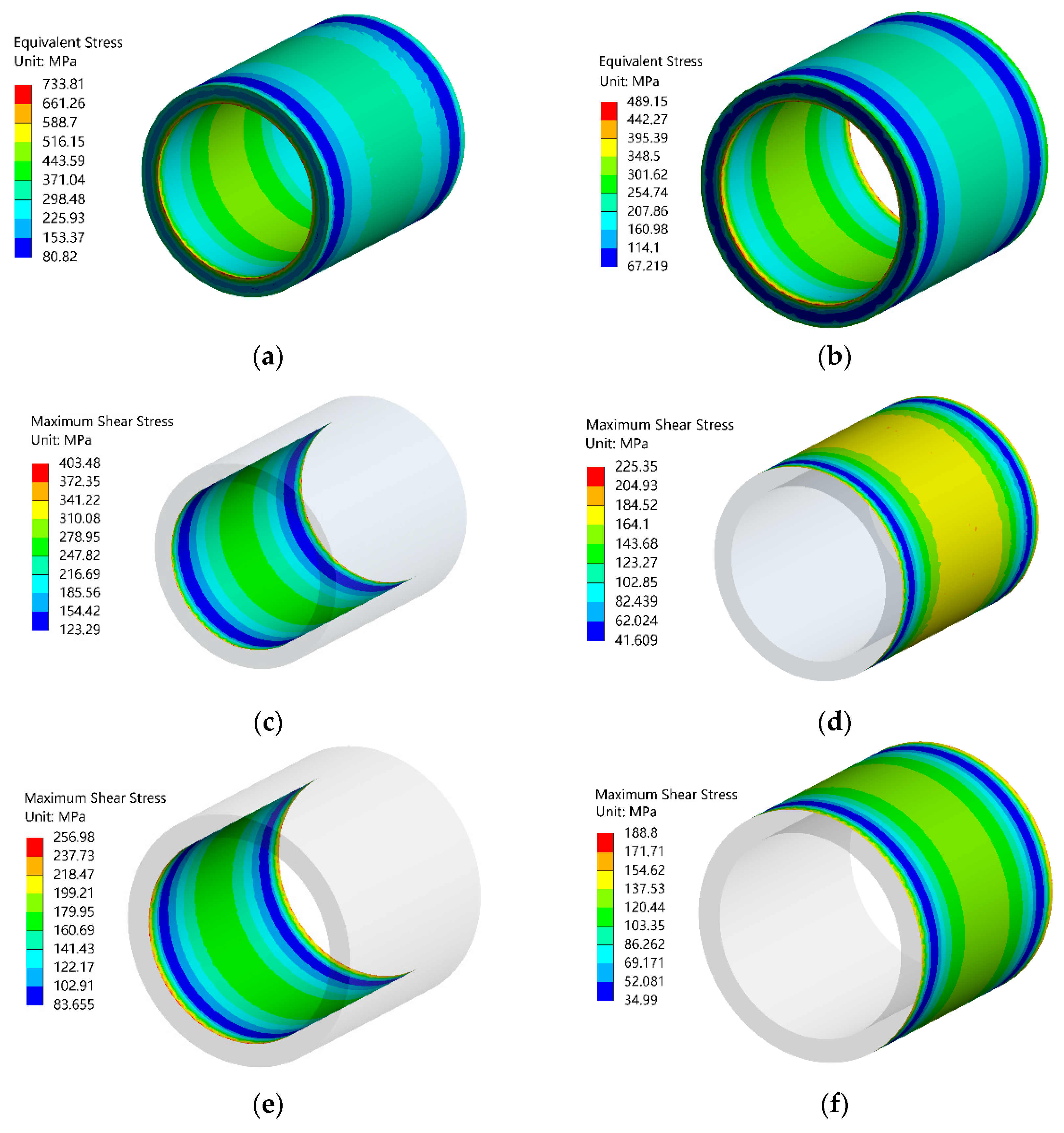
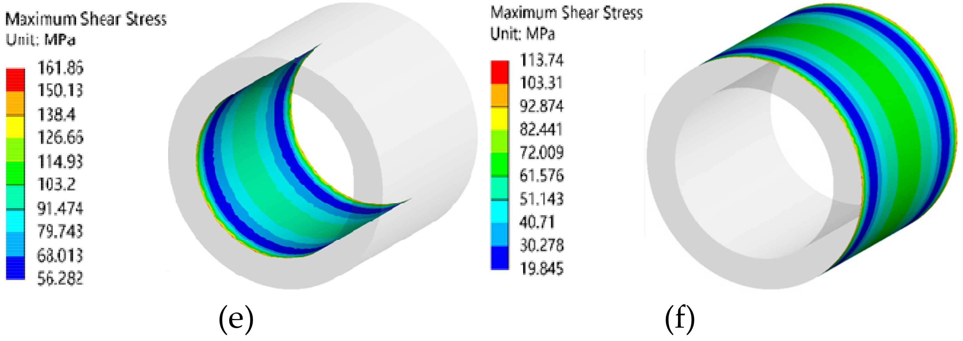
4.4. Composite Cylinder Size Optimization
5. Conclusions
Author Contributions
Funding
Data Availability Statement
Conflicts of Interest
References
- Zhong, Y.; Chen, Z.; Zhou, Z.; Hu, H. Uncertainty analysis and resource allocation in construction project management. Eng. Manag. J. 2018, 30, 293–305. [Google Scholar] [CrossRef]
- Zhu, Q. Nonlinear Systems: Dynamics, Control, Optimization and Applications to the Science and Engineering. Mathematics 2022, 10, 4837. [Google Scholar] [CrossRef]
- Meng, D.; Yang, S.; He, C.; Wang, H.; Lv, Z.; Guo, Y.; Nie, P. Multidisciplinary design optimization of engineering systems under uncertainty: A review. Int. J. Struct. Integr. 2022, 13, 565–593. [Google Scholar] [CrossRef]
- Tan, Y.; Zhan, C.; Pi, Y.; Zhang, C.; Song, J.; Chen, Y.; Golmohammadi, A.M. A Hybrid Algorithm Based on Social Engineering and Artificial Neural Network for Fault Warning Detection in Hydraulic Turbines. Mathematics 2023, 11, 2274. [Google Scholar] [CrossRef]
- Xue, Y.; Deng, Y. Extending set measures to orthopair fuzzy sets. Int. J. Uncertain. Fuzziness Knowl.-Based Syst. 2022, 30, 63–91. [Google Scholar] [CrossRef]
- Zhu, S.P.; Keshtegar, B.; Bagheri, M.; Hao, P.; Trung, N.T. Novel hybrid robust method for uncertain reliability analysis using finite conjugate map. Comput. Methods Appl. Mech. Eng. 2020, 371, 113309. [Google Scholar] [CrossRef]
- Bagheri, M.; Zhu, S.P.; Ben Seghier, M.E.A.; Keshtegar, B.; Trung, N.T. Hybrid intelligent method for fuzzy reliability analysis of corroded X100 steel pipelines. Eng. Comput. 2021, 37, 2559–2573. [Google Scholar] [CrossRef]
- Plotnikov, L. Preparation and Analysis of Experimental Findings on the Thermal and Mechanical Characteristics of Pulsating Gas Flows in the Intake System of a Piston Engine for Modelling and Machine Learning. Mathematics 2023, 11, 1967. [Google Scholar] [CrossRef]
- Zhang, D.; Zhang, J.; Yang, M.; Wang, R.; Wu, Z. An enhanced finite step length method for structural reliability analysis and reliability-based design optimization. Struct. Multidiscip. Optim. 2022, 65, 231. [Google Scholar] [CrossRef]
- Meng, D.; Yang, S.; De Jesus, A.M.; Fazeres-Ferradosa, T.; Zhu, S.P. A novel hybrid adaptive Kriging and water cycle algorithm for reliability-based design and optimization strategy: Application in offshore wind turbine monopile. Comput. Methods Appl. Mech. Eng. 2023, 412, 116083. [Google Scholar] [CrossRef]
- Yang, I.T.; Hsieh, Y.H. Reliability-based design optimization with discrete design variables and non-smooth performance functions: AB-PSO algorithm. Autom. Constr. 2011, 20, 610–619. [Google Scholar] [CrossRef]
- Yang, M.; Zhang, D.; Wang, F.; Han, X. Efficient local adaptive Kriging approximation method with single-loop strategy for reliability-based design optimization. Comput. Methods Appl. Mech. Eng. 2022, 390, 114462. [Google Scholar] [CrossRef]
- Meng, Z.; Li, G.; Wang, B.P.; Hao, P. A hybrid chaos control approach of the performance measure functions for reliability-based design optimization. Comput. Struct. 2015, 146, 32–43. [Google Scholar] [CrossRef]
- Wang, Z.; Zhao, D.; Guan, Y. Flexible-constrained time-variant hybrid reliability-based design optimization. Struct. Multidiscip. Optim. 2023, 66, 89. [Google Scholar] [CrossRef]
- Dui, H.; Song, J.; Zhang, Y.A. Reliability and Service Life Analysis of Airbag Systems. Mathematics 2023, 11, 434. [Google Scholar] [CrossRef]
- Zhang, D.; Shen, S.; Jiang, C.; Han, X.; Li, Q. An advanced mixed-degree cubature formula for reliability analysis. Comput. Methods Appl. Mech. Eng. 2022, 400, 115521. [Google Scholar] [CrossRef]
- Meng, Z.; Li, H.; Zeng, R.; Mirjalili, S.; Yıldız, A.R. An efficient two-stage water cycle algorithm for complex reliability-based design optimization problems. Neural Comput. Appl. 2022, 34, 20993–21013. [Google Scholar] [CrossRef]
- Liao, K.W.; Lu, B.C.; Yu, S.P. A Concurrent Approach for a Reliability-Based Optimization Design Problem. J. Adv. Mech. Des. Syst. Manuf. 2012, 6, 1015–1030. [Google Scholar] [CrossRef]
- Wang, Z.; Zhang, Y.; Song, Y. A modified conjugate gradient approach for reliability-based design optimization. IEEE Access 2020, 8, 16742–16749. [Google Scholar] [CrossRef]
- Safaeian Hamzehkolaei, N.; Miri, M.; Rashki, M. An enhanced simulation-based design method coupled with meta-heuristic search algorithm for accurate reliability-based design optimization. Eng. Comput. 2016, 32, 477–495. [Google Scholar] [CrossRef]
- Zhong, C.; Wang, M.; Dang, C.; Ke, W.; Guo, S. First-order reliability method based on Harris Hawks Optimization for high-dimensional reliability analysis. Struct. Multidiscip. Optim. 2020, 62, 1951–1968. [Google Scholar] [CrossRef]
- Jafari-Asl, J.; Seghier, M.E.A.B.; Ohadi, S.; Correia, J.; Barroso, J. Reliability analysis based improved directional simulation using Harris Hawks optimization algorithm for engineering systems. Eng. Fail. Anal. 2022, 135, 106148. [Google Scholar] [CrossRef]
- Du, X.P.; Sudjianto, A.; Huang, B.Q. Reliability-based design with the mixture of random and interval variables. J. Mech. Des. 2005, 127, 1068–1076. [Google Scholar] [CrossRef]
- Zhang, H.; Wang, H.; Wang, Y.; Hong, D. Incremental shifting vector and mixed uncertainty analysis method for reliability-based design optimization. Struct. Multidiscip. Optim. 2019, 59, 2093–2109. [Google Scholar] [CrossRef]
- Wang, L.; Ma, Y.; Yang, Y.; Wang, X. Structural design optimization based on hybrid time-variant reliability measure under non-probabilistic convex uncertainties. Appl. Math. Model. 2019, 69, 330–354. [Google Scholar] [CrossRef]
- Van Huynh, T.; Tangaramvong, S.; Do, B.; Gao, W.; Limkatanyu, S. Sequential most probable point update combining Gaussian process and comprehensive learning PSO for structural reliability-based design optimization. Reliab. Eng. Syst. Saf. 2023, 235, 109164. [Google Scholar] [CrossRef]
- Keshtegar, B.; Chakraborty, S. A hybrid self-adaptive conjugate first order reliability method for robust structural reliability analysis. Appl. Math. Model. 2018, 53, 319–332. [Google Scholar] [CrossRef]
- Bartoccini, U.; Carpi, A.; Poggioni, V.; Santucci, V. Memes evolution in a memetic variant of particle swarm optimization. Mathematics 2019, 7, 423. [Google Scholar] [CrossRef]
- Li, J.; Chen, J. Solving time-variant reliability-based design optimization by PSO-t-IRS: A methodology incorporating a particle swarm optimization algorithm and an enhanced instantaneous response surface. Reliab. Eng. Syst. Saf. 2019, 191, 106580. [Google Scholar] [CrossRef]
- Zhang, Y.; Liu, X.; Li, C. Determining the reasonable state of cable-stayed bridges with twin towers based on multi-objective swarm optimization algorithm. J. Chang. Univ. Sci. Technol. (Nat. Sci.) 2019, 16, 22–27. [Google Scholar]
- Zhu, S.P.; Keshtegar, B.; Seghier, M.E.A.B.; Zio, E.; Taylan, O. Hybrid and enhanced PSO: Novel first order reliability method-based hybrid intelligent approaches. Comput. Methods Appl. Mech. Eng. 2022, 393, 114730. [Google Scholar] [CrossRef]
- Yu, S.; Wang, Z. A general decoupling approach for time-and space-variant system reliability-based design optimization. Comput. Methods Appl. Mech. Eng. 2019, 357, 112608. [Google Scholar] [CrossRef]
- Wang, C.; Matthies, H.G. A comparative study of two interval-random models for hybrid uncertainty propagation analysis. Mech. Syst. Signal Process. 2020, 136, 106531. [Google Scholar] [CrossRef]
- Chopard, B.; Tomassini, M.; Chopard, B.; Tomassini, M. Simulated annealing. In An Introduction to Metaheuristics for Optimization; Springer: Berlin/Heidelberg, Germany, 2018; pp. 59–79. [Google Scholar]
- Alnowibet, K.A.; Mahdi, S.; El-Alem, M.; Abdelawwad, M.; Mohamed, A.W. Guided hybrid modified simulated annealing algorithm for solving constrained global optimization problems. Mathematics 2022, 10, 1312. [Google Scholar] [CrossRef]
- Liu, X.; Liu, X.; Zhou, Z.; Hu, L. An efficient multi-objective optimization method based on the adaptive approximation model of the radial basis function. Struct. Multidiscip. Optim. 2021, 63, 1385–1403. [Google Scholar] [CrossRef]
- Delahaye, D.; Chaimatanan, S.; Mongeau, M. Simulated annealing: From basics to applications. In Handbook of Metaheuristics; Springer: Berlin/Heidelberg, Germany, 2019; pp. 1–35. [Google Scholar]
- Franzin, A.; Stützle, T. Revisiting simulated annealing: A component-based analysis. Comput. Oper. Res. 2019, 104, 191–206. [Google Scholar] [CrossRef]
- Liu, X.; Gong, M.; Zhou, Z.; Xie, J.; Wu, W. An improved first order approximate reliability analysis method for uncertain structures based on evidence theory. Mech. Based Des. Struct. Mach. 2023, 51, 4137–4154. [Google Scholar] [CrossRef]
- Wang, Q.; Huang, Z.; Dong, J. Reliability-based design optimization for vehicle body crashworthiness based on copula functions. Eng. Optim. 2020, 52, 1362–1381. [Google Scholar] [CrossRef]
- Ai, Q.; Yuan, Y.; Jiang, X.; Wang, H.; Han, C.; Huang, X.; Wang, K. Pathological diagnosis of the seepage of a mountain tunnel. Tunn. Undergr. Space Technol. 2022, 128, 104657. [Google Scholar] [CrossRef]
- Li, W.; Li, C.; Gao, L.; Xiao, M. Risk-based design optimization under hybrid uncertainties. Eng. Comput. 2020, 38, 2037–2049. [Google Scholar] [CrossRef]
- Liu, X.; Li, T.; Zhou, Z.; Hu, L. An efficient multi-objective reliability-based design optimization method for structure based on probability and interval hybrid model. Comput. Methods Appl. Mech. Eng. 2022, 392, 114682. [Google Scholar] [CrossRef]
- Luo, C.; Keshtegar, B.; Zhu, S.P.; Taylan, O.; Niu, X.P. Hybrid enhanced Monte Carlo simulation coupled with advanced machine learning approach for accurate and efficient structural reliability analysis. Comput. Methods Appl. Mech. Eng. 2022, 388, 114218. [Google Scholar] [CrossRef]
- Liu, X.; Lai, H.; Wang, X.; Song, X.; Liu, K.; Wu, S.; Li, Q.; Wang, F.; Zhou, Z. Aerospace Structural Reliability Analysis Method Based on Regular Vine Copula Model with the Asymmetric Tail Correlation. Aerosp. Sci. Technol. 2023, 142, 108670. [Google Scholar] [CrossRef]
- Thakkar, A.; Lohiya, R. A survey on intrusion detection system: Feature selection, model, performance measures, application perspective, challenges, and future research directions. Artif. Intell. Rev. 2022, 55, 453–563. [Google Scholar] [CrossRef]
- Wang, Y.H.; Zhang, C.; Su, Y.Q.; Shang, L.Y.; Zhang, T. Structure optimization of the frame based on response surface method. Int. J. Struct. Integr. 2019, 11, 411–425. [Google Scholar] [CrossRef]
- Yang, S.; Meng, D.; Wang, H.; Chen, Z.; Xu, B. A comparative study for adaptive surrogate-model-based reliability evaluation method of automobile components. Int. J. Struct. Integr. 2023, 14, 498–519. [Google Scholar] [CrossRef]
- Meng, D.; Yang, S.; de Jesus, A.M.; Zhu, S.P. A novel Kriging-model-assisted reliability-based multidisciplinary design optimization strategy and its application in the offshore wind turbine tower. Renew. Energy 2023, 203, 407–420. [Google Scholar] [CrossRef]
- Chen, J.; Zhang, X.; Jing, Z. A cooperative PSO-DP approach for the maintenance planning and RBDO of deteriorating structures. Struct. Multidiscip. Optim. 2018, 58, 95–113. [Google Scholar] [CrossRef]
- Lai, X.; Huang, J.; Zhang, Y.; Wang, C.; Zhang, X. A general methodology for reliability-based robust design optimization of computation-intensive engineering problems. J. Comput. Des. Eng. 2022, 9, 2151–2169. [Google Scholar] [CrossRef]
- Qiang, C.; Deng, Y. A new correlation coefficient of mass function in evidence theory and its application in fault diagnosis. Appl. Intell. 2022, 52, 7832–7842. [Google Scholar] [CrossRef]
- Ai, Q.; Yuan, Y.; Shen, S.L.; Wang, H.; Huang, X. Investigation on inspection scheduling for the maintenance of tunnel with different degradation modes. Tunn. Undergr. Space Technol. 2020, 106, 103589. [Google Scholar] [CrossRef]
- Gao, J.W.; Dai, X.; Zhu, S.P.; Zhao, J.W.; Correia, J.A.; Wang, Q. Failure causes and hardening techniques of railway axles—A review from the perspective of structural integrity. Eng. Fail. Anal. 2022, 141, 106656. [Google Scholar] [CrossRef]
- Yang, S.; Meng, D.; Wang, H.; Yang, C. A novel learning function for adaptive surrogate-model-based reliability evaluation. Philos. Trans. R. Soc. A 2023, 382, 20220395. [Google Scholar] [CrossRef] [PubMed]
- Xiong, L.; Su, X.; Qian, H. Conflicting evidence combination from the perspective of networks. Inf. Sci. 2021, 580, 408–418. [Google Scholar] [CrossRef]
- Yu, S.; Li, Y. Active learning kriging model with adaptive uniform design for time-dependent reliability analysis. IEEE Access 2021, 9, 91625–91634. [Google Scholar] [CrossRef]
- Gao, X.; Su, X.; Qian, H.; Pan, X. Dependence assessment in human reliability analysis under uncertain and dynamic situations. Nucl. Eng. Technol. 2022, 54, 948–958. [Google Scholar] [CrossRef]
- Meng, Z.; Keshtegar, B. Adaptive conjugate single-loop method for efficient reliability-based design and topology optimization. Comput. Methods Appl. Mech. Eng. 2019, 344, 95–119. [Google Scholar] [CrossRef]
- Li, W.; Xiao, M.; Garg, A.; Gao, L. A New Approach to Solve Uncertain Multidisciplinary Design Optimization based on Conditional Value at Risk. IEEE Trans. Autom. Sci. Eng. 2021, 18, 356–368. [Google Scholar] [CrossRef]
- Meng, D.; Yang, S.; Lin, T.; Wang, J.; Yang, H.; Lv, Z. RBMDO using gaussian mixture model-based second-order mean-value saddlepoint approximation. Comput. Model. Eng. Sci. 2022, 132, 553–568. [Google Scholar] [CrossRef]
- Li, X.Q.; Song, L.K.; Bai, G.C. Recent advances in reliability analysis of aeroengine rotor system: A review. Int. J. Struct. Integr. 2021, 13, 1–29. [Google Scholar] [CrossRef]
- Yang, S.; Meng, D.; Guo, Y.; Nie, P.; Jesus, A.M.D. A reliability-based design and optimization strategy using a novel MPP searching method for maritime engineering structures. Int. J. Struct. Integr. 2023, 14, 809–826. [Google Scholar] [CrossRef]
- Lu, L.; Wu, Y.; Zhang, Q.; Qiao, P. A Transformation-Based Improved Kriging Method for the Black Box Problem in Reliability-Based Design Optimization. Mathematics 2023, 11, 218. [Google Scholar] [CrossRef]
- Song, L.K.; Bai, G.C.; Li, X.Q.; Wen, J. A unified fatigue reliability-based design optimization framework for aircraft turbine disk. Int. J. Fatigue 2021, 152, 106422. [Google Scholar] [CrossRef]
- Song, X.; Xiao, F. Combining time-series evidence: A complex network model based on a visibility graph and belief entropy. Appl. Intell. 2022, 52, 10706–10715. [Google Scholar] [CrossRef]
- Song, K.; Zhang, Y.; Zhuang, X.; Yu, X.; Song, B. Reliability-based design optimization using adaptive surrogate model and importance sampling-based modified SORA method. Eng. Comput. 2021, 37, 1295–1314. [Google Scholar] [CrossRef]
- Wang, Z.; Xiao, F.; Cao, Z. Uncertainty measurements for Pythagorean fuzzy set and their applications in multiple-criteria decision making. Soft Comput. 2022, 26, 9937–9952. [Google Scholar] [CrossRef]
- Dunn, W.L.; Shultis, J.K. Exploring Monte Carlo Methods, 3rd ed.; Elsevier: Burlington, MA, USA, 2012; pp. 154–196. [Google Scholar]
- Liang, J.; Mourelatos, Z.P.; Tu, J. A single-Loop method for reliability-based design optimization. Proc. ASME Des. Eng. Tech. Conf. 2004, 1, 419–430. [Google Scholar]
- Azarm, S.; Li, W.C. Multi-level design optimization using global monotonicity analysis. J. Mech. Transm. Autom. Des. 1989, 111, 259–263. [Google Scholar] [CrossRef]
- Gunawan, S.; Azarm, S.; Wu, J.; Boyars, A. Quality-assisted multi-objective multidisciplinary genetic algorithms. Aiaa J. 2003, 41, 1752–1762. [Google Scholar] [CrossRef]


| The PSO Algorithm | |
|---|---|
| Step 1 | Firstly, PSO is used to generate a set of initial solutions; |
| Step 2 | For each particle, the value of its objective function is calculated and the current optimal solution is recorded; |
| Step 3 | Calculate the speed of each particle, according to the speed of updating the positions of the particles in the solution space; |
| Step 4 | Using the Metropolis criterion to decide whether to accept the new position; |
| Step 5 | The particles are updated in a certain order to make the local optimal particle position move to the global optimal, which improves the global search performance of the algorithm |
| Step 6 | Repeat Steps 2 through 5 until the termination condition is reached |
| Method | Reliability Index | Error | Solution Time (Milliseconds) |
|---|---|---|---|
| MCS | 2.8445 | −− | 1,948,731.39 |
| SQP | 2.8782 | 1.2% | 988.71 |
| Improved PSO | 2.8865 | 1.5% | 47.67 |
| Method | Reliability Index | Error | Solution Time (Milliseconds) |
|---|---|---|---|
| MCS | 2.9906 | −− | 1,851,997.89 |
| SQP | 2.1681 | 27.5% | 80.32 |
| Improved PSO | 2.8891 | 3.4% | 228.12 |
| Method | Optimal Solution | Error | Solution Time (Milliseconds) |
|---|---|---|---|
| Theoretical method | 6.7318 | −− | −− |
| SQP | 7.4195 | 10.2% | 320.5 |
| GA | 6.9754 | 3.6% | 6975.4 |
| The proposed method | 7.0988 | 5.5% | 211.9 |
| Design Variable | Mean Value | Standard Deviation | Distribution Type | Lower Bound of Mean | Upper Bound of Mean |
|---|---|---|---|---|---|
| Tooth width factor | Orthographic distribution | 2.63 | 3.57 | ||
| Module of gear teeth | Orthographic distribution | 0.71 | 0.81 | ||
| Number of teeth of gear 1 | Orthographic distribution | 17 | 23 | ||
| Length of shaft 1 | Orthographic distribution | 7.31 | 8.29 | ||
| Length of shaft 2 | Orthographic distribution | 7.31 | 8.29 | ||
| Shaft 1 diameter | Orthographic distribution | 2.93 | 3.87 | ||
| Shaft 2 diameter | Orthographic distribution | 5.03 | 5.47 |
| Design Variable | Upper Bound of Interval | Lower Bound of Interval |
|---|---|---|
| Shaft 1 diameter | 2.93 | 3.87 |
| Shaft 1 diameter | 5.03 | 5.47 |
| Uncertainty Description | Optimal Solution | Error |
|---|---|---|
| Comparison method(MCS) | 2753.8 | |
| SQP | 2851.2653 | 3.54% |
| GA | 2891.1236 | 4.99% |
| The proposed method 1 | 2773.0126 | 0.69% |
| The proposed method 2 | 2814.9546 | 2.22% |
| Name | Symbol | Value |
|---|---|---|
| Modulus of elasticity/GPa | 210 | |
| Poisson’s ratio | 0.3 | |
| Internal pressure/MPa | 139.7 | |
| Allowable stress/MPa | 607.7 | |
| Allowable shear stress/MPa | 244.5 |
| a | b | c | |||||||
|---|---|---|---|---|---|---|---|---|---|
| 1 | 38.5 | 39.9 | 49.7 | 889.90 | 997.82 | 483.00 | 400.66 | 526.84 | 346.94 |
| 2 | 39.2 | 49.6 | 53.1 | 1069.30 | 518.25 | 578.87 | 273.39 | 273.69 | 180.97 |
| 3 | 33.0 | 49.5 | 55.5 | 589.82 | 252.57 | 324.35 | 130.22 | 133.18 | 89.94 |
| 4 | 39.3 | 43.8 | 58.0 | 792.55 | 528.81 | 441.83 | 281.42 | 279.47 | 186.87 |
| 5 | 37.1 | 47.6 | 50.4 | 751.12 | 438.64 | 414.24 | 234.62 | 230.51 | 177.81 |
| 6 | 32.8 | 39.7 | 52.7 | 605.15 | 391.49 | 337.28 | 195.88 | 207.00 | 135.23 |
| 7 | 34.2 | 43.1 | 52.3 | 811.37 | 436.74 | 442.53 | 218.96 | 231.57 | 170.05 |
| 8 | 36.4 | 49.0 | 56.8 | 881.32 | 430.42 | 483.57 | 201.98 | 226.71 | 155.63 |
| 9 | 39.7 | 47.5 | 49.7 | 1256.80 | 565.43 | 675.41 | 353.23 | 308.07 | 260.49 |
| 10 | 39.7 | 49.5 | 55.1 | 990.28 | 564.01 | 536.79 | 274.83 | 297.29 | 199.18 |
| 1,306,319 | 41,973.2 | 685,669.2 | 116,143.7 | 34,266.6 | −23,063.3 | |
| −34,404 | −644.3 | −18,032.3 | −2974.9 | −663.4 | 748.8 | |
| −28,761.7 | −1219.7 | −15,093.5 | −2522.8 | −894.6 | 502.7 | |
| −24,292.4 | −753.5 | −12,764.2 | −2184.7 | −628.1 | 367.9 | |
| −5 | −1.7 | −3 | 0.8 | −0.7 | 0.6 | |
| −10.9 | 0.5 | −5.5 | −1.1 | 0.01 | −1.7 | |
| −9.4 | −3.1 | −4.7 | −0.4 | −1.5 | 0.3 | |
| 761.1 | 18.5 | 399.3 | 65.2 | 16.7 | −14 | |
| 645.8 | 18.3 | 339 | 55.2 | 15.2 | −14.6 | |
| 550.9 | 23.7 | 288.7 | 48.9 | 17.5 | −6.8 | |
| −14.1 | −0.4 | −7.4 | −1.2 | −0.3 | 0.3 |
| Variable | ||||
|---|---|---|---|---|
| GA | 37.65 | 38.10 | 59.58 | 55,662.18 |
| SQP | 38.47 | 38.10 | 59.26 | 57,190.73 |
| Result | 37.40 | 45.72 | 60.96 | 54,929.13 |
Disclaimer/Publisher’s Note: The statements, opinions and data contained in all publications are solely those of the individual author(s) and contributor(s) and not of MDPI and/or the editor(s). MDPI and/or the editor(s) disclaim responsibility for any injury to people or property resulting from any ideas, methods, instructions or products referred to in the content. |
© 2023 by the authors. Licensee MDPI, Basel, Switzerland. This article is an open access article distributed under the terms and conditions of the Creative Commons Attribution (CC BY) license (https://creativecommons.org/licenses/by/4.0/).
Share and Cite
Yang, S.; Wang, H.; Xu, Y.; Guo, Y.; Pan, L.; Zhang, J.; Guo, X.; Meng, D.; Wang, J. A Coupled Simulated Annealing and Particle Swarm Optimization Reliability-Based Design Optimization Strategy under Hybrid Uncertainties. Mathematics 2023, 11, 4790. https://doi.org/10.3390/math11234790
Yang S, Wang H, Xu Y, Guo Y, Pan L, Zhang J, Guo X, Meng D, Wang J. A Coupled Simulated Annealing and Particle Swarm Optimization Reliability-Based Design Optimization Strategy under Hybrid Uncertainties. Mathematics. 2023; 11(23):4790. https://doi.org/10.3390/math11234790
Chicago/Turabian StyleYang, Shiyuan, Hongtao Wang, Yihe Xu, Yongqiang Guo, Lidong Pan, Jiaming Zhang, Xinkai Guo, Debiao Meng, and Jiapeng Wang. 2023. "A Coupled Simulated Annealing and Particle Swarm Optimization Reliability-Based Design Optimization Strategy under Hybrid Uncertainties" Mathematics 11, no. 23: 4790. https://doi.org/10.3390/math11234790
APA StyleYang, S., Wang, H., Xu, Y., Guo, Y., Pan, L., Zhang, J., Guo, X., Meng, D., & Wang, J. (2023). A Coupled Simulated Annealing and Particle Swarm Optimization Reliability-Based Design Optimization Strategy under Hybrid Uncertainties. Mathematics, 11(23), 4790. https://doi.org/10.3390/math11234790