1. Introduction and Motivations
Since a few centuries ago, many distinct definitions of fractional operators have been introduced [
1]. Following the initial Riemann–Liouville definition in 1645 [
2,
3], several other definitions appeared. To mention a few different definitions, we have: Weyl [
4], Caputo [
5], Caputo–Fabrizio [
6], Canavati [
7], Riesz [
8], Hilfer [
9], Erdélyi–Kober [
10], Jumarie [
11], Atangana–Baleanu [
12], Davidson–Essex [
13], Yang [
14], Miller—Ross [
15], Marchaud [
16], Hadamard [
17], Osler [
18], Cossar [
19], Sonin—Letnikov [
1], Coimbra [
20], Katugampola [
21], Hilfer–Katugampola [
22], and Grünwald–Letnikov [
23]. The number of distinct fractional operators is becoming so large that the need to classify them on subsets has been studied [
24].
Integer operators acting on a function are local operators (the value can be computed using only knowledge of the values of in an arbitrarily small neighborhood around x), while fractional operators are typically introduced as non-local operators (the value provided depends on the domain definition or on the definition of an initial point). The fractional operators so-far introduced are derived as the extension of some specific mathematical definition with the hope that it is supposed valid also for fractional operators of any order. For example, the definition of the Riemann–Liouville fractional operators comes from the Cauchy formula for repeated integration, while the definition of the Grünwald–Letnikov comes from the limit of finite differences. Unfortunately, the existing fractional operators also depend on the selection of an initial point, and this generates continuity issues at that point. How can this loss of continuity be justified?
Calculus is mainly based on the concepts of two operators: the derivative and its inverse, the anti-derivative. Based on the anti-derivative, definite, indefinite integrals can be derived. The integer operators have a clear and known geometrical meaning. By contrast, the geometrical meaning of all fractional operators so-far introduced is still questionable. To give some examples, ref. [
25] has provided the geometrical interpretation using a new specific definition of fractional derivatives; ref. [
26] has shown that for the Riemann–Liouville derivatives, a connection with infinite jet bundles, the interpretation given by [
27] is restricted to polynomial functions only; meanwhile the interpretation for [
28] is based on the four concepts of fractal geometry, linear filters, construction of a Cantor set, and physical realization of fractional operators.
The proliferation of fractional operator definitions has generated confusion, ambiguity, and uncertainty among users, with consequent delayed research and disinterest in the subject. The main reason is: the user should know which one suits the problem he wants to solve. An answer to this question requires knowing all existing formulations, their ranges of definition, and their assumptions. What if the user’s domain of application does not match with any of the fractional operators’ existing domains? Or what if the problem under analysis does not suggest the selection of an initial point, which is often required by the various formulations? In addition, to implement the existing fractional operators, the computation of complicated integrals and/or infinite series, such as the Mittag–Leffler function [
29,
30], is needed. Closed-form expressions of fractional operators do exist but just for a very small subset of basic functions and for some specific formulations only [
31].
However, despite these difficulties, the number of applications of fractional calculus is slowly increasing and is touching many science and engineering problems [
32]. On the other hand, no specific reason exists to support that the equations governing physical problems must involve integer operators only. This article is based on the fundamental constraint of any fractional operator: it must provide the expression given by the integer operator when the fractional operator variable becomes an integer. Therefore, due to the flourishing of applications involving fractional operators, this article aims to provide an approximate, flexible, and easy mathematical tool that can be used for any function with no mathematical and/or computational issues for users. This is done by facing the problem of fractional operators from an interpolation point of view. Specifically, the interpolation tool used is the one provided by the Theory of Functional Connections (TFC) [
33,
34,
35,
36].
Using TFC, the set of constraints defined by integer derivatives and/or integrals are (1) analytically satisfied and (2) all possible functions interpolating the constraints can be obtained. This implies that the proposed method can be used to simulate all possible fractional operators. Specifically, these approximations are obtained using the flexibility of orthogonal polynomials and the power of least-squares. However, different minimization techniques and different ways to expand the free function by, for instance, using neural networks [
37,
38], can also be successfully used. Basically, the purpose of this article is to provide a simple and practical approach for anyone interested in exploring the infinite possibilities offered by morphing integer operators between consecutive values: that is, by the infinite continuous transitions between the well-known integer operators—transitions that are explored using a tool, the TFC [
33,
34,
35,
36], able to provide
all of these infinite transitions.
To summarize: the main contribution of this article consists of providing a functional interpolation tool (TFC) to derive all possible continuous variations between continuous integer derivatives and/or integrals. This includes the continuous variations provided by the existing fractional operators. Using the same mathematical tool, this article provides all continuous functions fitting discrete series and all continuous surfaces fitting series of functions.
1.1. Notations
In this article, indicates a generic fractional derivative (if ) or antiderivative (if ) applied to the function . The approximated function obtained by TFC is indicated by the surface where the additional variable () retains the meaning of the fractional operator variable. This means that , , is the anti-derivative of , and is the indefinite integral of with the initial point a.
Function identifies a surface constrained by the boundary conditions , where , indicating the integer derivatives and/or anti-derivatives in the range of interest. Note that additional boundary conditions can be easily added to the problem under analysis. For example, for trigonometric functions, the integer derivative periodicity is described by the relative constraint , where . One can even propose extending this periodicity to , where (a false relationship for the existing fractional operators), to obtain a periodicity for any .
This proposed approach is not a new mathematical definition of fractional operators but just an interpretation of the fractional operators from the interpolation point of view. The proposed approach has the advantage of providing a continuous, simple, and practical tool to explore the infinite surfaces connecting integer operators.
The resulting surface
provided by TFC is called the
constrained expression and should actually be indicated as
because it is a functional: i.e., a function of the free function,
. By spanning all possible free functions
, this functional describes
all possible surfaces analytically satisfying the assigned boundary constraints. The resulting consequence is: in theory, any possible distinct fractional operator can be analytically replaced by a constrained expression using a specific free function. To numerically implement this proposed method, the specific free function is estimated by fitting the data provided by the fractional operator under consideration,
, by least-squares using the constrained expression. For example, the last section of this article shows the highly accurate approximation of the Mittag–Leffler function, which is extensively used to compute fractional operators [
39,
40].
In addition, this article includes the following mathematical tools:
Switching functions for integers: Since fractional operators have all constraints specified for
, a closed-form of switching functions analytically satisfying the switching function property
is developed for integers. These switching functions are computed by avoiding matrix inversion and are valid for any series of real numbers. This set of switching functions is called “Lagrangian switching functions” because their expressions coincide with the multiplicative terms of Lagrange polynomials [
41].
Continuous description of integer and function sequences: The capability of generating closed-form switching functions for integers provides us the capability to use TFC to generate all functions interpolating any numbers sequence and all surfaces interpolating any function sequence. The example of interpolating the function in the range is provided.
Finally, the accuracy of the proposed approach is validated by estimating (by least-squares) the constrained expression of the Mittag–Leffler function [
29,
30]. The reasons for this selection are (1) the boundary continuity issues affecting the existing fractional operators are in conflict with any fitting method using smooth functions, (2) the Mittag–Leffler function has no discontinuities and is a key function to compute closed-form expressions of fractional operators [
31,
42], (3) the Mittag–Leffler function has a variety of other applications [
30], and (4) because it is a complicate function to evaluate, expressed by infinite series of a
function.
1.2. Brief Background on the Theory of Functional Connections
The Theory of Functional Connections (TFC), introduced in the seminal paper [
33], performs analytical functional interpolation, which is a generalization of interpolation. The TFC derives analytical expressions with embedded constraints; these expressions describe all possible functions satisfying a set of constraints. This new mathematical framework has been extended to multivariate domains and to a wide class of constraints, including points, functions, integer and fractional derivatives/integrals, limits, components, and any linear combination of these. Applications are found in constrained optimization problems, as these functionals collapse the whole function space to just the subspace fully satisfying the constraints where the solution is located. By transforming a constrained optimization problem into an unconstrained one, the solution can be then obtained with simpler, faster, more robust, and more accurate methods. The application areas of TFC optimization include differential equations [
35,
36,
43], homotopy continuation [
44], quadratic and nonlinear programming [
45], boundary geodesic problems [
46], machine learning [
37,
38], vector spaces [
47], space object monitoring [
48], optimal control [
49,
50], and fractional operators [
51,
52,
53], just to mention the most relevant.
The univariate version of TFC can be obtained by either one of these two functionals, called ‘constrained expressions’ [
54]:
where
n is the number of constraints,
is the
free function,
is a set of
n user-defined linearly independent
support functions,
are
coefficient functionals,
are
switching functions (they are 1 when evaluated at the constraint’s coordinate they are referring to and 0 when any other constraint is satisfied), and
are
projection functionals representing the constraints written in terms of the free function. The complete explanation and the properties of the support, switching, and free functions as well as of the coefficient and projection functionals can be found in [
43,
54].
This article highlights the flexibility of these functionals not only to perform interpolation in the context of fractional operators but also to obtain continuous functions interpolating integer sequences and continuous surfaces interpolating function sequences.
3. Continuous Representations of Any Integer or Function Sequence
In mathematics and computer science, the sequence of integers and functions is an important subject. While traditional discrete integer sequences have been instrumental for solving many problems, there exists a class of challenges wherein continuous representations of them prove to be not only advantageous but often indispensable. This section shows how to derive these continuous representations by proposing a general method that enables the transitions from a discrete sequence of integers (or real or complex numbers) to a set of continuous functions and the transitions from a discrete sequence of functions to a set of continuous surfaces matching the integer and function sequences, respectively. By bridging the gap between the discrete and the continuous, a new level of flexibility in handling a wide spectrum of mathematical and computational problems can be explored.
An existing example is the function: a continuous function interpolating the sequence of factorials. Since these sequences are often infinite, a closed-form expression of an infinite set of switching functions is needed to perform functional interpolation.
3.1. Switching Functions for Sequences
Switching functions are derived by selecting
n support functions for some
n constraints. In our case, the constraints all occur when
. However, it is possible to derive the switching functions for a set of
n complex values:
. The property of the switching functions implies that the function
must be zero if
. Therefore, thanks to the fundamental theorem of algebra,
The constant
can be computed by imposing
. Therefore,
These switching functions are nothing else than the coefficient terms of Lagrange polynomials,
, interpolating the
n points,
,
The set of switching functions given by Equation (
6) satisfies the following two properties:
Proposition 1. The sum of all switching functions is 1, Proof. All are polynomials of degree ; therefore, the sum of these polynomials can be a polynomial of degree or lower but not greater. The polynomials are switching functions: therefore, for any i, we have . Therefore, the polynomial has n roots at all the and at . Therefore, the cannot be a function of . Since the polynomial has n roots, then must be satisfied for any values of . □
Proposition 2. The switching functions are linearly independent,because the Lagrange coefficients are linearly independent. In addition, it is our conjecture that the Wronskian of the switching functions matrix is 1: that is, the switching functions matrix is unimodular. It is important to outline that the generation of these Lagrange switching functions does not require any matrix inversion.
3.2. Functional Interpolation of Any Sequence of Numbers and Functions
Using Lagrange switching functions, all continuous functions interpolating any integer sequence can be obtained. For instance, the functional
interpolates the factorials. In theory, by spanning all possible expressions of the free function
,
all continuous functions interpolating factorials can be obtained. Specifically, there exists an expression of the free function that makes this functional approximate the
function. This is done in
Section 3.3 at a high accuracy level.
Similarly, the functional representing
all functions interpolating Fibonacci’s sequence is
where the Fibonacci sequence satisfies the recursive relation
. Following the same logic, this approach can be used to interpolate by continuous functions any sequence numbers [
55]: for instance, the prime numbers [
56], the Catalan numbers [
57], the Bell numbers [
58], the perfect numbers [
59], and the Abundant numbers [
60], just to mention a few. Extensive sequences can be found in the Encyclopedia of Integer Sequences [
61] and are published in the Journal of Integer Sequences [
62].
Similarly, this approach can be used to interpolate any function sequences. For instance, the functional describing
all surfaces interpolating Legendre’s orthogonal polynomials is
where
is the recursive (Bonnet’s) relation defining the sequence of Legendre’s polynomials, starting with
and
.
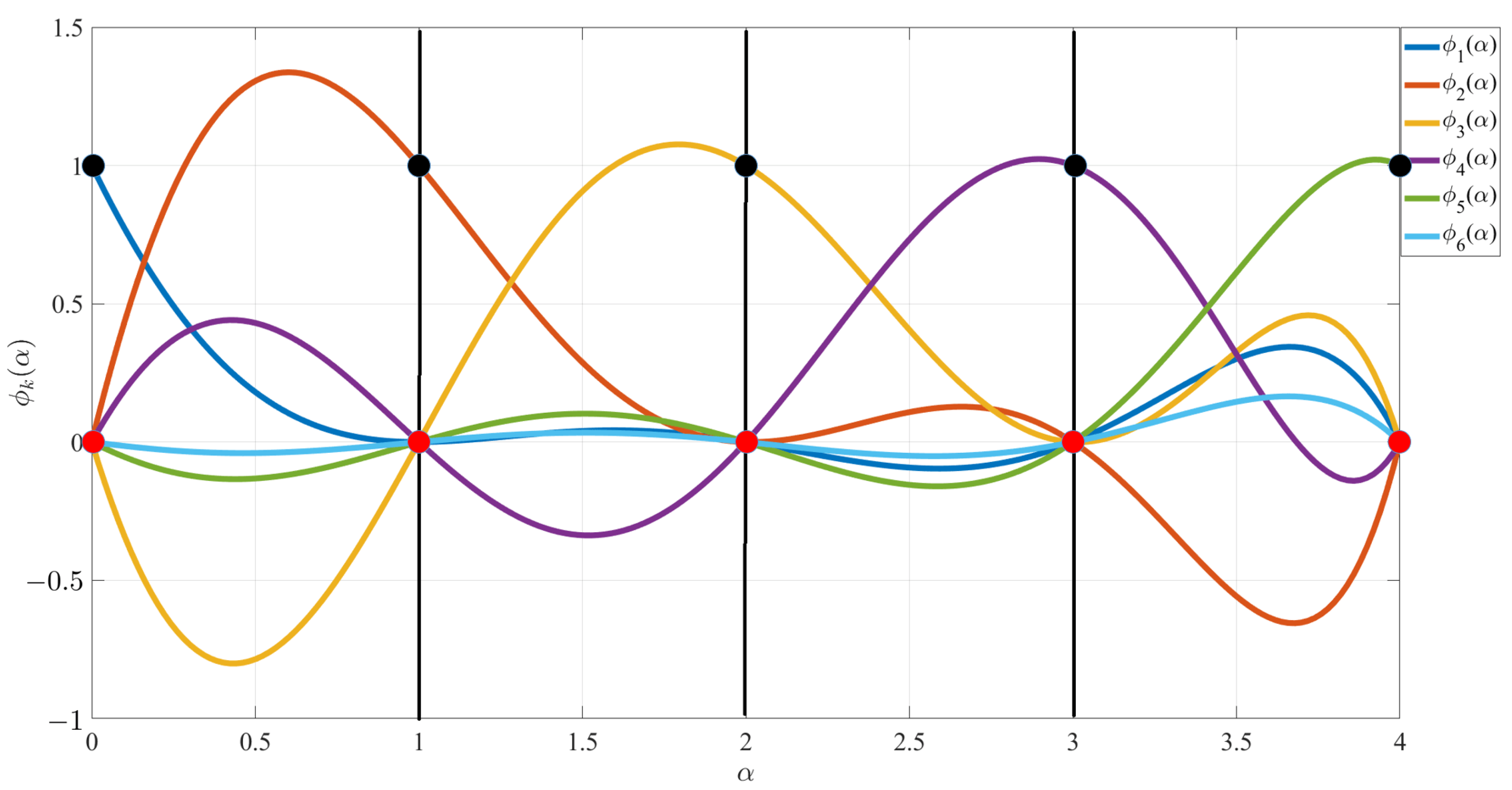
Since TFC can be applied to any integer and function sequences, the switching functions for natural numbers,
, play an important role for building functionals subject to integer derivatives and integrals. Note that the set of switching functions adopted for Equations (
8)–(
10) is the same.
To quantify the level of accuracy that can be obtained with this TFC approach, the following subsection provides a least-squares estimate of the free function to approximate the
function using Equation (
8).
3.3. Least-Squares Approximation of the Function
The function
is a continuous function interpolating the whole set of factorials
,
. The
function is not the only function that has this property. There are actually infinitely many ways to extend the factorials to a continuous function [
63], such as the Hadamard Gamma function
[
64], the logarithmic single-inflected factorial function
, and the logarithmic single-inflected hyper-factorial function
[
65]. However, it has been proved that the only function satisfying the recurrence relationship
for
is the
function [
66]. For this reason, the
function is rightfully considered the extension to reals of factorials. The recurrence property of Equation (
11) makes the
function the building block on which many existing fractional operators have been based.
Restricting the numerical interpolation example to the
range, a least-squares optimization problem has been solved using the constrained expression given in Equation (
8). This has been done by expressing
as a linear combination of 19 Legendre orthogonal polynomials (from
to
) since the polynomials from
to
are linearly dependent from the monomials used as support functions to derive the switching functions given in Equation (
6) and used to derive the constrained expression Equation (
8).
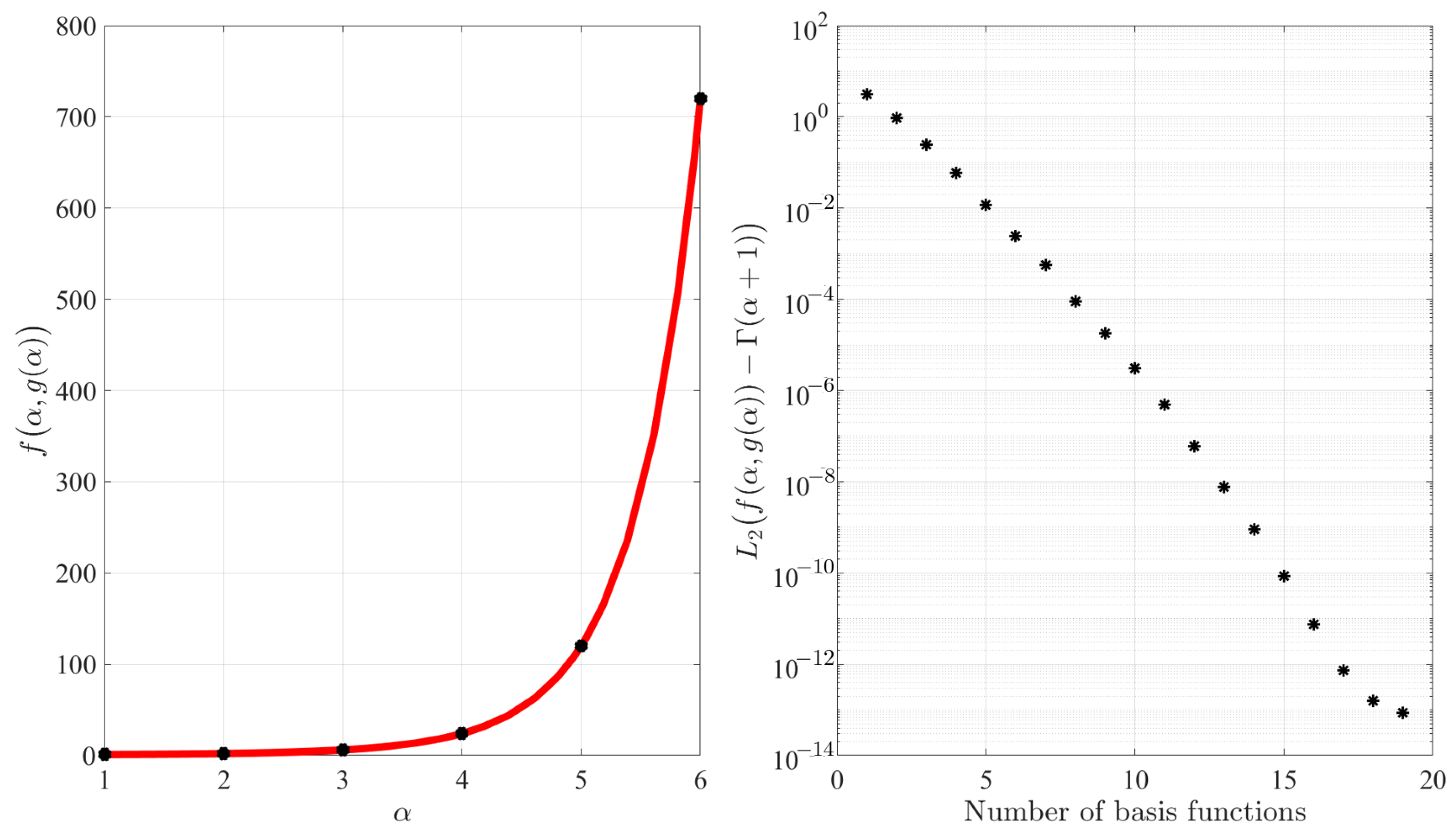
By discretizing the
range with
Chebyshev–Gauss–Lobatto points, the results of this approximation are given in
Figure 6. The left figure shows the resulting
function, while the right figure shows the
errors obtained in approximating the
function by increasing the number of basic functions adopted to expand the free function. Using 19 basis functions, the largest absolute error obtained (∼
) is close to the machine-error level with a condition number of the matrix to invert lower than 100, highlighting the robustness of this least-squares approximation.
It is important to highlight that obtaining a very good approximated expression of the function using polynomials allows easier further manipulations of it: for instance, manipulations requiring derivatives and/or integrals.
4. Least-Squares Approximation with Functional Interpolation
Performing a least-squares fitting of data provided by fractional operators presents a unique set of challenges. These operators, by their nature, are nonlocal, meaning they are defined over a specific range and not outside that range. This nonlocality and the selection of an initial point lead to the generation of boundary discontinuities at the domain bounds. For example, the Riemann–Liouville fractional operator definition requires the selection of an initial point, and the function is assumed to be constant before that point. This assumption generates a discontinuity at the selected point. This problem is partially solved in the Caputo definition by enforcing that the function is linear before the selected point. However, this entails a discontinuity at the same location. In the Grünwald–Letnikov formulation, a discontinuity arises from the truncation of an infinite series. The presence of discontinuities poses significant hurdles, precluding obtaining high accuracy in least-squares fitting problems using smooth functions.
Since fractional operators have continuity problems at the edges of the definition domain, the numerical validation of the proposed functional interpolation method to approximate fractional operators is numerically applied to the Mittag–Leffler function because this function is deeply adopted to derive fractional operators [
42], because it is a difficult function to compute (an infinite series expressed in terms of
functions), and because it was used to obtain closed-form expressions of Riemann–Liouville fractional derivatives and integrals of basic functions [
31], such as the exponential and the trigonometry functions.
Functional Approximation of the Mittag–Leffler Function
The Mittag–Leffler function appears in many areas of fractional calculus: for instance, in the fractional generalization of the heat equation, Lévy flights, superdiffusive transport, viscoelasticity, and random walks [
30]. The two-parameter Mittag–Leffler function [
30,
42] is
Setting
,
and using the surface notation, the one-parameter Mittag–Leffler function becomes [
29,
42]
One application of this function is to continuously morph between Gaussian and Lorentzian functions. Specifically, for
and
, the Mittag–Leffler function converges to
In addition, it is possible to prove that this function also satisfies
Equation (
12) represents two constraints at specific values of
a, while Equation (
13) represents two constraints at a specific value of
x. Using
as support functions, the recursive approach of multivariate TFC provides the functional that always satisfies the constraints given in Equation (
12):
while when using
as support functions, the functional always satisfying the constraints given in Equation (
13) is
The overall constrained expression is obtained by replacing the terms in
in Equation (
15) with the expressions of the corresponding terms
provided by Equation (
14). Removing all superscripts, the final constrained expression can be written in a compact way:
where
represents the surface interpolating the constraints given in Equations (
12) and (
13) using the support functions
and
, respectively, and
is the functional representing all surfaces that are not affecting the constraints (already satisfied by
): that is, representing all surfaces that are zeros at the constraints
as can be easily verified.
The free function is then estimated by least-squares by expanding it in terms of
n orthogonal surfaces,
, where
are the unknown coefficients of the expansion, and the orthogonal surfaces
are obtained using the product of Legendre’s orthogonal polynomials. The results of this optimization are shown in
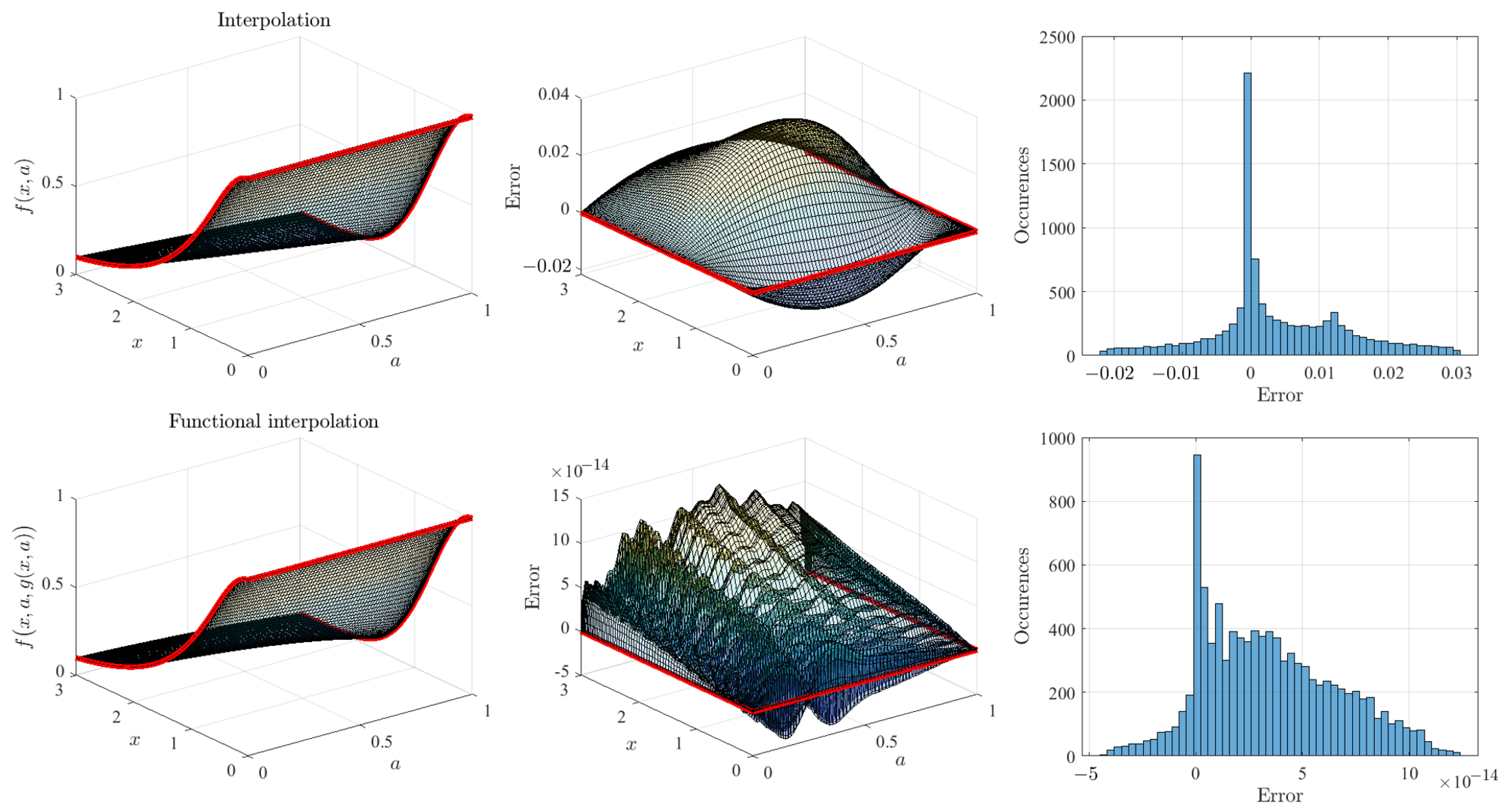
Figure 7.
The top-left plot of
Figure 7 shows the
surface: that is, the surface interpolating the constraints given by Equations (
12) and (
13) in the
domain. The difference between
and the Mittag–Leffler function (computed using the code provided in ref. [
67]) is given in the top-center figure and shows zero boundary errors (red lines). This error distribution is also provided by the histogram in the top-right figure, showing that the function
(simple interpolation) is accurate, with a maximum error lower than 0.03.
The bottom-left plot of
Figure 7 shows the surface obtained with Equation (
16), which is obtained by a linear least-squares estimation of the free function
. The fitting error of the Mittag–Leffler function is given in the bottom-center figure, while the error histogram is provided in the bottom-right figure. These last two plots outline the high accuracy obtained using just 35 orthogonal polynomials and discretizing the domain using
Chebyshev–Gauss–Lobatto points.
Expanding the free function using monomials (instead of orthogonal polynomials), the same optimization tests provided a maximum error lower than for the same domain discretization and 20 monomials. This approach can be applied to approximate any other continuous smooth complicated functions with boundary constraints. This example shows that these surfaces provide to the user various practical benefits/features: (1) highly accurate estimates, (2) functions are continuous (no need to interpolate between points), (3) computational complexity is low (requiring the evaluation of polynomials), (4) are local operators, and (5) they allow easier further manipulations (computing derivatives or integrals of polynomials is trivial).
5. Discussion
The geometrical meaning of fractional operators, derivatives, and integrals is still questionable. The existing proposed definitions are based on complicated integrals or infinite series that must be truncated to be used. In addition, these existing fractional operators are nonlocal, valid for specific domains, and/or require the selection of an initial point which, in turn, creates continuity issues.
Any proposed (past, present, and future) fractional operator definition has clear boundary constraints: it must provide the same expressions provided by the integer operators (whose geometrical meanings are clear). All different fractional operators, which are sometimes in contradiction with each other, are subject to these constraints. Based on this mandatory requirement, this article faces the fractional operators problem from an interpolation point of view by providing functionals representing all surfaces subject to the integer operator constraints when .
The interpolation problem is here performed using the theory of functional connections [
33,
34,
35,
36], an analytical theory providing functionals
representing all functions interpolating the mentioned integer constraints. The optimization is done by estimating (by least-squares) the expression of the free functions
. By doing this, the transitions between integer operators (derivatives and/or integrals) can be obtained as smooth continuous surfaces expressed in terms of polynomials.
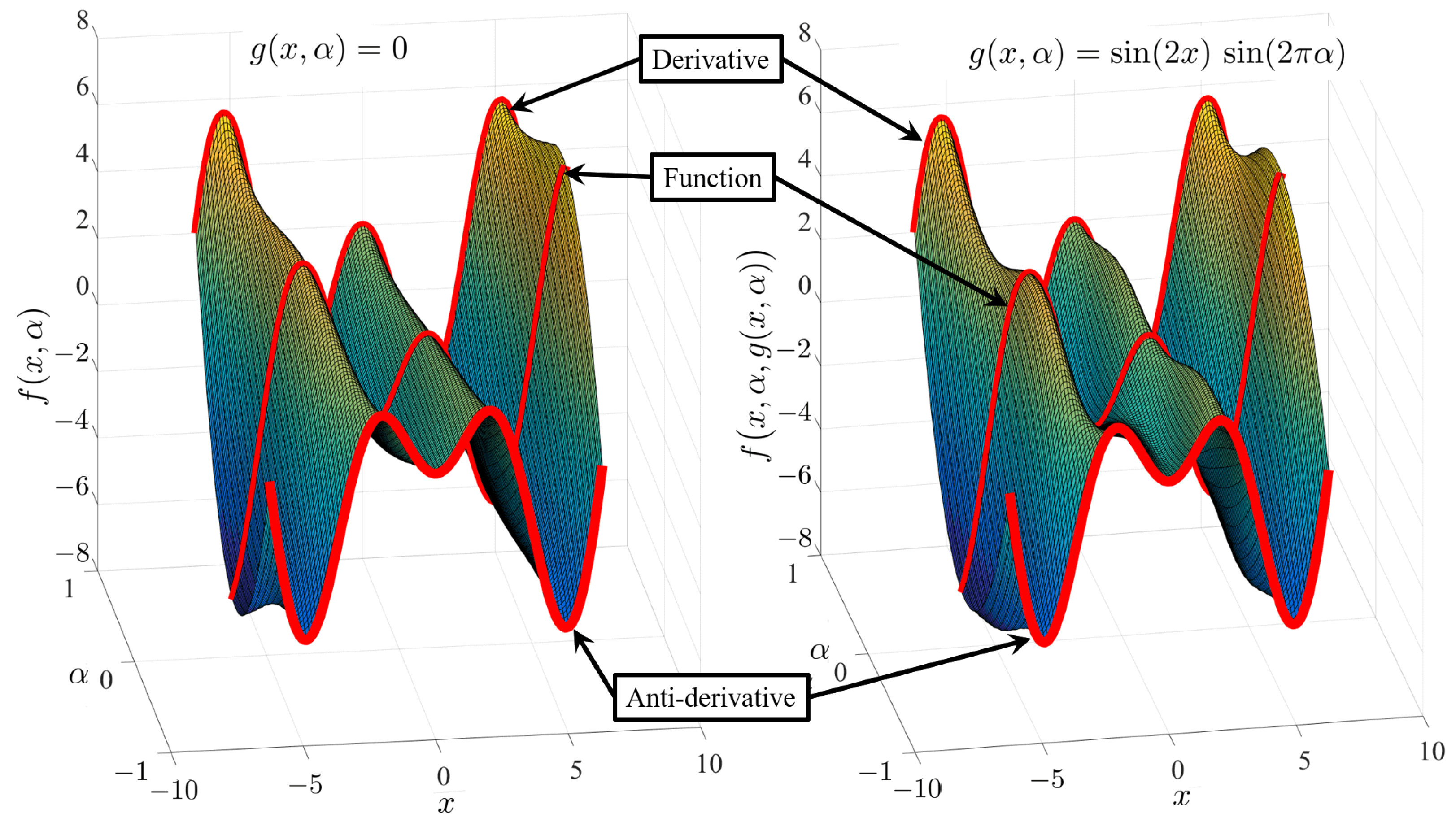
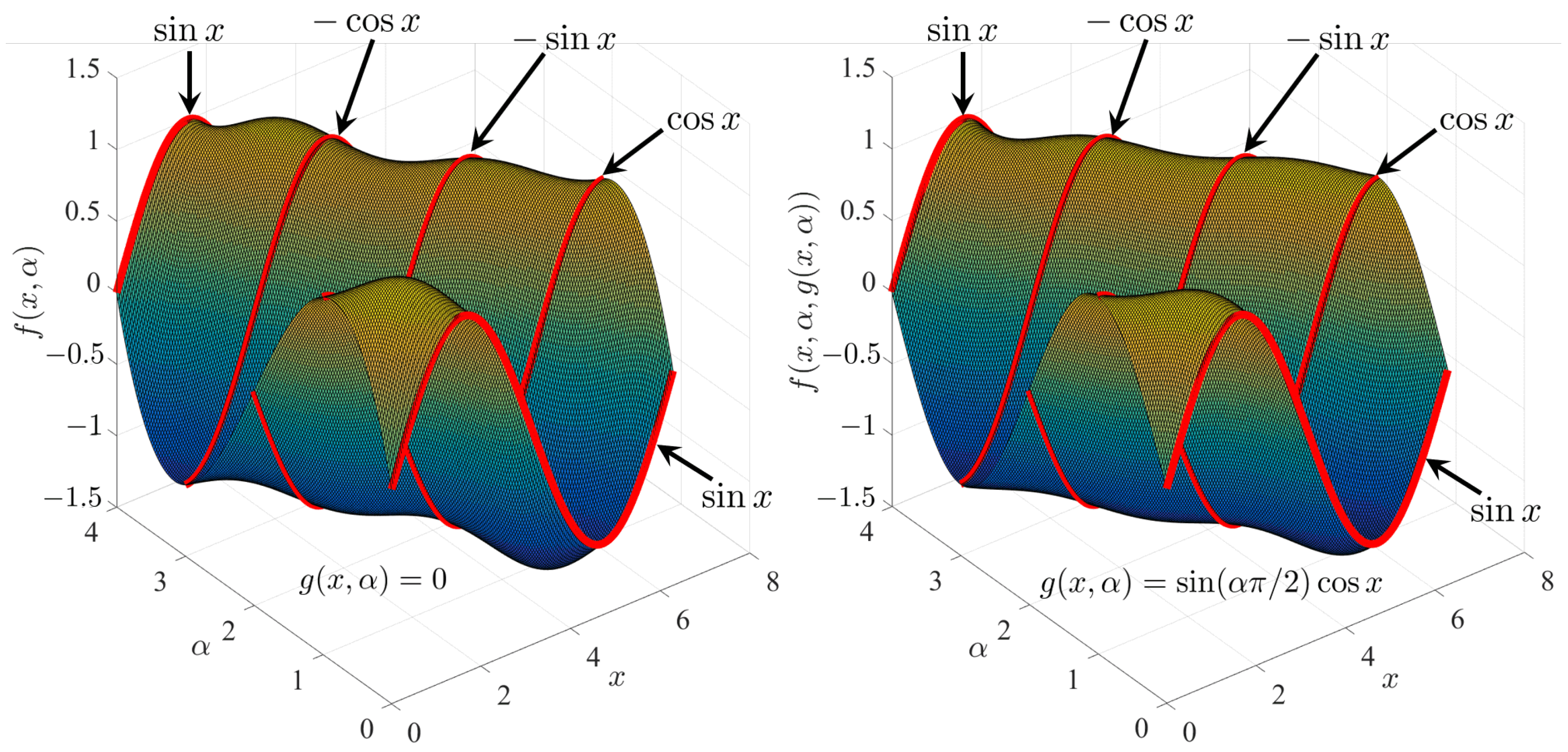
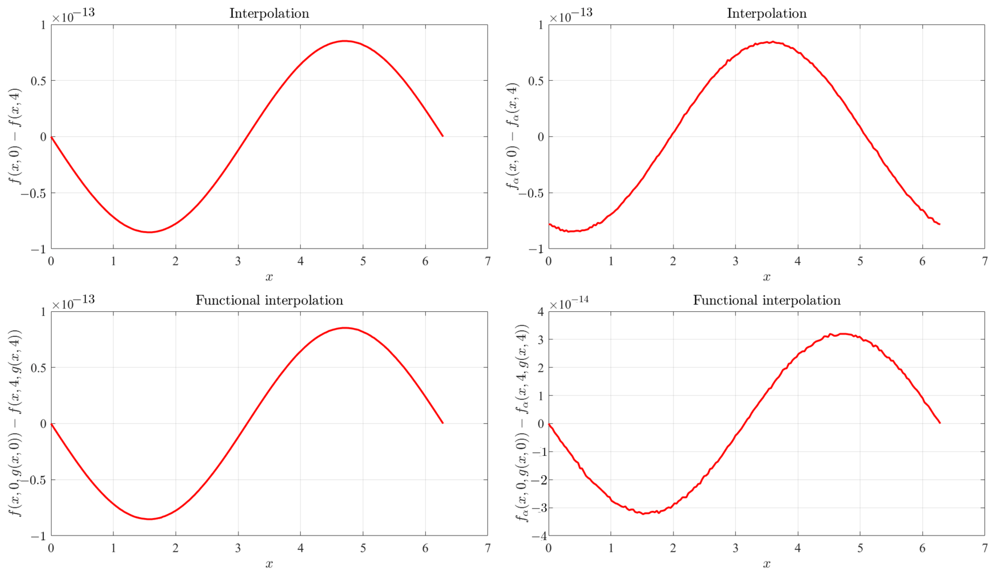
The flexibility of the proposed methodology has been shown by interpolating a function with its derivative and anti-derivative. This has been done using and with to show how the free function changes the surface while fully respecting the integer constraints. Another example shows the capability to derive all surfaces that are periodic in for the function . This means satisfying for any value of and for any expression of .
This article has also shown that functional interpolation can be used to obtain a continuous representation of any integer sequence (e.g., the Fibonacci sequence) and any function sequence (e.g., the Chebyshev orthogonal polynomials). For example, the function has been approximated at almost machine-error level with just a set of 19 Legendre orthogonal functions in the range . The closed-form expressions of the switching functions set for integer or function sequences have been derived. These expressions coincide with the fractional terms of the Lagrange polynomials.
The continuity issues affecting fractional operators at the selected initial point cause the function itself to lose the class of differentiability at that point. Because of this loss of smoothness, the least-squares fitting of fractional operator requires the adoption of non-smooth functions. Therefore, the numerical validation of the proposed approximation method has been tested on the Mittag–Leffler function; this was performed for additional reasons also [
31]. The resulting approximate expression of the Mittag–Leffle function is provided at almost machine-error level and with a limited number of orthogonal polynomials.
This functional interpolation method is general and can be applied to provide any transition surfaces between integer derivative and/or integral constraints. Once the optimization of the free function is estimated, then the resulting functional can be adopted as a smooth and accurate approximated local model of any fractional operator.


