Article

An Extended Gradient Method for Smooth and Strongly Convex Functions

1
School of Mathematics and Statistics, Xidian University, Xi’an 710126, China
2
School of Science, Chang’an University, Xi’an 710064, China
*
Authors to whom correspondence should be addressed.
Mathematics 2023, 11(23), 4771; https://doi.org/10.3390/math11234771
Submission received: 8 November 2023 / Revised: 22 November 2023 / Accepted: 24 November 2023 / Published: 26 November 2023
(This article belongs to the Section Computational and Applied Mathematics)

Abstract

:
In this work, we introduce an extended gradient method that employs the gradients of the preceding two iterates to construct the search direction for the purpose of solving the centralized and decentralized smooth and strongly convex functions. Additionally, we establish the linear convergence for iterate sequences in both the centralized and decentralized manners. Furthermore, the numerical experiments demonstrate that the centralized extended gradient method can achieve faster acceleration than the compared algorithms, and the search direction also exhibits the capability to improve the convergence of the existing algorithms in both two manners.

1. Introduction

In this work, we consider the unconstrained optimization problem:
min x R p f ( x ) .
The cost function f ( x ) : R p R of this problem is a differentiable strongly convex function, and the gradient f ( x ) is L-Lipschitz continuous. Starting from an initial point x 0 R p with f ( x 1 ) = 0 , the extended gradient method updates the iterates x k for k 0 :
x k + 1 = x k α ( f ( x k ) + f ( x k 1 ) ) ,
where the step size α ( α > 0 ) is sufficiently small, and it will be analyzed below to ensure the convergence of the extended gradient algorithm.
Firstly, we discussed briefly the accelerated scheme of gradient methods, that is, the iterate x k + 1 updates using the information of the preceding two iterates. Such as the gradient method with extrapolation that has the following forms: x k + 1 = x k α k f ( x k ) + β k ( x k x k 1 ) , where α k is the step size and β k [ 0 , 1 ) is a scalar. When α k and β k are set as the constant scalar α and β , respectively, the method is equivalent to the heavy ball method [1]. In [2], the linear convergence rate was established for the heavy ball method applied to smooth, twice continuously differentiable and strongly convex functions. Further, the authors in [3] constructed an example to illustrate that even if the objective functions are strongly convex, the heavy ball method still can not converge when the functions are not twice continuously differentiable. Thus, the property that the objective function is twice continuously differentiable is a necessary condition in the convergence guarantees of the heavy ball method. Based on this fact, for the case of strictly convex quadratic functions, the recent work [4], obtained the iteration complexity of the heavy ball method under the assumption that the appropriate upper and lower bounds for eigenvalues of the Hessian matrix are known. In particular, several accelerated gradient descent methods with a similar structure to the heavy ball method also have been proposed in [5], and they converge linearly to the solution of the smooth and strongly convex functions with the optimal iteration complexity. Compared to the heavy ball method, the above accelerated methods fully utilize the difference between the preceding two iterates. Moreover, the main advantage of solving convex functions in practice is that the accelerated gradient descent methods can converge to the optimum more quickly [6].
On the other hand, the accelerated scheme also can update the variables employing the gradients of the preceding several iterates. As mentioned in [7,8], the optimistic gradient descent-ascent (OGDA) method and the inertial gradient algorithm with Hessian dampling (IGAHD) update the variable via the difference of the gradients of the preceding two iterates. Besides, for the least mean squares (LMS) estimation of graph signals, the extended LMS algorithm in [9] and proportionate-type graph LMS algorithm in [10] update the variable via the weighted sum of the gradients of the preceding several iterates. Further, the Anderson acceleration gradient descent method (AA-PGA) in [11] updates the variable by employing the convex combination of the gradients of the preceding several iterates. However, AA-PGA converges linearly to the optimal solution x * under the assumption 2 f ( x * ) υ I . Inspired by the above works, we here introduce an extended gradient method, in which the variables are updated along the direction of the sum of the gradients of the preceding two iterates. The main purpose of this work is to analyze the convergence of the extended gradient method for finding the optimal solution of problem (1). We will show that when the step size is less than a given upper bound, the linear convergence of the extended gradient method can be guaranteed.
Next, we consider a class of smooth and strongly convex optimization functions on the real vector space with Euclidean norm · and inner product · , · .
Definition 1.
A function f : R p R is L-smooth if the gradient f ( x ) is L-Lipschitz continuous, that is,
f ( x ) f ( y ) L x y , x , y .
If f is convex and L-smooth it also holds that f ( x ) f ( y ) + f ( y ) , x y + L 2 x y 2 [12].
Definition 2.
A function f : R p R is μ-strongly convex if there exists μ > 0 such that
f ( x ) f ( y ) + f ( y ) , x y + μ 2 x y 2 .

2. Analysis of the Extended Gradient Method

In this section, to establish the convergence of the extended gradient method, we first obtain an important inequality in Theorem 1, where the upper bound on x k + 1 x * will be given in terms of the linear combinations of x k x * , x k 1 x * and x k 2 x * . This inequality is vital and will be used in the following analysis.
Theorem 1.
Assume that f is μ-strongly convex, and the gradient f ( x ) is L-Lipschitz continuous. Let the step size α satisfy the condition 0 α 1 + 2 μ L 1 2 L , and { x k } k N be generated by the extended gradient method (2). Then, the following hold.
(i) The iterates { x k } satisfy the following linear inequality
x k + 1 x * 2 ( 1 + 2 α 2 L 2 α μ ) x k x * 2 + ( 2 α 2 L 2 + 2 α 3 L 3 α μ ) x k 1 x * 2 + 2 α 3 L 3 x k 2 x * 2 ,
where x * is the optimal solution.
(ii) min 2 k K f ( x k )  converges to the optimal value f ( x * ) at the sub-linear rate of O ( 1 K ) .
Proof. 
(i) According to the update equation in (2), for any x R p , we have
x k + 1 x 2 = x k α ( f ( x k ) + f ( x k 1 ) ) x 2 = x k x 2 + α 2 f ( x k ) + f ( x k 1 ) 2 2 α ( f ( x k ) + f ( x k 1 ) ) T ( x k x ) = x k x 2 + α 2 Γ 1 2 α ( Γ 2 + Γ 3 ) ,
where Γ 1 : = f ( x k ) + f ( x k 1 ) 2 , Γ 2 : = f ( x k ) T ( x k x ) , and Γ 3 : = f ( x k 1 ) T ( x k x ) .
Now, substituting x = x * , and noting that f ( x * ) = 0 , we first bound the term Γ 1 ,
Γ 1 2 f ( x k ) 2 + 2 f ( x k 1 ) 2 = 2 f ( x k ) f ( x * ) 2 + 2 f ( x k 1 ) f ( x * ) 2 2 L 2 x k x * 2 + 2 L 2 x k 1 x * 2 .
Secondly, we provide a lower bound of Γ 2 with the strongly convex property of f ( x ) ,
Γ 2 = f ( x k ) T ( x k x * ) f ( x k ) f ( x * ) + μ 2 x k x * 2 .
Finally, we bound the term Γ 3 by employing Γ 1 and Γ 2 . Based on the smoothness of f, we can obtain that
f ( x k ) f ( x k 1 ) + f ( x k 1 ) T ( x k x k 1 ) + L 2 x k x k 1 2 .
Add and subtract the inner product f ( x k 1 ) T x * to the right-hand side of (6) and rearrange the terms to have
f ( x k ) f ( x k 1 ) + f ( x k 1 ) T ( x * x k 1 ) + L 2 x k x k 1 2 + f ( x k 1 ) T ( x k x * ) .
Then by the bound of Γ 2 (5) (k is replaced by k 1 ), (7) can be rewritten as
f ( x k ) f ( x * ) μ 2 x k 1 x * 2 + L 2 x k x k 1 2 + f ( x k 1 ) T ( x k x * ) ,
wherein, in terms of the update Equation (2) and the bound of Γ 1 (4), the term x k x k 1 2 in (8) can be further expressed as
x k x k 1 2 = α 2 f ( x k 1 ) + f ( x k 2 ) 2 2 α 2 L 2 x k 1 x * 2 + 2 α 2 L 2 x k 2 x * 2 .
Therefore, the bound of Γ 3 can be yielded as
Γ 3 = f ( x k 1 ) T ( x k x * ) f ( x k ) f ( x * ) + ( μ 2 α 2 L 3 ) x k 1 x * 2 α 2 L 3 x k 2 x * 2
Substituting (4), (5) and (10) (the bounds of Γ 1 , Γ 2 , and Γ 3 ) into (3), we have
x k + 1 x * 2 ( 1 + 2 α 2 L 2 α μ ) x k x * 2 + ( 2 α 2 L 2 + 2 α 3 L 3 α μ ) x k 1 x * 2 + 2 α 3 L 3 x k 2 x * 2 4 α ( f ( x k ) f ( x * ) ) .
Considering that f ( x k ) f ( x * ) in (11), we complete the proof of (i).
(ii) Rearranging the terms in (11), it holds
4 α ( f ( x k ) f ( x * ) ) x k x * 2 x k + 1 x * 2 2 α 3 L 3 x k 1 x * 2 x k 2 x * 2 + ( 2 α 2 L 2 α μ ) x k x * 2 + ( 2 α 2 L 2 + 4 α 3 L 3 α μ ) x k 1 x * 2 .
For 0 α 1 + 2 μ L 1 2 L , we obtain 2 α 2 L 2 + 4 α 3 L 3 α μ ( 2 α 2 L 2 α μ ) and thus
4 α ( f ( x k ) f ( x * ) ) x k x * 2 x k + 1 x * 2 2 α 3 L 3 x k 1 x * 2 x k 2 x * 2 ( 2 α 2 L 2 α μ ) ( x k 1 x * 2 x k x * 2 ) .
Summing over k = 2 , , K , we have
k = 2 K 4 α f ( x k ) f ( x * ) x 2 x * 2 x K + 1 x * 2 2 α 3 L 3 ( x K 1 x * 2 x 0 x * 2 ) ( 2 α 2 L 2 α μ ) ( x 1 x * 2 x K x * 2 ) .
Noticed that 0 α 1 + 2 μ L 1 2 L μ 2 L 2 , then ( 2 α 2 L 2 α μ ) x K x * 2 < 0 . Therefore, the following inequality holds
min 2 k K f ( x k ) f ( x * ) x 2 x * 2 ( 2 α 2 L 2 α μ ) x 1 x * 2 + 2 α 3 L 3 x 0 x * 2 4 α ( K 2 ) ,
which means that min 2 k K f ( x k )  converges to the optimal value f ( x * ) at the sub-linear rate of O ( 1 K ) . □
The result in (ii) of Theorem 1 shows that the function value generated by the extended gradient method converges to the optimal solution of problem (1) at a sublinear rate. Further, in order to derive the linear convergence of the extended gradient method, we give two important lemmas as follows.
Lemma 1
([13] Corollary 8.1.29). Let A R n × n be a nonnegative matrix, and ω R n be a positive vector. If A ω < q ω , then ρ ( A ) < q .
Lemma 2
([14] Lemma 1 in Section 2.1). It holds that ρ ( A ) = lim k A k 1 k , i.e., the spectral radius of A gives the asymptotic growth rate of A k : For every ϵ > 0 there is c = c ( ε ) such that A k c ( ρ ( A ) + ε ) k , for all k.
Together with (i) of Theorem 1, Lemma 1 and Lemma 2, we give the following Theorem 2. For notational convenience, we define z k : = ( x k x * 2 , x k 1 x * 2 , x k 2 x * 2 ) .
Theorem 2.
The same assumptions hold as in Theorem 1. Let the sequence { x k } generated by the extended gradient method and x * be the optimal solution. Then for every ε > 0 , there is c = c ( ϵ ) such that || z k + 1 || c ( ρ ( A ) + ϵ ) k z 0 , for all k, where ρ ( A ) < 1 is a constant.
Proof. 
By the result in (i) of Theorem 1, we first readily find that z k + 1 A z k , here A = 1 + 2 α 2 L 2 α μ 2 α 2 L 2 + 2 α 3 L 3 α μ 2 α 3 L 3 1 0 0 0 1 0 .
Under the assumption that the spectral radius of matrix A is less than 1 (i.e., ρ ( A ) < 1 ), the statement of convergence can be obtained via Lemma 2. Thus, it remains to analyze the spectral radius of the matrix A and show that the spectral radius of A is less than 1. Find a positive vector c = [ c 1 , c 2 , c 3 ] T satisfying A c < c , then the following inequalities hold
( 2 α 2 L 2 α μ ) c 1 + ( 2 α 2 L 2 + 2 α 3 L 3 α μ ) c 2 + 2 α 3 L 3 c 3 < 0 ; c 1 < c 2 ; c 2 < c 3 .
To ensure that the first inequality in (16) holds, the necessary condition is that 2 α 2 L 2 α μ < 0 , which means α < μ 2 L 2 . Then, according to the sign of 2 α 2 L 2 + 2 α 3 L 3 α μ , we further deduce the bounds of α by considering the following two cases.
(i) If 2 α 2 L 2 + 2 α 3 L 3 α μ > 0 , we can derive the first inequality of (16) as
( 2 α 2 L 2 α μ ) c 1 + ( 2 α 2 L 2 + 2 α 3 L 3 α μ ) c 2 + 2 α 3 L 3 c 3 > ( 4 α 2 L 2 + 2 α 3 L 3 2 α μ ) c 1 + 2 α 3 L 3 c 3 ,
duo to 0 < c 1 < c 2 . Then, since the left-hand side of the (17) is less than 0, we have
2 α 3 L 3 c 3 < ( 4 α 2 L 2 + 2 α 3 L 3 2 α μ ) c 1 < ( 4 α 2 L 2 + 2 α 3 L 3 2 α μ ) c 3 ,
due to 0 < c 1 < c 3 . Further, it follows from (18) that ( 4 α 2 L 2 + 2 α 3 L 3 2 α μ ) c 3 2 α 3 L 3 c 3 > 0 , namely, 2 α 2 L 2 + 2 α 3 L 3 α μ < 0 , which leads to a contradiction to the assumption.
(ii) If 2 α 2 L 2 + 2 α 3 L 3 α μ 0 , the first inequality of (16) can be written as
( 2 α 2 L 2 α μ ) c 1 + ( 2 α 2 L 2 + 2 α 3 L 3 α μ ) c 2 + 2 α 3 L 3 c 3 > ( 2 α 2 L 2 α μ ) c 1 + ( 2 α 2 L 2 + 4 α 3 L 3 α μ ) c 3 ,
due to 0 < c 2 < c 3 . Then, based on the fact that the left-hand side of (19) is less than 0, we have
( 2 α 2 L 2 + 4 α 3 L 3 α μ ) c 3 < ( 2 α 2 L 2 α μ ) c 1 < ( 2 α 2 L 2 α μ ) c 3 ,
due to 0 < c 1 < c 3 . On rearranging the terms of (20), we obtain that 2 ( 2 α 2 L 2 + 2 α 3 L 3 α μ ) c 3 < 0 , which is consistent with the assumption. Therefore, the upper bound of step size α can be reduced as
α < 1 + 2 μ L 1 2 L = min μ 2 L 2 , 1 + 2 μ L 1 2 L .
Finally, we have demonstrated that there exists a positive vector c = [ c 1 , c 2 , c 3 ] T such that A c < c , then it is clear ρ ( A ) < 1 according to Lemma 1 for a < 1 + 2 μ L 1 2 L . □
Remark 1.
Choose α min { 1 6 L , 1 + 2 μ L 1 2 L } and assume that f ( x k 2 ) 2 f ( x k 1 ) for some fix k. It follows that
f ( x k 1 ) f ( x k ) f ( x k 1 ) + f ( x k ) L x k x k 1 + f ( x k ) = L α f ( x k 1 ) + f ( x k 2 ) + f ( x k ) L α f ( x k 1 ) + f ( x k 2 ) + f ( x k ) 3 L α f ( x k 1 ) + f ( x k ) 1 2 f ( x k 1 ) + f ( x k ) ,
which means that f ( x k 1 ) 2 f ( x k ) . By induction and by the selections of initial points, it can be ensured that f ( x k 1 ) 2 f ( x k ) for all k N . As a consequence, by defining g k : = f ( x k ) + f ( x k 1 ) , we obtain g k f ( x k ) 2 f ( x k ) . This is indeed similar to the inexact condition considered in [14] (Theorem 2 in Section 4.2.3), [15,16]. Note, that [14] considers the methods of the form
x k + 1 = x k α k g k , w h e r e g k f ( x k ) η f ( x k ) ,
and where η ( 0 , 1 ) for the convex functions with Lipschitz continuous gradients. While [15,16] considers the methods of type ( 0 , 2 3 ) for smooth functions without convexity. The constant 2 in the extended gradient method can relax the inexact condition.

3. Analysis of the Decentralized Extended Gradient Method

The traditional (centralized) optimization methods are found on a large assumption that all data samples are stored and operated at a computing unit [17]. However, in the networked multi-agent systems, the data resources and function information related to optimization problems are stored in each agent distribution, and the distributed schemes are introduced into the framework of optimization [18]. In the distributed fashion, all data are transmitted to a fusion center that conducts the optimization operation and scatters the updated information to all agents. Nevertheless, the distributed operation is gradually replaced by the decentralized manner for the reasons of privacy and communication costs. The decentralized optimization is designed for the situations of networked systems which can fully utilize the resources of multiple computing units and improve the reliability of the networked systems.
In this section, we focus on distributed gradient methods. The earlier distributed gradient methods [19,20,21] slowly converge to the optimal solution by utilizing the diminishing step size. With the constant step size, these methods only converge to a neighborhood of the optimal solution. Recently, the distributed gradient methods [22,23,24] combined with more techniques can converge linearly to the optimal solution. The techniques include the multi-step consensus, the difference between the two consecutive iterates and the gradient tracking technique, which could cause more computation and communication burden. Thus, we try to investigate the behavior of the decentralized extended gradient method working with the simple update mechanism.

3.1. Decentralized Extended Gradient Method

This section develops a decentralized version of the extended gradient method for the following problem:
min x R p f ( x ) = 1 n i = 1 n f i ( x ) ,
where the local cost function f i is L-smooth and μ -strongly convex, which is defined over a network consisting of n agents. To apply the extended gradient method to problem (22) under the decentralized situation, all the agents carry out the extended gradient method in parallel.
A set of local variables { x i R p } i = 1 n is introduced, and x i is assigned to agent i. Denote the aggregate variable X and the aggregate gradient F ( X ) as X = ( x 1 , x 2 , , x n ) and F ( X ) = ( f 1 ( x 1 ) , f 2 ( x 2 ) , , f n ( x n ) ) . The decentralized extended gradient method updates the iterates X k + 1 :
X k + 1 = W X k α ( F ( X K ) + F ( X k 1 ) ) ,
where the weight matrix W is symmetric and double stochastic, i.e., W = W , W 1 n = 1 n and 1 n W = 1 n , herein 1 n = ( 1 , , 1 ) R p . Weight the matrix W is generated based on the network. When the agent i and j are neighbors or i = j , W i j 0 . In the decentralized setting, the local function f i is only accessed by agent i, i = 1 , , n . All agents cooperate to optimize the global function f via local intra-node computation and extra-node communication. The local computation is operated on the individual agent, i.e., the local variable of agent i is updated by the gradient information of the local function f i . The communication is operated over the network, i.e., the local variable is updated by combining the weighted average of its neighbor’s local variable, which enforces the consensus of all local variables.

3.2. Convergence Result

We need to define the average vector: X ¯ k = 1 n 1 n X k = 1 n i = 1 n x i k R 1 × p . Then, we give the upper bounds on X ¯ k ( x * ) and X k 1 n X ¯ k by using the linear combinations of the values of the preceding two iterates.
Lemma 3.
Let { X k } k N be the iterates generated by the updates in (23). If ξ ( α 1 ( n 1 ) α , α + 1 ( n 1 ) α ) , then the following relation hold:
z k + 1 A z k ,
where z k = X k 1 n X ¯ k , X ¯ k ( x * ) , X k 1 1 n X ¯ k 1 , X ¯ k 1 ( x * ) R 4 and  A = δ + ξ L α n 1 α ( ξ 2 2 α ξ + n α 2 ) ξ L α n ( n 1 ) α ( ξ 2 2 α ξ + n α 2 ) ξ L α n 1 α ( ξ 2 2 α ξ + n α 2 ) ξ L α n ( n 1 ) α ( ξ 2 2 α ξ + n α 2 ) α L n λ α L n α L 1 0 0 0 0 1 0 0 R 4 × 4 , here in λ = max { | 1 α L | , | 1 α μ | } and δ = W 1 n 1 n n .
If 1 μ + L < α < min { 2 L , n γ 2 L ( γ 1 + n γ 2 + γ 3 + n γ 4 ) } and ξ ( α 1 ( n 1 ) α , min { α + 1 ( n 1 ) α , b 2 4 a c 2 a } ) , where 0 < γ 1 < γ 3 , 0 < γ 2 < γ 4 , a = ( 1 δ ) γ 1 , b = α L n 1 ( γ 1 + n γ 2 + γ 3 + n γ 4 ) + 2 ( 1 δ ) α γ 1 and c = ( 1 δ ) ( n α 2 α ) , then ρ ( A ) < 1 and thus X k 1 n X ¯ k and X ¯ k ( x * ) converge to zero at the linear rate of O ( ρ ( A ) k ) .
Proof. 
First, we establish a linear system by using the upper bounds on X k + 1 1 n X ¯ k + 1 and X ¯ k + 1 ( x * ) . Next, we can find the range of α such that ρ ( A ) < 1 . From the update in (23), we derive
X ¯ k + 1 = 1 n 1 n W X k α F ( X k ) + F ( X k 1 ) = X ¯ k α n 1 n F ( X k ) + F ( X k 1 ) .
Step 1. Bound X k + 1 1 n X ¯ k + 1 .
From the above equation, it follows that
X k + 1 1 n X ¯ k + 1 = ( I 1 n 1 n 1 n ) ( W X k α ( F ( X K ) + F ( X k 1 ) ) ) ( I 1 n 1 n 1 n ) W X k + I 1 n 1 n 1 n α F ( X K ) + α F ( X k 1 )
Notice that I 1 n 1 n 1 n W = W 1 n 1 n 1 n I 1 n 1 n 1 n and I 1 n 1 n 1 n = n 1 . Therefore, it follows
X k + 1 1 n X ¯ k + 1 δ X k 1 n X ¯ k + n 1 α F ( X k ) + α F ( X k 1 ) ,
where δ = W 1 n 1 n 1 n < 1 . For the term α F ( X k ) , we can further bound as
α F ( X k ) = α F ( X k ) ξ n 1 n 1 n F ( X k ) + ξ n 1 n 1 n F ( X k ) ξ 1 n f ( X ¯ k ) + ξ 1 n f ( X ¯ k ) ξ 1 n f ( x * ) ( α I ξ n 1 n 1 n ) F ( X k ) + ξ 1 n 1 n i = 1 n f i ( x i k ) f i ( X ¯ k ) + ξ 1 n 1 n i = 1 n f i ( X ¯ k ) f i ( x * ) α I ξ n 1 n 1 n F ( X k ) + ξ 1 n 1 n i = 1 n f i ( x i k ) f i ( X ¯ k ) + ξ 1 n 1 n i = 1 n f i ( X ¯ k ) f i ( x * ) ( ξ 2 2 α ξ + n α 2 ) F ( X k ) + ξ n 1 n i = 1 n f i ( x i k ) f i ( X ¯ k ) + ξ n 1 n i = 1 n f i ( X ¯ k ) f i ( x * ) ( ξ 2 2 α ξ + n α 2 ) F ( X k ) + ξ L n 1 n i = 1 n x i k X ¯ k + ξ L n X ¯ k ( x * ) ( ξ 2 2 α ξ + n α 2 ) F ( X k ) + ξ L n i = 1 n x i k X ¯ k 2 n + ξ L n X ¯ k ( x * ) ( ξ 2 2 α ξ + n α 2 ) F ( X k ) + ξ L X k 1 n X ¯ k + ξ L n X ¯ k ( x * ) ,
where choosing ξ ( α 1 ( n 1 ) α , α + 1 ( n 1 ) α ) such that α ( ξ 2 2 α ξ + n α 2 ) > 0 . So
F ( X k ) 1 α ( ξ 2 2 α ξ + n α 2 ) ( ξ L X k 1 n X ¯ k + ξ L n X ¯ k ( x * ) ) .
Similarly, we have
F ( X k 1 ) 1 α ( ξ 2 2 α ξ + n α 2 ) ( ξ L X k 1 1 n X ¯ k 1 + ξ L n X ¯ k 1 ( x * ) ) .
Substituting (28) and (29) into (26) yields
X k + 1 1 n X ¯ k + 1 ( δ + ξ L α n 1 α ( ξ 2 2 α ξ + n α 2 ) ) X k 1 n X ¯ k + ξ L α n ( n 1 ) α ( ξ 2 2 α ξ + n α 2 ) X ¯ k ( x * ) + ξ L α n 1 α ( ξ 2 2 α ξ + n α 2 ) X k 1 1 n X ¯ k 1 + ξ L α n ( n 1 ) α ( ξ 2 2 α ξ + n α 2 ) X ¯ k 1 ( x * ) .
Step 2. Bound X ¯ ( x * ) .
X ¯ k + 1 ( x * ) = X ¯ k α 1 n n ( F ( X k ) + F ( X k 1 ) ) ( x * ) = X ¯ k α 1 n n F ( 1 n X ¯ k ) ( x * ) + α 1 n n ( F ( 1 n X ¯ k ) F ( X k ) ) α 1 n n F ( X k 1 ) X ¯ k α f ( X ¯ k ) ( x * ) + α 1 n n ( F ( 1 n X ¯ k ) F ( X k ) ) + α 1 n n F ( X k 1 ) .
Consider the first term in (31), we have
X ¯ k α f ( X ¯ k ) ( x * ) λ X ¯ k ( x * ) ,
where λ = max { | 1 α L | , | 1 α μ | } . For the second term and third term in (31), we bound them as
1 n n ( F ( 1 n X ¯ k ) F ( X k ) ) L n X k 1 n X ¯ k .
and
1 n n F ( X k 1 ) = 1 n n F ( X k 1 ) 1 n n F ( 1 n X ¯ k 1 ) + 1 n n F ( 1 n X ¯ k 1 ) 1 n n F ( 1 n ( x * ) ) L n X k 1 1 n X ¯ k 1 + L X ¯ k 1 ( x * ) ,
due to the smoothness of global function f. Substituting (32)–(34) into (31), it holds
X ¯ k + 1 ( x * ) L α n X k 1 n X ¯ k + λ X ¯ k ( x * ) + L α n X k 1 1 n X ¯ k 1 + L α X ¯ k 1 ( x * ) .
The linear system in (24) is obtained by using the results of (30) and (35).
Next, According to Lemma 1, we give the range of α and ξ and a positive vector γ = ( γ 1 , γ 2 , γ 3 , γ 4 ) such that A γ < γ , which is equivalent to the following inequalities
ξ L α n 1 γ 1 + ξ L α n ( n 1 ) γ 2 + ξ L α n 1 γ 3 + ξ L α n ( n 1 ) γ 4 < ( 1 δ ) ( α ( ξ 2 2 α ξ + n α 2 ) ) γ 1 ,
L α n γ 1 + L α n γ 3 + α L γ 4 < ( 1 λ ) γ 2 ,
γ 1 < γ 3 ,
γ 2 < γ 4 .
If 1 L + μ < α < 2 L , according to the definition that λ = max { | 1 α μ | , | 1 α L | } , we have that l λ = 2 α L > 0 . Since α satisfies (37), we require
1 μ + L < α < min { 2 L , n γ 2 L ( γ 1 + n γ 2 + γ 3 + n γ 4 ) }
The range of ξ follows (36), that is,
ξ ( α 1 ( n 1 ) α , min { α + 1 ( n 1 ) α , b 2 4 a c 2 a } ) ,
where a = ( 1 δ ) γ 1 , b = α L n 1 ( γ 1 + n γ 2 + γ 3 + n γ 4 ) + 2 ( 1 δ ) α γ 1 and c = ( 1 δ ) ( n α 2 α ) . Then, consider that γ 1 , γ 2 , γ 3 and γ 4 are positive, we can select proper γ 1 , γ 2 , γ 3 ( > γ 1 ) and γ 4 ( > γ 2 ) to make the set in (41) be nonempty. □

4. Numerical Experiments

In this section, we perform computational experiments on both the centralized and the decentralized problems to demonstrate the efficiency of the extended gradient method. We compare our proposed method with many well-known algorithms. All algorithms are programmed in Matlab (R2018b, MathWorks, Natick, MA, USA) and run on a PC (Lenovo-M430, Beijing, China) with a 2.90 GHz Intel Core i5-10400 CPU and 8 GB of memory.

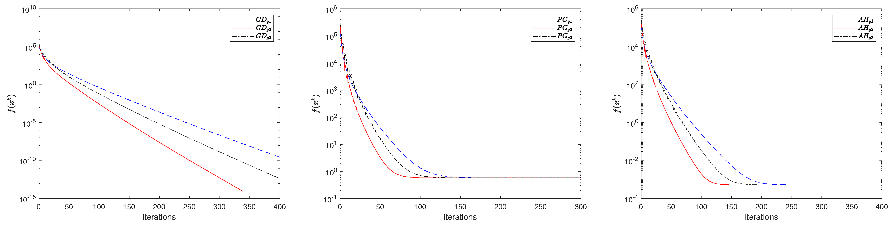
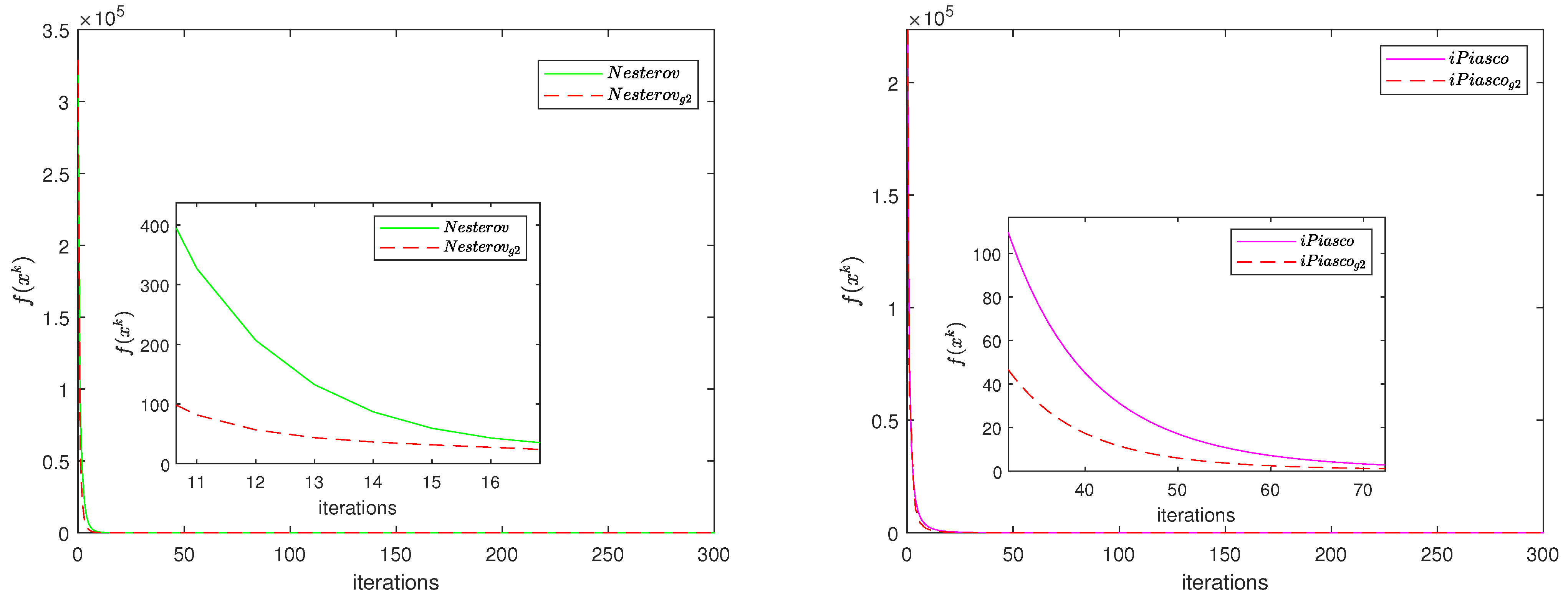
4.1. Centralized Problem

We consider the performance of the extended gradient method when it is applied to the LASSO problem:
min x R p f ( x ) = 1 2 M x b 2 + ν x 1 ,
where the random matrix M R m × p is generated by the uniform distribution U ( 0 , 1 ) , b = M x where x also follows an uniform distribution U ( 0 , 1 ) with sparsity r. In particular, we set the parameters m = 512 , p = 1024 , r = 0.1 , and the initial condition x 0 U ( 0 , 1 ) . The termination criterion is set to reach the maximum number of iterations or | f ( x k ) f ( x k 1 ) | 10 15 . When the regularization parameter ν is zero, the LASSO problem becomes the least squares problem. Otherwise, the objective function f ( x ) is nonsmooth. Considering that the nonsmooth term x 1 is actually the sum of the absolute values of each component of x, we employ the proximal gradient method and the approximation method based on the Huber function, respectively, to solve the LASSO problem. The Huber function becomes closer to the absolute value function as the parameter θ approaches 0.
h θ = 1 2 θ x 2 , | x i | < θ | x i | θ 2 , o t h e r w i s e
In order to study the influence of the previous gradients on the search direction of the optimization algorithm, we employ the gradient (denoted as g 1 ), the sum of the gradients of the preceding two iterates (denoted as g 2 ), and the sum of the gradients of the preceding three iterates (denoted as g 3 ) to construct search directions, respectively. Figure 1 shows the performance of the gradient descent method(GD) for the least square problem, the proximal gradient method(PG) and the approximation method based on the Huber function (AH) for the LASSO problem ( ν = 0.001 ) when the above three search directions are employed. We set the parameter θ as 0.02. For these algorithms with the three search directions, we set the step sizes as 1 L , 0.8 1 L and 0.4 1 L , respectively. Observing that when the sum of the gradients of the preceding two iterates ( g 2 ) is selected to construct the search direction, the optimization algorithms achieve better acceleration than them with the other two search directions ( g 1 and g 3 ).
On the other hand, we compare the extended gradient method (our algorithm) with the gradient descent method, heavy ball method (iPiasco) [2] and Nesterov accelerated gradient descent method [5]. Specifically, for the gradient descent method, the step size α is 1 L . For the extended gradient method, the step size α is 0.8 1 L . For the heavy ball method, the step size α is 4 ( μ + L ) 2 and the extrapolation parameter β is ( L μ μ + L ) 2 . For the Nesterov accelerated gradient descent method, the extrapolation parameter is k 2 k + 1 and step size α is 1 L . Figure 2 depicts the comparison result of all compared methods for the least squares problem. We notice that the extended gradient method outperforms the other algorithms in terms of the number of iterations. Moreover, in order to show that the sum of two gradients ( g 2 ) can accelerate the convergence of algorithms, we use it to construct the new search direction of the Nesterov accelerated gradient descent method and iPiasco. We set step sizes α and ν as 0.8 1 L and 0.001 . From Figure 3, we observe that when using the sum of two gradients to construct the new search direction, both the proximal Nesterov accelerated gradient descent method and the proximal iPiasco can achieve better acceleration performance.

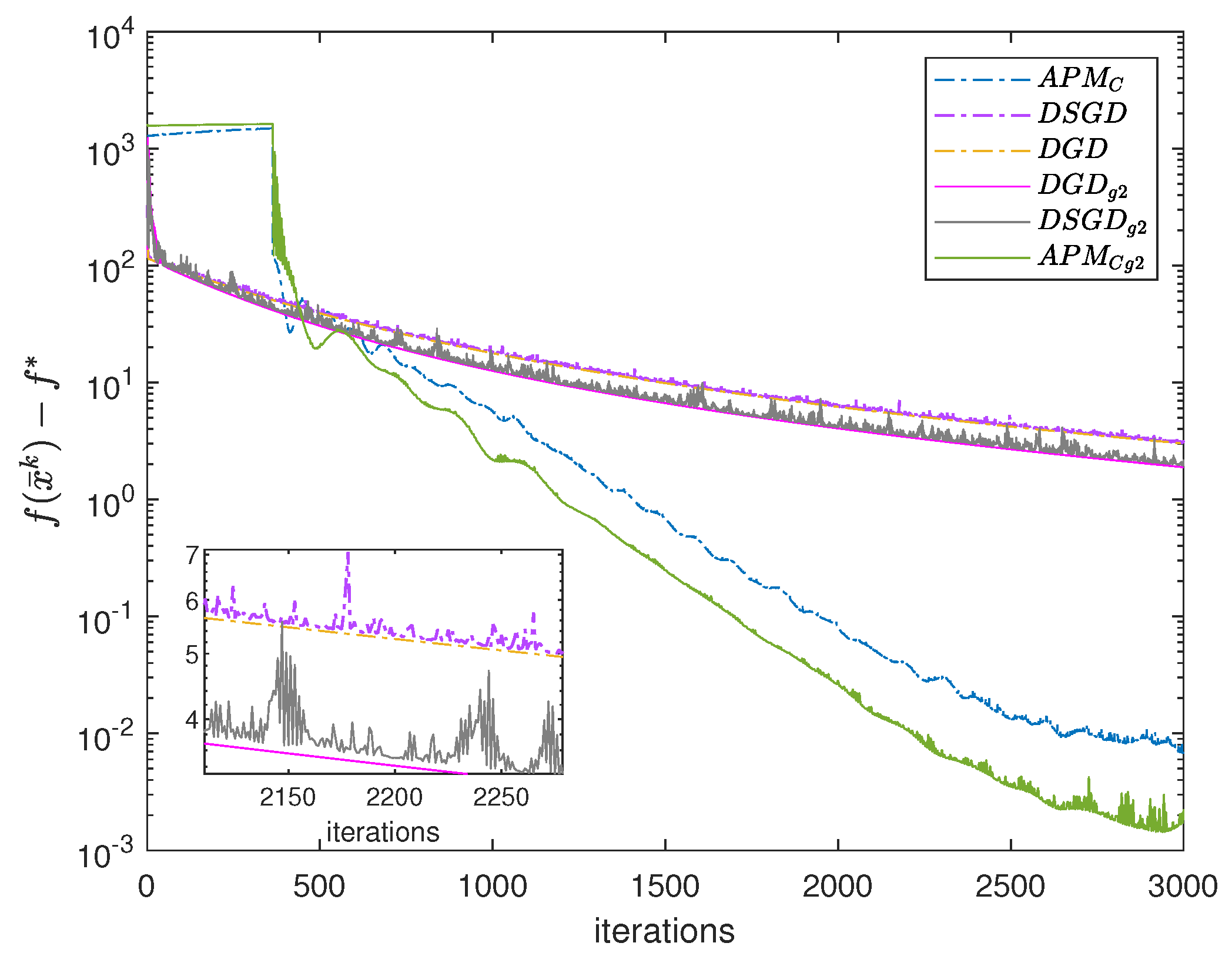
4.2. Decentralized Problem

We illustrate the performance of the decentralized extended gradient method ( D G D g 2 ) on the following problem
min x R p f ( x ) = i = 1 n f i ( x ) , with f i 1 2 M i x b i 2 + ν x 1 ,
where the random matrix M i R m × p is generated by the uniform distribution U ( 0 , 1 ) , and each column of M i is normalized to be 1. We set the parameters m = 512 , p = 1024 , r = 0.1 , ν = 0.0001 , and b i = M i x where x also follows the uniform distribution U ( 0 , 1 ) with sparsity r. The undirected graph is generated by Erdös-Rényi model [25] where each pair of nodes has the connection probability p = 0.8 , and the weight matrix W = I + M 2 , here M is generated with the Metropolis constant edge rules [26]. To demonstrate the effect of the previous gradient on the search direction of decentralized optimization algorithms, we use the sum of the gradients of the preceding two iterates ( g 2 ) to construct the search direction in the accelerated penalty method with consensus ( A P M C ) [27], the decentralized gradient descent (DGD) [21] and the decentralized stochastic gradient descent (DSGD) [28]. For DGD, DSGD, D G D g 2 and D S G D g 2 , we tune the optimized step size by hand, which are 0.09 , 0.9 , 0.058 and 0.58 , respectively. For A P M C and A P M C g 2 , the step sizes are 1 L and 0.1 1 L . The initial condition X 0 is 0 n × p . Compared to the original A P M C , DGD and DSGD, we can see from Figure 4 that the algorithms with the gradients of the preceding two iterates ( g 2 ) to construct search direction outperform than those with the current negative gradient as the search direction.
Finally, we extend the proposed method to a classification problem. First, we introduce the Radial Basis Function Network (RBFN) that uses a radial basis function ψ ( s ; c ) as the activation function, where s is a sample and c is a center. The output of the RBFN is a linear combination of radial basis functions ψ ( s ; c ) and the neuron weight parameters x. The training error that evaluates the performance of the RBFN can be written as (44). The training samples are { ( s 1 , 1 ) , , ( s N / 2 , 1 ) , ( s N / 2 + 1 , 1 ) , , ( s N , 1 ) } . The centers { c 1 , , c p } are randomly chosen from the training samples. The radial basis function is Gauss function ψ ( s , c ) = e s c 2 2 . The matrix M i represents ψ ( s i 1 ; c 1 ) ψ ( s i N / n ; c 1 ) ψ ( s i 1 ; c p ) ψ ( s i N / n ; c p ) , and b i R N / n is the corresponding sample label vector. We set N = 4000 , p = 300 and n = 20 . Each node holds samples set { s i m , b i m } m = 1 200 . For the decentralized extended gradient method, the step size is set as 1 L + μ . Figure 5 shows the classification result, and the accuracy of classing the samples is 1, which further indicates the efficiency of our method.

5. Conclusions

The gradient methods have been widely employed to solve the optimization problems. In this paper, we first introduce an extended gradient method for the centralized and decentralized smooth and strongly convex problems. Secondly, we establish the linear convergence of the extended gradient method in a centralized and decentralized manner, respectively. Finally, the numerical examples are used to demonstrate the convergence and to validate the efficiency compared to current classical methods. In the future, the acceleration technique used in this work can be applied to more optimization problems.

Author Contributions

Conceptualization, X.Z. and S.L.; methodology, X.Z.; software, X.Z. and N.Z.; validation, N.Z. and S.L.; investigation, X.Z.; Writing—Original draft preparation, X.Z.; Writing—Review and editing, S.L. and N.Z.; supervision, S.L. and N.Z.; funding acquisition, S.L. and N.Z. All authors have read and agreed to the published version of the manuscript.

Funding

This work was supported by the National Natural Science Foundation of China (Grant Nos. 12271419 and 12302033), and the Natural Science Basic Research Program of Shaanxi Province, China (Grant No. 2023-JC-QN-0009).

Data Availability Statement

No new data were created or analyzed in this study. Data sharing is not applicable to this article.

Conflicts of Interest

The authors declare that there are no conflict of interest with regards to the publication of this paper.

References

  1. Polyak, B.T. Some methods of speeding up the convergence of iteration methods. USSR Comput. Math. Math. Phys. 1964, 4, 1–17. [Google Scholar] [CrossRef]
  2. Ochs, P.; Brox, T.; Pock, T. iPiasco: Inertial Proximal Algorithm for Strongly Convex Optimization. J. Math. Imaging Vis. 2015, 53, 171–181. [Google Scholar] [CrossRef]
  3. Lessard, L.; Recht, B.; Packard, A. Analysis and design of optimization algorithms via integral quadratic constraints. SIAM J. Optim. 2016, 26, 57–95. [Google Scholar] [CrossRef]
  4. Hagedorn, M.; Jarre, F. Iteration Complexity of Fixed-Step-Momentum Methods for Convex Quadratic Functions. arXiv 2022, arXiv:2211.10234. [Google Scholar]
  5. Nesterov, Y. Introductory Lectures on Convex Optimization: A Basic Course; Springer: New York, NY, USA, 2003; Volume 87. [Google Scholar]
  6. Bertsekas, D. Convex Optimization Algorithms; Athena Scientific: Nashua, NH, USA, 2015. [Google Scholar]
  7. Popov, L.D. A modification of the Arrow-Hurwicz method for search of saddle points. Math. Notes Acad. Sci. USSR 1980, 28, 845–848. [Google Scholar] [CrossRef]
  8. Attouch, H.; Chbani, Z.; Fadili, J.; Riahi, H. First-order optimization algorithms via inertial systems with Hessian driven damping. Math. Program. 2022, 193, 113–155. [Google Scholar] [CrossRef]
  9. Ahmadi, M.J.; Arablouei, R.; Abdolee, R. Efficient estimation of graph signals with adaptive sampling. IEEE Trans. Signal Process. 2020, 68, 3808–3823. [Google Scholar] [CrossRef]
  10. Torkamani, R.; Zayyani, H.; Korki, M. Proportionate Adaptive Graph Signal Recovery. IEEE Trans. Signal Inf. Process. Netw. 2023, 9, 386–396. [Google Scholar] [CrossRef]
  11. Mai, V.; Johansson, M. Anderson acceleration of proximal gradient methods. International Conference on Machine Learning. PMLR 2020, 119, 6620–6629. [Google Scholar]
  12. Devolder, O.; Glineur, F.; Nesterov, Y. First-order methods of smooth convex optimization with inexact oracle. Math. Program. 2014, 146, 37–75. [Google Scholar] [CrossRef]
  13. Horn, R.A.; Johnson, C.R. Matrix Analysis; Cambridge University Press: Cambridge, UK, 2012. [Google Scholar]
  14. Poljak, B.T. Introduction to Optimization; Optimization Software, Inc.: New York, NY, USA, 1987. [Google Scholar]
  15. Khanh, P.D.; Mordukhovich, B.S.; Tran, D.B. Inexact reduced gradient methods in nonconvex optimization. J. Optim. Theory Appl. 2023. [Google Scholar] [CrossRef]
  16. Khanh, P.D.; Mordukhovich, B.S.; Tran, D.B. A New Inexact Gradient Descent Method with Applications to Nonsmooth Convex Optimization. arXiv 2023, arXiv:2303.08785. [Google Scholar]
  17. Schmidt, M.; Le Roux, N.; Bach, F. Minimizing finite sums with the stochastic average gradient. Math. Program. 2017, 162, 83–112. [Google Scholar] [CrossRef]
  18. Lee, J.D.; Lin, Q.; Ma, T.; Yang, T. Distributed stochastic variance reduced gradient methods by sampling extra data with replacement. J. Mach. Learn. Res. 2017, 18, 4404–4446. [Google Scholar]
  19. Jakovetić, D.; Xavier, J.; Moura, J.M.F. Fast distributed gradient methods. IEEE Trans. Autom. Control 2014, 59, 1131–1146. [Google Scholar] [CrossRef]
  20. Yuan, K.; Ling, Q.; Yin, W. On the convergence of decentralized gradient descent. SIAM J. Optim. 2016, 26, 1835–1854. [Google Scholar] [CrossRef]
  21. Nedic, A.; Ozdaglar, A. Distributed Subgradient Methods for Multi-Agent Optimization. IEEE Trans. Autom. Control 2009, 54, 48–61. [Google Scholar] [CrossRef]
  22. Berahas, A.S.; Bollapragada, R.; Keskar, N.S.; Wei, E. Balancing communication and computation in distributed optimization. IEEE Trans. Autom. Control 2018, 64, 3141–3155. [Google Scholar] [CrossRef]
  23. Shi, W.; Ling, Q.; Wu, G.; Yin, W. Extra: An exact first-order algorithm for decentralized consensus optimization. SIAM J. Optim. 2015, 25, 944–966. [Google Scholar] [CrossRef]
  24. Nedic, A.; Olshevsky, A.; Shi, W. Achieving geometric convergence for distributed optimization over time-varying graphs. SIAM J. Optim. 2017, 27, 2597–2633. [Google Scholar] [CrossRef]
  25. Erdös, P.; Rényi, A. On the evolution of random graphs. Publ. Math. Inst. Hung. Acad. Sci. 1960, 5, 17–60. [Google Scholar]
  26. Boyd, S.; Diaconis, P.; Xiao, L. Fastest mixing Markov chain on a graph. SIAM Rev. 2004, 46, 667–689. [Google Scholar] [CrossRef]
  27. Li, H.; Fang, C.; Yin, W.; Lin, Z. Decentralized Accelerated Gradient Methods With Increasing Penalty Parameters. IEEE Trans. Signal Process. 2020, 68, 4855–4870. [Google Scholar] [CrossRef]
  28. Chen, J.S.; Sayed, A.H. Diffusion Adaptation Strategies for Distributed Optimization and Learning Over Networks. IEEE Trans. Signal Process. 2012, 60, 4289–4305. [Google Scholar] [CrossRef]
Figure 1. Performance of optimization algorithms with three search directions.
Mathematics 11 04771 g001
Figure 2. Comparison of different algorithms for the least squares problem.
Mathematics 11 04771 g002
Figure 3. Performance of Nesterov accelerated gradient descent method and iPiasco with two search directions.
Mathematics 11 04771 g003
Figure 4. Comparison of different algorithms for the LASSO problem.
Mathematics 11 04771 g004
Figure 5. Classification result of the extended gradient method.
Mathematics 11 04771 g005
Disclaimer/Publisher’s Note: The statements, opinions and data contained in all publications are solely those of the individual author(s) and contributor(s) and not of MDPI and/or the editor(s). MDPI and/or the editor(s) disclaim responsibility for any injury to people or property resulting from any ideas, methods, instructions or products referred to in the content.

