Generalized Net Model of Heavy Oil Products’ Manufacturing in Petroleum Refinery

Abstract

Generalized nets (GNs) are a suitable tool for the modeling of parallel processes. Through them, it is possible to describe the functioning and results of the performance of complex real processes running in time. In a series of articles, we consistently describe the main processes involved in the production of petroleum products taking place in an oil refinery. The GN models can be used to track the actual processes in the oil refinery in order to monitor them, make decisions in case of changes in the environment, optimize some of the process components, and plan future actions. This study models the heavy oil production process in a refinery using the toolkit of GNs. Five processing units producing ten heavy-oil-refined products in an amount of 106.5 t/h from 443 t/h atmospheric residue feed, their blending, pipelines, and a tank farm devoted to storage of finished products consisting of three grades of fuel oil (very low sulfur fuel oil (0.5%S) —3.4 t/h; low sulfur fuel oil (1.0%S) —4.2 t/h; and high sulfur fuel oil (2.5%S) —66.9 t/h), and two grades of road pavement bitumen (bitumen 50/70 —30 t/h and bitumen 70/100 —2 t/h) are modeled in a GN medium. This study completes the process of modeling petroleum product production in an oil refinery using GNs. In this way, it becomes possible to construct a highly hierarchical model that incorporates the models already created for the production of individual petroleum products into a single entity, which allows for a comprehensive analysis of the refinery’s operations and decision making concerning the influence of various factors such as disruptions in the feedstock supply, the occurrence of unplanned shutdowns, optimization of the production process, etc.

1. Introduction

The processes that take place in an oil refinery where multiple products are produced from a single raw material (crude oil) are generally parallel and their description can be conveniently performed with the Generalized Net (GN, see [1]) toolbox. In the research we have carried out so far related to the modeling of the processes of production of automotive gasoline, diesel fuel for internal combustion engines, and gas products in a refinery, described in the articles [2,3,4], showed the possibility of modeling the production of these products using GNs. The part of the refinery scheme that produces heavy petroleum products has not yet been modeled using GNs.

The heavy oil is the residual oil fraction remaining after atmospheric distillation of the crude oil [5]. It contains components boiling above 360 °C and has specific gravity above 0.933 (API < 20) [6]. It is treated in the petroleum refinery to extract additional amounts of light oil products and produce heavy oil products like fuel oil, marine fuels, and road pavement bitumen [7,8,9,10,11]. All processes involved in the technological chain of heavy oil treatment have been the subject of modeling and simulation with the aim to better understand the behavior of the heavy oil plants and determine the values of the operation variables providing the optimum performance from economical, energy saving, and environmental points of view [12,13,14,15,16,17,18,19,20]. Gaikwad et al. [12] have simulated the operation of atmospheric residue vacuum distillation using Chemcad 5.1 software, with the aim to reduce the energy consumption. Mishra, and Yadav [13] have modeled an industrial slurry phase reactor (SPR) for vacuum residue hydrocracking using different kinetic models. Ye et al. [14] have employed a molecular-level reaction kinetic model of delayed coking of vacuum residue based on the structure-oriented lumping method to predict the product yield and group composition in the actual delayed coking process. Selalame et al. [15,16,17] have reviewed traditional modeling methodologies used in modeling and simulation of the fluid catalytic cracking (FCC) unit that converts vacuum gas oils and atmospheric residues into high-value light oil products. Wang et al. [18] have modeled and simulated a real-life industrial residue hydrotreating process based on Aspen HYSYS/Refining process simulation software. Sun et al. [19] have modeled and simulated the operation of a vapor recovery unit of an FCC complex using Aspen Plus process simulation software and reported a 2.4% reduction in medium pressure steam consumption. Piskunov et al. [20] have reviewed the main principles of modeling the dependencies of bitumen properties on their chemical composition, dispersed structure, and other quality parameters. All heavy oil models discussed in references [12,13,14,15,16,17,18,19,20] are partial models of diverse heavy oil treatment processes taking place in the petroleum refining. Their output is typically fed into linear programming refinery models to evaluate the most economically valuable scenario to follow during the oil-refining process [21,22]. In linear programming, the algorithm is performed step by step because it is sequential [23,24,25,26,27]. In contrast, the use of another approach to modeling processes which run in parallel as it is in the real world is the availing of Petri nets (see, e.g., [28]) and their extensions as Generalized Nets (GNs, see [1]).

Petri nets were employed for the short-term scheduling optimization of crude oil operations [29], while generalized nets (GN) were applied to model the processes of production of automotive gasoline [2], diesel fuels [3], and gas, LPG, propylene, and polypropylene [4] in a petroleum refinery.

The GN is a process description tool that can describe the processes in more details than Petri nets [4]. The complete analytics of any means of describing a real-world process (e.g., linear programming) can be described by the characteristics of the token characteristics in the GN model (see [4]), while the logic of the modeled process is represented by the predicates of the GN. For a more detailed discussion about the use of GN to model oil-refining processes, the reader can refer to our recent studies [2,3,4]. The method to the modeling of the processes of petroleum-refining product production by the use of generalized nets is original and all publications to date are the work of the authors.

Considering that the processes of production of automotive gasoline [2], diesel fuels [3], and gas, LPG, propylene, and polypropylene [4] in a petroleum refinery have been already modeled employing the toolkit of GN, the current research completes the modeling of all refined products by dealing with the process of production of different grades of heavy fuel oil and road pavement bitumen in the petroleum refinery, modeled by the use of generalized nets. Having modeled all processes of production of all oil-refining products in the petroleum refinery using distinct GNs enables the construction of a higher-level GN that encompasses the more detailed, already-established lower-level GN models. The higher-level GN model can be used to facilitate and optimize the decision-making process in the petroleum refining.

Our main goal is to describe the main processes in the oil refinery via a series of papers, based on which, using the hierarchical operators defined over the GNs (such operators do not exist for other types of Petri nets), we model the processes in the refinery as a whole. It is important to note that Petri net models are concerned with modeling individual pieces of the process, which does not allow for a single global model. This paper can also be seen as yet another application of the apparatus of GNs, which have, so far, been used to model various real-world processes in the fields of medicine, economics, education, industry, transportation, and others, with a major emphasis in computer science and artificial intelligence [30,31,32].

The aim of this research is to investigate the process of production of different grades of heavy fuel oil and road pavement bitumen in a petroleum refinery and model it by the use of GNs.

2. Materials and Methods

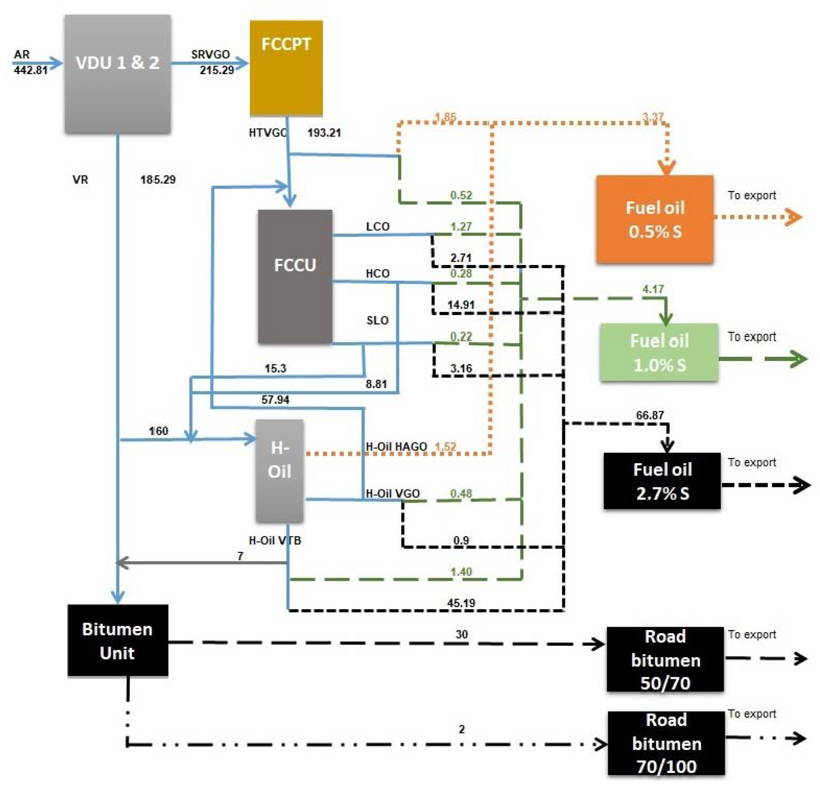
2.1. Processing Scheme for Production of Different Grades of Heavy Fuel Oil and Road Pavement Bitumen in a Petroleum Refinery to Be Modeled Using GNs

The fuel oils mainly used as fuels for cargo ships are also called marine fuels. The demand of marine fuels globally was reported to be 640,000 tons per day, highlighting the importance of this fuel for the world economics [33]. Three grades of fuel was produced in the refinery under study (LUKOIL Neftohim Burgas refinery): fuel oil having sulfur content ≤ 0.5 wt.% (Fuel oil 0.5% S); fuel oil having sulfur content ≤ 1.0 wt.% (Fuel oil 1.0% S); and fuel oil having sulfur content ≤ 2.5 wt.% (Fuel oil 2.5% S), as shown in Figure 1.

The specifications of the three fuel oil grades grades produced in the LUKOIL Neftohim Burgas (LNB) refinery are presented in

Table 1. Specification for fuel oil 0.5% S.

No	Properties	Unit	Min	Max	Test Method
			Value	Value
1	Density at 15 ${}^{°}$ C	kg/m${}^3$	-	991.0	BDS EN ISO 3675 [34]
					BDS EN ISO 12185 [35]
2	Kinematic viscosity at 50 ${}^{°}$C	mm${}^2$/s	-	380.0	BDS EN ISO 3104 [36]
					ASTM D 445 [37]
3	Calculated Carbon Aromaticity		-	870
	Index
4	Sulfur	% (m/m)	-	0.5	BDS EN ISO 8754 [38]
					ASTM D 4294 [39]
5	Flash point	${}^{°}$C	60	-	BDS EN ISO 2719 [40]
					ASTM D 93 (B) [41]
6	Hydrogen sulfide	mg/kg	-	2.00	IP 570 [42]
7	Acid number	mg KOH/g	-	2.5	ASTM D 664 [43]
8	Total sediment	% (m/m)	-	0.10	BDS ISO 10307-2 [44]
	Determination using standard				IP 390 [45]
	procedures for aging
	thermal aging (procedure A)
9	Carbon residue: micro method	% (m/m)	-	18.00	BDS EN ISO 10370 [46]
10	Pour point (upper)	${}^{°}$C	-	30	BDS EN ISO 3016 [47]
11	Water	% (V/V)	-	0.50	BDS EN ISO 3733 [48]
12	Ash	% (m/m)	-	0.100	BDS EN ISO 6245 [49]
13	Vanadium	mg/kg	-	350	IP 501, IP 470 [50,51]
14	Sodium	mg/kg	-	100	IP 501, IP 470 [52]
15	Aluminum + Silicon	mg/kg	-	60	IP 501, IP 470 [50,51]
					ISO 10478 [52]
16	Used lubricating oils (ULO):	mg/kg			IP 501, IP 470 [50,51]
	Calcium		>30
	and Zinc		>15
	or Calcium		>30
	and Phosphorus		>15

,

Table 2. Specification for Fuel oil 1.0% S.

No	Properties	Unit	Min	Max	Test Method
			Value	Value
1	Density at 15 ${}^{°}$C	kg/m${}^3$	-	995	BDS EN ISO 3675 [53]
					BDS EN ISO 12185 [34]
2	Kinematic viscosity at ${}^{°}$C	mm${}^2$/s	75	380	BDS EN ISO
					3104+AC ASTM [36]
					D 445 [37]
3	Sulfur content	% (m/m)	-	0.9	BDS EN ISO 8754 [38]
					ASTM D 4294 [39]
4	Water content	% (v/v)	-	1.0	BDS EN ISO 3733 [48]
5	Sediments, content	% (m/m)	-	0.5	BDS EN ISO 3735 [54]
6	Flash point in closed cup	${}^{°}$C	65	-	BDS EN ISO 2719 [40]
					ASTM D 93 (B) [41]
7	Pour point	${}^{°}$C	-	30	BDS EN ISO 3016 [47]
					ASTM D 97 [55]
8	Specific combustion heat (lower)	MJ/kg	40.2	-	ASTM D 240 [56]
					BDS ISO 8217 [57]
9	Carbon residue: micro method	% (m/m)	-	15	BDS EN ISO 10370 [46]
10	Ash content	% (m/m)	-	0.15	BDS EN ISO 6245 [49]
11	Total sediment
	Determination via hot filtration	% (m/m)	-	0.15	IP 375 [58]
					BDS ISO 10307-1 [59]
12	Nickel	mg/kg	-	60	IP 470, IP 501 [50,51]
13	Vanadium	mg/kg	-	120	IP 470, IP 501 [50,51]
14	Aluminum + Silicon	mg/kg	-	150	IP 470, IP 501 [50,51]
15	Sodium	mg/kg	-	40	IP 470, IP 501 [50,51]
16	Asphaltenes	% (m/m)	-	7	ASTM D 6560 [60]
					IP 143 [61]

and

Table 3. Specification for Fuel oil 2.5% S.

No	Properties	Unit	Min	Max	Test Method
			Value	Value
1	Density at 15 ${}^{°}$C	g/cm${}^3$	-	1.025	BDS EN ISO 3675 [34]
					ASTM D 1298 [62]
					BDS EN ISO 12185 [35]
2	Kinematic viscosity at 80 ${}^{°}$C	mm${}^2$/s	-	113.6	BDS EN ISO 3104 [36]
					ASTM D 445 [37]
	or Engler specific viscosity at	${}^{°}$E	-	15.0	BDS 1766-74 [63]
	80 ${}^{°}$C
3	Sulfur content	% (m/m)	-	2.5	BDS EN ISO 8754 [38]
					ASTM D 4294 [39]
4	Water content	% (m/m)	-	0.5 *	ASTM D 95 [64]
5	Mechanical impurities, content	% (m/m)	-	0.5 *	ASTM D 473 [65]
6	Flash point in open cup	${}^{°}$C	110	-	BDS EN ISO 2592 [66]
					ASTM D 92 [67]
7	Flash point in closed cup	${}^{°}$C	60	-	BDS EN ISO 2719 [40]
					ASTM D 93 (B) [41]
8	Pour point	${}^{°}$C	-	30	BDS EN ISO 3016 [47]
					ASTM D 97 [55]
9	Specific combustion heat	MJ/kg	39.8	-	ASTM D 4809 [53]
	(lower)				BDS ISO 8217 [57]
10	Ash content	% (m/m)	-	0.10	BDS EN ISO 6245 [49]
					ASTM D 482 [68]
11	Water soluble acids and alkaly		none	none	BDS 5252-84 [69]
12	Vanadium	ppm	-	300	ASTM D 5863 (A) [70]
					IP 470, IP 501 [50,51]
13	Polypropylene		free	free	BP/V.4/09-99
14	Conradson Carbon residue	% (m/m)	-	18	ASTM D 189 [71]
					ASTM D 4530 [72]
15	Asphaltenes	% (m/m)	to be	repor	ASTM D 6560 [60]
				ted	IP 143 [61]

* The total value of p. (4 + 5) does not exceed 0.5% (m/m).

. The fuel oil products manufactured in the LNB refinery are marketed on the basis of the specifications shown in Table 1, Table 2 and Table 3.

The components for production of these three grades of fuel oils are hydrotreated vacuum gas oil (HTVGO); fluid catalytic cracking (FCC) light cycle oil (LCO); FCC heavy cycle oil (HCO); FCC slurry oil (SLO); H-Oil heavy atmospheric gas oil (H-Oil HAGO); H-Oil vacuum gas oil (H-Oil VGO); and an H-Oil hydrocracked vacuum residue called vacuum tower bottom (H-Oil VTB). Their physicochemical properties are summarized in

Table 4. Physicochemical properties of heavy oils participating in the processing scheme of heavy oil products manufactured in the LUKOIL Neftohim Burgas refinery under study.

Properties	AR	SRVGO	SRVR	HTVGO	FCC LCO	FCC HCO	FCC SLO	H-Oil HAGO	H-Oil VGO	H-Oil VTB
Density at 15 ${}^{°}$C, g/cm${}^3$	0.9408	0.9200	1.0024	0.9030	0.9412	1.0336	1.1146	0.9504	0.9707	1.025
HTSD (ASTM D-7169)
IBP	310	321	433	348	138	196	196	313	320	432
5	371	361	496	365	177	251	321	342	347	494
10	398	378	520	377	195	267	341	355	361	522
20	434	402	551	387	207	281	366	364	371	573
30	466	420	575	396	220	296	383	372	380	591
40	498	435	596	403	230	306	399	379	389	591
50	531	451	617	411	232	321	413	386	397	609
60	567	466	638	418	247	332	428	393	404	629
70	604	483	657	426	253	344	444	398	411	651
80	642	501	681	433	258	358	463	404	419	679
90	684	525	708	439	272	379	487	410	428	712
95	705	544	722	445	282	397	506	417	435
FBP				453	319	446	539	424	442
Sulfur, wt.%	2.34	1.78	2.84	0.20	0.20	0.80	0.95	0.753	0.85	1.12
Viscosity at 80 ${}^{°}$C,	72.0	14.8	3000	12.6	1.35	2.91	56.7	12.9	16.7	2172
mm${}^2$/s
Softening point, ${}^{°}$C			40.0							36.0
Saturates, wt.%	50.0	55.3	25.6	60.3	19.9	18.2	15.1	48.8	40.6	26.0
Aromatics, wt.%	36.8	42.8	52.5	39.3	80.1	76.4	53.8	49.0	56.9	50.9
Resins, wt.%	6.5	1.9	7.8	0.4	0	5.4	27.6	2.2	2.5	7.0
Asphaltenes, wt.%	6.7	0	14.1	0	0	0	3.5	0	0	16.1

. These components are produced in the petroleum-refining units: a fluid catalytic cracking feed hydrotreater or a pretreater (FCCPT); fluid catalytic cracking (FCCU); and H-Oil ebullated bed vacuum residue hydrocracking (H-Oil). Details about the performance of these refining units and the qualities of their products are given in our earlier research [73].

Figure 1 indicates that the production of road pavement bitumen takes place in the bitumen unit where a blend of straight run vacuum residue and H-Oil VTB are oxidized to manufacture two grades of bitumen: Road bitumen 50/70 and Road bitumen 70/100. The specifications of the two road bitumen grades are presented in

Table 5. Specification for road bitumen grade 50/70.

No	Properties	Unit	Min	Max	Test Method
			Value	Value
1	Penetration at 25 ${}^{°}$C	0.1mm	50	70	BDS EN 1426 [37]
2	Softening point	${}^{°}$C	46.0	54.0	BDS EN 1427 [74]
3	Fraass breaking point	${}^{°}$C	-	minus 8	BDS EN 12593 [75]
4	Flash point	${}^{°}$C	230	-	BDS EN ISO 2592 [76]
5	Resistance to hardening, ${}^{°}$C				EN 12607-1 [66]
	at 163
	• change in mass (absolute value)	% (m/m)	-	0.5
	• retained penetration	% (m/m)	50	-	BDS EN 1426 [77]
	• increase in softening point	${}^{°}$C	-	9	BDS EN 1427 [78]
6	Solubility	% (m/m)	99.0	-	BDS EN 12592 [79]
7	Paraffin wax content	% (m/m)	-	2.2	BDS EN 12606-1 [54]

and

Table 6. Specification for road bitumen grade 70/100.

No	Properties	Unit	Min	Max	Test Method
			Value	Value
1	Penetration at 25 ${}^{°}$C	0.1mm	70	100	BDS EN 1426 [37]
2	Softening point	${}^{°}$C	43.0	51.0	BDS EN 1427 [74]
3	Fraass breaking point	${}^{°}$C	-	minus 10	BDS EN 12593 [75]
4	Flash point	${}^{°}$C	230	-	BDS EN ISO 2592 [76]
5	Resistance to hardening, ${}^{°}$C				EN 12607-1 [66]
	at 163
	• change in mass (absolute value)	% (m/m)	-	0.8
	• retained penetration	% (m/m)	46	-	BDS EN 1426 [77]
	• increase in softening point	${}^{°}$C	-	9	BDS EN 1427 [78]
6	Solubility	% (m/m)	99.0	-	BDS EN 12592 [79]
7	Paraffin wax content	% (m/m)	-	2,2	BDS EN 12606-17 [54]

.

Details about the production of road pavement bitumen from straight run vacuum residue (VR) and H-Oil VTB can be found in our recent research [73]. Figure 1 also shows that the Vacuum Residue (VR) and the vacuum gas oil (SRVGO) availed to produce the components for the manufacture of the fuel oil grades, and so the road pavement bitumen are obtained in the vacuum distillation units (VDU 1 and 2), where the atmospheric residue derived from the crude distillation units is fractionated. Details about the performance of the vacuum distillation units are explained in [12].

2.2. Short Notes on the Theory of GNs

A full description of the GNs is given in [1]; short one, e.g., in [4]. So, here we will mention only that the GNs, in contrast to Petri nets, have tokens that enter the net with initial characteristics, and at the time of their transfer in the net, they obtain their next characteristics, having the possibility to collect all received characteristics if this is necessary for the concrete model.

The second important difference between Petri nets and GNs is in the existence of predicates associated with the separate GN transitions that determine the directions of the token’s transfers. Both of these ideas in their full form were introduced for the first time for GNs. On one hand, they are extensions of the colored Petri nets [80], because each token’s color can be represent as a token’s characteristic, and on the other hand, the special matrices of the transition condition predicates are essential extensions of the idea for the predicate transition nets (see [81]). The concept of an Index Matrix (IM, see, e.g., [82]) was introduced in 1987, especially for the needs of a mathematical description of the operations with GN transitions (see [1]).

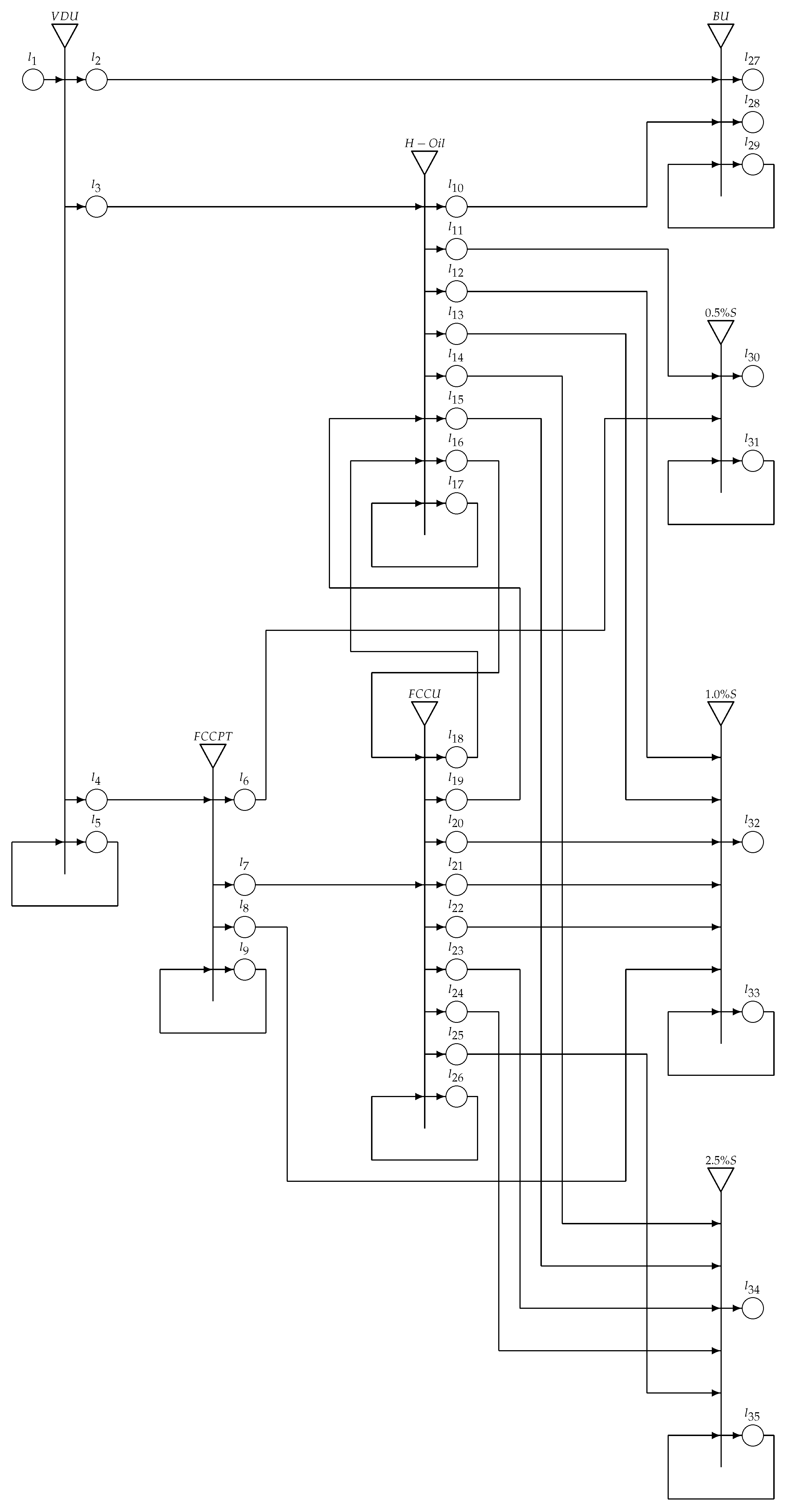
3. Results of Modeling Heavy Oil Product Manufacturing in a Petroleum Refinery Using Generalized Nets

The GN model contains 8 transitions, 35 places, and 8 types of tokens (see Figure 2).

The meaning of the transitions is as follows:

•

VDU—Vacuum distillation unit

•

FCCPT—Fluid catalytic cracking feed pretreater

•

H-Oil—H-Oil vacuum residue hydrocracker

•

FCCU—Fluid catalytic cracking unit

•

BU—Road pavement (asphalt) bitumen production unit

•

0.5 S—Fuel oil containing maximum of 0.5 wt.% sulfur

•

1.0 S—Fuel oil containing maximum of 1.0 wt.% sulfur

•

2.5 S—Fuel oil containing maximum of 2.5 wt.% sulfur

In the initial time moment of the GN functioning, token ${\alpha }_0$ stays in place $l_1$ with an initial characteristic

$$“\mathrm{A}\mathrm{t}\mathrm{m}\mathrm{o}\mathrm{s}\mathrm{p}\mathrm{h}\mathrm{e}\mathrm{r}\mathrm{i}\mathrm{c} \mathrm{R}\mathrm{e}\mathrm{s}\mathrm{i}\mathrm{d}\mathrm{u}\mathrm{e} \left(\mathrm{A}\mathrm{R}\right), \mathrm{i}\mathrm{n}\mathrm{i}\mathrm{t}\mathrm{i}\mathrm{a}\mathrm{l} \mathrm{q}\mathrm{u}\mathrm{a}\mathrm{n}\mathrm{t}\mathrm{i}\mathrm{t}\mathrm{y}”;$$

token ${\beta }_0$ stays in place $l_9$ with an initial characteristic

$$“\mathrm{S}\mathrm{t}\mathrm{r}\mathrm{a}\mathrm{i}\mathrm{g}\mathrm{h}\mathrm{t} \mathrm{r}\mathrm{u}\mathrm{n} \mathrm{v}\mathrm{a}\mathrm{c}\mathrm{u}\mathrm{u}\mathrm{m} \mathrm{g}\mathrm{a}\mathrm{s} \mathrm{o}\mathrm{i}\mathrm{l} \left(\mathrm{S}\mathrm{R}\mathrm{V}\mathrm{G}\mathrm{O}\right), \mathrm{i}\mathrm{n}\mathrm{i}\mathrm{t}\mathrm{i}\mathrm{a}\mathrm{l} \mathrm{q}\mathrm{u}\mathrm{a}\mathrm{n}\mathrm{t}\mathrm{i}\mathrm{t}\mathrm{y}”;$$

token ${\gamma }_0$ stays in place $l_{17}$ with an initial characteristic

$$“\mathrm{B}\mathrm{l}\mathrm{e}\mathrm{n}\mathrm{d} \mathrm{o}\mathrm{f} \mathrm{s}\mathrm{t}\mathrm{r}\mathrm{a}\mathrm{i}\mathrm{g}\mathrm{h}\mathrm{t} \mathrm{r}\mathrm{u}\mathrm{n} \mathrm{v}\mathrm{a}\mathrm{c}\mathrm{u}\mathrm{u}\mathrm{m} \mathrm{r}\mathrm{e}\mathrm{s}\mathrm{i}\mathrm{d}\mathrm{u}\mathrm{e} \left(\mathrm{S}\mathrm{R}\mathrm{V}\mathrm{R}\right), \mathrm{F}\mathrm{C}\mathrm{C} \mathrm{H}\mathrm{C}\mathrm{O}, \mathrm{a}\mathrm{n}\mathrm{d} \mathrm{F}\mathrm{C}\mathrm{C} \mathrm{S}\mathrm{L}\mathrm{O}, \mathrm{i}\mathrm{n}\mathrm{i}\mathrm{t}\mathrm{i}\mathrm{a}\mathrm{l} \mathrm{q}\mathrm{u}\mathrm{a}\mathrm{n}\mathrm{t}\mathrm{i}\mathrm{t}\mathrm{y}”;$$

token ${\delta }_0$ stays in place $l_{26}$ with an initial characteristic

$$“\mathrm{B}\mathrm{l}\mathrm{e}\mathrm{n}\mathrm{d} \mathrm{o}\mathrm{f} \mathrm{v}\mathrm{a}\mathrm{c}\mathrm{u}\mathrm{u}\mathrm{m} \mathrm{g}\mathrm{a}\mathrm{s} \mathrm{o}\mathrm{i}\mathrm{l}\mathrm{s} \mathrm{c}\mathrm{o}\mathrm{n}\mathrm{s}\mathrm{i}\mathrm{s}\mathrm{t}\mathrm{i}\mathrm{n}\mathrm{g} \mathrm{o}\mathrm{f} \mathrm{S}\mathrm{R}\mathrm{V}\mathrm{G}\mathrm{O}, \mathrm{a}\mathrm{n}\mathrm{d} \mathrm{H}-\mathrm{O}\mathrm{i}\mathrm{l} \mathrm{V}\mathrm{G}\mathrm{O}, \mathrm{i}\mathrm{n}\mathrm{i}\mathrm{t}\mathrm{i}\mathrm{a}\mathrm{l} \mathrm{q}\mathrm{u}\mathrm{a}\mathrm{n}\mathrm{t}\mathrm{i}\mathrm{t}\mathrm{y}”;$$

token ${ϵ}^{}0$ stays in place $l_{29}$ with an initial characteristic

$$“\mathrm{B}\mathrm{l}\mathrm{e}\mathrm{n}\mathrm{d} \mathrm{o}\mathrm{f} \mathrm{S}\mathrm{R}\mathrm{V}\mathrm{R}, \mathrm{a}\mathrm{n}\mathrm{d} \mathrm{h}\mathrm{y}\mathrm{d}\mathrm{r}\mathrm{o}\mathrm{c}\mathrm{r}\mathrm{a}\mathrm{c}\mathrm{k}\mathrm{e}\mathrm{d} \mathrm{v}\mathrm{a}\mathrm{c}\mathrm{u}\mathrm{u}\mathrm{m} \mathrm{r}\mathrm{e}\mathrm{s}\mathrm{i}\mathrm{d}\mathrm{u}\mathrm{e}, \mathrm{i}\mathrm{n}\mathrm{i}\mathrm{t}\mathrm{i}\mathrm{a}\mathrm{l} \mathrm{q}\mathrm{u}\mathrm{a}\mathrm{n}\mathrm{t}\mathrm{i}\mathrm{t}\mathrm{y}”;$$

token ${\zeta }_0$ stays in place $l_{31}$ with an initial characteristic

$$“\mathrm{F}\mathrm{u}\mathrm{e}\mathrm{l} \mathrm{o}\mathrm{i}\mathrm{l} \mathrm{w}\mathrm{i}\mathrm{t}\mathrm{h} \mathrm{m}\mathrm{a}\mathrm{x}\mathrm{i}\mathrm{m}\mathrm{u}\mathrm{m} \mathrm{s}\mathrm{u}\mathrm{l}\mathrm{f}\mathrm{u}\mathrm{r} \mathrm{c}\mathrm{o}\mathrm{n}\mathrm{t}\mathrm{e}\mathrm{n}\mathrm{t} \mathrm{o}\mathrm{f} 0.5 \mathrm{w}\mathrm{t}.\%, \mathrm{i}\mathrm{n}\mathrm{i}\mathrm{t}\mathrm{i}\mathrm{a}\mathrm{l} \mathrm{q}\mathrm{u}\mathrm{a}\mathrm{n}\mathrm{t}\mathrm{i}\mathrm{t}\mathrm{y}”;$$

token ${\eta }_0$ stays in place $l_{33}$ with an initial characteristic

$$“\mathrm{F}\mathrm{u}\mathrm{e}\mathrm{l} \mathrm{o}\mathrm{i}\mathrm{l} \mathrm{w}\mathrm{i}\mathrm{t}\mathrm{h} \mathrm{m}\mathrm{a}\mathrm{x}\mathrm{i}\mathrm{m}\mathrm{u}\mathrm{m} \mathrm{s}\mathrm{u}\mathrm{l}\mathrm{f}\mathrm{u}\mathrm{r} \mathrm{c}\mathrm{o}\mathrm{n}\mathrm{t}\mathrm{e}\mathrm{n}\mathrm{t} \mathrm{o}\mathrm{f} 1.0 \mathrm{w}\mathrm{t}.\%, \mathrm{i}\mathrm{n}\mathrm{i}\mathrm{t}\mathrm{i}\mathrm{a}\mathrm{l} \mathrm{q}\mathrm{u}\mathrm{a}\mathrm{n}\mathrm{t}\mathrm{i}\mathrm{t}\mathrm{y}”;$$

token ${\theta }_0$ stays in place $l_{35}$ with an initial characteristic

$$“\mathrm{F}\mathrm{u}\mathrm{e}\mathrm{l} \mathrm{o}\mathrm{i}\mathrm{l} \mathrm{w}\mathrm{i}\mathrm{t}\mathrm{h} \mathrm{m}\mathrm{a}\mathrm{x}\mathrm{i}\mathrm{m}\mathrm{u}\mathrm{m} \mathrm{s}\mathrm{u}\mathrm{l}\mathrm{f}\mathrm{u}\mathrm{r} \mathrm{c}\mathrm{o}\mathrm{n}\mathrm{t}\mathrm{e}\mathrm{n}\mathrm{t} \mathrm{o}\mathrm{f} 2.5 \mathrm{w}\mathrm{t}.\%, \mathrm{i}\mathrm{n}\mathrm{i}\mathrm{t}\mathrm{i}\mathrm{a}\mathrm{l} \mathrm{q}\mathrm{u}\mathrm{a}\mathrm{n}\mathrm{t}\mathrm{i}\mathrm{t}\mathrm{y}”;$$

In each next time-moment, tokens ${\alpha }_1,{\alpha }_2,...$ enter place $l_1$ with initial characteristics

$$“\mathrm{A}\mathrm{R}, \mathrm{c}\mathrm{u}\mathrm{r}\mathrm{r}\mathrm{e}\mathrm{n}\mathrm{t} \mathrm{a}\mathrm{r}\mathrm{r}\mathrm{i}\mathrm{v}\mathrm{i}\mathrm{n}\mathrm{g} \mathrm{q}\mathrm{u}\mathrm{a}\mathrm{n}\mathrm{t}\mathrm{i}\mathrm{t}\mathrm{y}”.$$

For brevity, below, we will denote these tokens as $\alpha$ without their (current) lower indices. Following the same way, we will omit the lower indices of the $\beta$-$\gamma$ and $\delta$-tokens, the sense of which will be described below.

The GN transitions have the following forms.

$$VDU=〈\{l_1,l_5\},\{l_2,l_3,l_4,l_5\},\begin{array}{ccccc}& l_2& l_3& l_4& l_4\\ l_1& false& false& false& true\\ l_5& W_{5,2}& W_{5,3}& W_{5,4}& true\end{array}〉,$$

where

• $W_{5,2}=$“there is a request for AR from BU”,
• $W_{5,3}=$“there is a request for AR from H-Oil”,
• $W_{5,4}=$“there is a request for AR from FCCPT”.

When $\alpha$-token enters place $l_1$, on the next time moment, it enters place $l_5$ and unites with token ${\alpha }_0$ that obtains the characteristic

$$“\mathrm{A}\mathrm{R}, \mathrm{c}\mathrm{u}\mathrm{r}\mathrm{r}\mathrm{e}\mathrm{n}\mathrm{t} \mathrm{q}\mathrm{u}\mathrm{a}\mathrm{n}\mathrm{t}\mathrm{i}\mathrm{t}\mathrm{y} \mathrm{i}\mathrm{n} \mathrm{t}\mathrm{h}\mathrm{e} \mathrm{r}\mathrm{e}\mathrm{s}\mathrm{e}\mathrm{r}\mathrm{v}\mathrm{o}\mathrm{i}\mathrm{r}”.$$

With respect to the truth values of predicates $W_{5,2},W_{5,3},W_{5,4}$, token ${\alpha }_0$ splits into two, three, or four tokens–the same token ${\alpha }_0$ continues to stay in place $l_5$ with the above-mentioned characteristic, and tokens ${\alpha }^1,{\alpha }^2$ and/or ${\alpha }^3$, obtain, respectively, the characteristics

$$“q_1 \mathrm{A}\mathrm{R} \mathrm{f}\mathrm{o}\mathrm{r} \mathrm{B}\mathrm{U}”$$

in place $l_2$, where $q_1\in [0,Q_1]$;

$$“q_2 \mathrm{A}\mathrm{R} \mathrm{f}\mathrm{o}\mathrm{r} \mathrm{H}-\mathrm{O}\mathrm{i}\mathrm{l}”$$

in place $l_3$, where $q_2\in [0,Q_2]$;

$$“q_3 \mathrm{A}\mathrm{R} \mathrm{f}\mathrm{o}\mathrm{r} \mathrm{F}\mathrm{C}\mathrm{C}\mathrm{P}\mathrm{T}”$$

in place $l_4$, where $q_3\in [0,Q_3]$.

Here and below, $Q_i$ is the maximal quantity for the i-th heavy oil component participating in the production of fuel oil and road pavement bitumen, where $1\le i\le 26$.

$$FUCPT=〈\{l_4,l_9\},\{l_6,l_7,l_8,l_9\},\begin{array}{ccccc}& l_6& l_7& l_8& l_8\\ l_1& false& false& false& true\\ l_9& W_{9,6}& W_{9,7}& W_{9,8}& true\end{array}〉,$$

where

• $W_{9,6}$ = “there is a request for HTVGO for production of fuel oil with maximum sulfur content of 0.5% S”,
• $W_{9,7}$ = “there is a request for HTVGO as a feed for fluid catalytic cracking unit”,
• $W_{9,8}$ = “there is a request for HTVGO for production of fuel oil with maximum sulfur content of 1.0% S”.

The ${\alpha }^3$-token from place $l_4$ enters place $l_9$ and unites with token ${\beta }_0$ that obtains the characteristic

$$“\mathrm{B}\mathrm{l}\mathrm{e}\mathrm{n}\mathrm{d} \mathrm{o}\mathrm{f} \mathrm{v}\mathrm{a}\mathrm{c}\mathrm{u}\mathrm{u}\mathrm{m} \mathrm{g}\mathrm{a}\mathrm{s} \mathrm{o}\mathrm{i}\mathrm{l}\mathrm{s} \mathrm{c}\mathrm{o}\mathrm{n}\mathrm{s}\mathrm{i}\mathrm{s}\mathrm{t}\mathrm{i}\mathrm{n}\mathrm{g} \mathrm{o}\mathrm{f} \mathrm{S}\mathrm{R}\mathrm{V}\mathrm{G}\mathrm{O}, \mathrm{a}\mathrm{n}\mathrm{d} \mathrm{H}-\mathrm{O}\mathrm{i}\mathrm{l} \mathrm{V}\mathrm{G}\mathrm{O}, \mathrm{c}\mathrm{u}\mathrm{r}\mathrm{r}\mathrm{e}\mathrm{n}\mathrm{t} \mathrm{q}\mathrm{u}\mathrm{a}\mathrm{n}\mathrm{t}\mathrm{i}\mathrm{t}\mathrm{y}$$

$$\mathrm{i}\mathrm{n} \mathrm{t}\mathrm{h}\mathrm{e} \mathrm{r}\mathrm{e}\mathrm{s}\mathrm{e}\mathrm{r}\mathrm{v}\mathrm{o}\mathrm{i}\mathrm{r}”.$$

With respect to the truth values of predicates $W_{9,6},W_{9,7},W_{9,8}$, token ${\beta }_0$ splits into two, three, or four tokens–the same token ${\beta }_0$ continues to stay in place $l_9$ with the above-mentioned characteristic, and tokens ${\beta }^1,{\beta }^2$ and/or ${\beta }^3$, obtain, respectively, the characteristics

$$“q_4 \mathrm{H}\mathrm{T}\mathrm{V}\mathrm{G}\mathrm{O} \mathrm{f}\mathrm{o}\mathrm{r} \mathrm{f}\mathrm{u}\mathrm{e}\mathrm{l} \mathrm{o}\mathrm{i}\mathrm{l} \mathrm{w}\mathrm{i}\mathrm{t}\mathrm{h} \mathrm{m}\mathrm{a}\mathrm{x}\mathrm{i}\mathrm{m}\mathrm{u}\mathrm{m} \mathrm{s}\mathrm{u}\mathrm{l}\mathrm{f}\mathrm{u}\mathrm{r} \mathrm{c}\mathrm{o}\mathrm{n}\mathrm{t}\mathrm{e}\mathrm{n}\mathrm{t} \mathrm{o}\mathrm{f} 0.5\% \mathrm{f}\mathrm{o}\mathrm{r} \mathrm{F}\mathrm{C}\mathrm{C}\mathrm{U}”$$

in place $l_6$, where $q_4\in [0,Q_4]$;

$$“q_5 \mathrm{H}\mathrm{T}\mathrm{V}\mathrm{G}\mathrm{O} \mathrm{f}\mathrm{o}\mathrm{r} \mathrm{f}\mathrm{l}\mathrm{u}\mathrm{i}\mathrm{d} \mathrm{c}\mathrm{a}\mathrm{t}\mathrm{a}\mathrm{l}\mathrm{y}\mathrm{t}\mathrm{i}\mathrm{c} \mathrm{c}\mathrm{r}\mathrm{a}\mathrm{c}\mathrm{k}\mathrm{i}\mathrm{n}\mathrm{g} \mathrm{u}\mathrm{n}\mathrm{i}\mathrm{t}”$$

in place $l_7$, where $q_5\in [0,Q_5]$;

$$“q_6 \mathrm{H}\mathrm{T}\mathrm{V}\mathrm{G}\mathrm{O} \mathrm{f}\mathrm{o}\mathrm{r} \mathrm{F}\mathrm{u}\mathrm{e}\mathrm{l} \mathrm{o}\mathrm{i}\mathrm{l} \mathrm{w}\mathrm{i}\mathrm{t}\mathrm{h} \mathrm{m}\mathrm{a}\mathrm{x}\mathrm{i}\mathrm{m}\mathrm{u}\mathrm{m} \mathrm{s}\mathrm{u}\mathrm{l}\mathrm{f}\mathrm{u}\mathrm{r} \mathrm{c}\mathrm{o}\mathrm{n}\mathrm{t}\mathrm{e}\mathrm{n}\mathrm{t} \mathrm{o}\mathrm{f} 1.0 \mathrm{w}\mathrm{t}.\% \mathrm{S}”$$

in place $l_8$, where $q_6\in [0,Q_6]$.

$$H-Oil=〈\{l_3,l_{17},l_{18},l_{19}\},\{l_{10},l_{11},l_{12},l_{13},l_{14},l_{15},l_{16},l_{17}\},$$

$$\begin{array}{ccccccccc}& l_{10}& l_{11}& l_{12}& l_{13}& l_{14}& l_{15}& l_{16}& l_{16}\\ l_1& false& false& false& false& false& false& false& true\\ l_{17}& W_{17,10}& W_{17,11}& W_{17,12}& W_{17,13}& W_{17,14}& W_{17,15}& W_{17,16}& true\\ l_{18}& false& false& false& false& false& false& false& true\\ l_{19}& false& false& false& false& false& false& false& true\end{array}〉,$$

where

$W_{17,10}$ = “there is a request for VTB for Bitumen”,

$W_{17,11}$ = “there is a request for HAGO for Fuel oil 0.5% S”,

$W_{17,12}$ = “there is a request for VGO for Fuel oil 1.0% S”,

$W_{17,13}$ = “there is a request for VTB for Fuel oil 1.0% S”,

$W_{17,14}$ = “there is a request for VTB for Fuel oil 2.5% S”,

$W_{17,15}$ = “there is a request for VGO for Fuel oil 2.5% S”,

$W_{17,16}$ = “there is a request for VGO as a feed for FCCU”.

The ${\alpha }^2$-token from place $l_3$ enters place $l_{17}$ and unites with token ${\gamma }_0$ that obtains the characteristic

$$“\mathrm{S}\mathrm{t}\mathrm{r}\mathrm{a}\mathrm{i}\mathrm{g}\mathrm{h}\mathrm{t} \mathrm{r}\mathrm{u}\mathrm{n} \mathrm{v}\mathrm{a}\mathrm{c}\mathrm{u}\mathrm{u}\mathrm{m} \mathrm{r}\mathrm{e}\mathrm{s}\mathrm{i}\mathrm{d}\mathrm{u}\mathrm{e} \left(\mathrm{S}\mathrm{R}\mathrm{V}\mathrm{R}\right), \mathrm{c}\mathrm{u}\mathrm{r}\mathrm{r}\mathrm{e}\mathrm{n}\mathrm{t} \mathrm{q}\mathrm{u}\mathrm{a}\mathrm{n}\mathrm{t}\mathrm{i}\mathrm{t}\mathrm{y} \mathrm{i}\mathrm{n} \mathrm{t}\mathrm{h}\mathrm{e} \mathrm{r}\mathrm{e}\mathrm{s}\mathrm{e}\mathrm{r}\mathrm{v}\mathrm{o}\mathrm{i}\mathrm{r}”.$$

With respect to the truth values of predicates $W_{17,10},...,W_{17,16}$, token ${\gamma }_0$ splits into two, three, ..., or seven tokens—the same token ${\gamma }_0$ continues to stay in place $l_{17}$ with the above-mentioned characteristic, and tokens ${\gamma }^1,...$ and/or ${\gamma }^7$, obtain, respectively, the characteristics

$$“q_7 VTB for BU”$$

in place $l_{10}$, where $q_7\in [0,Q_7]$;

$$“q_8 \mathrm{H}\mathrm{A}\mathrm{G}\mathrm{O} \mathrm{f}\mathrm{o}\mathrm{r} \mathrm{F}\mathrm{u}\mathrm{e}\mathrm{l} \mathrm{o}\mathrm{i}\mathrm{l} 0.5\% \mathrm{S}”$$

in place $l_{11}$, where $q_8\in [0,Q_8]$;

$$“q_9 \mathrm{V}\mathrm{G}\mathrm{O} \mathrm{f}\mathrm{o}\mathrm{r} \mathrm{F}\mathrm{u}\mathrm{e}\mathrm{l} \mathrm{o}\mathrm{i}\mathrm{l} 1.0\% \mathrm{S}”$$

in place $l_{12}$, where $q_9\in [0,Q_9]$;

$$“q_{10} \mathrm{V}\mathrm{T}\mathrm{B} \mathrm{f}\mathrm{o}\mathrm{r} \mathrm{F}\mathrm{u}\mathrm{e}\mathrm{l} \mathrm{o}\mathrm{i}\mathrm{l} 1.0\% \mathrm{S}”$$

in place $l_{13}$, where $q_{10}\in [0,Q_{10}]$;

$$“q_{11} \mathrm{V}\mathrm{T}\mathrm{B} \mathrm{f}\mathrm{o}\mathrm{r} \mathrm{F}\mathrm{u}\mathrm{e}\mathrm{l} \mathrm{o}\mathrm{i}\mathrm{l} 2.5\% \mathrm{S}”$$

in place $l_{14}$, where $q_{11}\in [0,Q_{11}]$;

$$“q_{12} \mathrm{V}\mathrm{G}\mathrm{O} \mathrm{f}\mathrm{o}\mathrm{r} \mathrm{F}\mathrm{u}\mathrm{e}\mathrm{l} \mathrm{o}\mathrm{i}\mathrm{l} 2.5\% \mathrm{S}”$$

in place $l_{15}$, where $q_{12}\in [0,Q_{12}]$;

$$“q_{13} \mathrm{V}\mathrm{G}\mathrm{O} \mathrm{a}\mathrm{s} \mathrm{a} \mathrm{f}\mathrm{e}\mathrm{e}\mathrm{d} \mathrm{f}\mathrm{o}\mathrm{r} \mathrm{F}\mathrm{C}\mathrm{C}\mathrm{U} \mathrm{f}\mathrm{o}\mathrm{r} \mathrm{F}\mathrm{C}\mathrm{C}\mathrm{U}”$$

in place $l_{16}$, where $q_{13}\in [0,Q_{13}]$.

$$FCCU=〈\{l_7,l_{16},l_{26},\},\{l_{18},l_{19},l_{20},l_{21},l_{22},l_{23},l_{24},l_{25},l_{26}\},$$

$$\begin{array}{cccccccccc}& l_{18}& l_{19}& l_{20}& l_{21}& l_{22}& l_{23}& l_{24}& l_{25}& l_{26}\\ l_1& false& false& false& false& false& false& false& false& true\\ l_{25}& false& false& false& false& false& false& false& false& true\\ l_{26}& W_{26,18}& W_{26,19}& W_{26,20}& W_{26,21}& W_{26,22}& W_{26,23}& W_{26,24}& W_{26,25}& true\end{array}〉,$$

where

• $W_{26,18}$ = “there is a request for SLO as a feed for H-Oil unit”,
• $W_{26,19}$ = “there is a request for HCO as a feed for H-Oil unit”,
• $W_{26,20}$ = “there is a request for LCO for Fuel oil 1.0% S”,
• $W_{26,21}$ = “there is a request for HCO for Fuel oil 1.0% S”,
• $W_{26,22}$ = “there is a request for SLO for Fuel oil 1.0% S”,
• $W_{26,23}$ = “there is a request for LCO for Fuel oil 2.5% S”,
• $W_{26,24}$ = “there is a request for HCO for Fuel oil 2.5% S”,
• $W_{26,25}$ = “there is a request for SLO for Fuel oil 2.5 % S”.

The $\alpha$-token from place $l_9$ and $\gamma$-token from $l_{16}$ enter place $l_{26}$ and unite with token ${\delta }_0$ that obtains the characteristics:

$$“\mathrm{F}\mathrm{C}\mathrm{C} \mathrm{f}\mathrm{e}\mathrm{e}\mathrm{d} (\mathrm{b}\mathrm{l}\mathrm{e}\mathrm{n}\mathrm{d} \mathrm{o}\mathrm{f} \mathrm{v}\mathrm{a}\mathrm{c}\mathrm{u}\mathrm{u}\mathrm{m} \mathrm{g}\mathrm{a}\mathrm{s} \mathrm{o}\mathrm{i}\mathrm{l}\mathrm{s}), \mathrm{c}\mathrm{u}\mathrm{r}\mathrm{r}\mathrm{e}\mathrm{n}\mathrm{t} \mathrm{q}\mathrm{u}\mathrm{a}\mathrm{n}\mathrm{t}\mathrm{i}\mathrm{t}\mathrm{y} \mathrm{i}\mathrm{n} \mathrm{t}\mathrm{h}\mathrm{e} \mathrm{r}\mathrm{e}\mathrm{s}\mathrm{e}\mathrm{r}\mathrm{v}\mathrm{o}\mathrm{i}\mathrm{r}”.$$

With respect to the truth values of predicates $W_{26,18},...,W_{26,25}$, token ${\delta }_0$ splits into two, three, ..., or eight tokens—the same token ${\delta }_0$ continues to stay in place $l_{26}$ with the above-mentioned characteristic, and tokens ${\delta }^1,...$ and/or ${\delta }^8$, obtain, respectively, the characteristics

$$“q_{14} \mathrm{S}\mathrm{L}\mathrm{O} \mathrm{a}\mathrm{s} \mathrm{a} \mathrm{f}\mathrm{e}\mathrm{e}\mathrm{d} \mathrm{f}\mathrm{o}\mathrm{r} \mathrm{H}-\mathrm{O}\mathrm{i}\mathrm{l} \mathrm{u}\mathrm{n}\mathrm{i}\mathrm{t}”$$

in place $l_{18}$, where $q_{14}\in [0,Q_{14}]$;

$$“q_{15} \mathrm{H}\mathrm{C}\mathrm{O} \mathrm{a}\mathrm{s} \mathrm{a} \mathrm{f}\mathrm{e}\mathrm{e}\mathrm{d} \mathrm{f}\mathrm{o}\mathrm{r} \mathrm{H}-\mathrm{O}\mathrm{i}\mathrm{l} \mathrm{u}\mathrm{n}\mathrm{i}\mathrm{t}”$$

in place $l_{19}$, where $q_{15}\in [0,Q_{15}]$;

$$“q_{16} \mathrm{L}\mathrm{C}\mathrm{O} \mathrm{f}\mathrm{o}\mathrm{r} \mathrm{F}\mathrm{u}\mathrm{e}\mathrm{l} \mathrm{o}\mathrm{i}\mathrm{l} 1.0\% \mathrm{S}”$$

in place $l_{20}$, where $q_{16}\in [0,Q_{16}]$;

$$“q_{17} \mathrm{H}\mathrm{C}\mathrm{O} \mathrm{f}\mathrm{o}\mathrm{r} \mathrm{F}\mathrm{u}\mathrm{e}\mathrm{l} \mathrm{o}\mathrm{i}\mathrm{l} 1.0\% \mathrm{S}”$$

in place $l_{21}$, where $q_{17}\in [0,Q_{17}]$;

$$“q_{18} \mathrm{S}\mathrm{L}\mathrm{O} \mathrm{f}\mathrm{o}\mathrm{r} \mathrm{F}\mathrm{u}\mathrm{e}\mathrm{l} \mathrm{o}\mathrm{i}\mathrm{l} 1.0\% \mathrm{S}”$$

in place $l_{22}$, where $q_{18}\in [0,Q_{18}]$;

$$“q_{19} \mathrm{L}\mathrm{C}\mathrm{O} \mathrm{f}\mathrm{o}\mathrm{r} \mathrm{F}\mathrm{u}\mathrm{e}\mathrm{l} \mathrm{o}\mathrm{i}\mathrm{l} 2.5\% \mathrm{S}”$$

in place $l_{23}$, where $q_{19}\in [0,Q_{19}]$;

$$“q_{20} \mathrm{H}\mathrm{C}\mathrm{O} \mathrm{f}\mathrm{o}\mathrm{r} \mathrm{F}\mathrm{u}\mathrm{e}\mathrm{l} \mathrm{o}\mathrm{i}\mathrm{l} 2.5\% \mathrm{S}”$$

in place $l_{24}$, where $q_{20}\in [0,Q_{20}]$;

$$“q_{21} \mathrm{S}\mathrm{L}\mathrm{O} \mathrm{f}\mathrm{o}\mathrm{r} \mathrm{F}\mathrm{u}\mathrm{e}\mathrm{l} \mathrm{o}\mathrm{i}\mathrm{l} 2.5\% \mathrm{S}”$$

in place $l_{25}$, where $q_{21}\in [0,Q_{21}]$.

$$BU=〈\{l_2,l_{10},l_{29}\},\{l_{27},l_{28},l_{29}\},\begin{array}{cccc}& l_{27}& l_{28}& l_{29}\\ l_2& false& false& true\\ l_{10}& false& false& true\\ l_{29}& W_{29,27}& W_{29,28}& true\end{array}〉,$$

where

• $W_{29,27}$ = “there is a request for Road bitumen grade 50/70”,
• $W_{29,28}$ = “there is a request for Road bitumen grade 70/100”.

The $\alpha$-token from place $l_2$ and $\gamma$-token from $l_{10}$ enter place $l_{29}$ and unite with token ${ϵ}^{}0$ that obtains the characteristics:

$$“\mathrm{B}\mathrm{i}\mathrm{t}\mathrm{u}\mathrm{m}\mathrm{e}\mathrm{n} \mathrm{f}\mathrm{e}\mathrm{e}\mathrm{d} (\mathrm{b}\mathrm{l}\mathrm{e}\mathrm{n}\mathrm{d} \mathrm{o}\mathrm{f} \mathrm{S}\mathrm{R}\mathrm{V}\mathrm{R}, \mathrm{a}\mathrm{n}\mathrm{d} \mathrm{H}-\mathrm{O}\mathrm{i}\mathrm{l} \mathrm{V}\mathrm{T}\mathrm{B}), \mathrm{c}\mathrm{u}\mathrm{r}\mathrm{r}\mathrm{e}\mathrm{n}\mathrm{t} \mathrm{q}\mathrm{u}\mathrm{a}\mathrm{n}\mathrm{t}\mathrm{i}\mathrm{t}\mathrm{y} \mathrm{i}\mathrm{n} \mathrm{t}\mathrm{h}\mathrm{e} \mathrm{r}\mathrm{e}\mathrm{s}\mathrm{e}\mathrm{r}\mathrm{v}\mathrm{o}\mathrm{i}\mathrm{r}”.$$

With respect to the truth values of predicates $W_{29,27}$ and $W_{29,28}$, token ${ϵ}^{}0$ splits into two or three tokens—the same token ${ϵ}^{}0$ continues to stay in place $l_{29}$ with the above-mentioned characteristic, and tokens ${ϵ}^{}1$ and ${ϵ}^{}2$, obtain, respectively, the characteristics

$$“q_{22} \mathrm{R}\mathrm{o}\mathrm{a}\mathrm{d} \mathrm{b}\mathrm{i}\mathrm{t}\mathrm{u}\mathrm{m}\mathrm{e}\mathrm{n} \mathrm{g}\mathrm{r}\mathrm{a}\mathrm{d}\mathrm{e} 50/70”$$

in place $l_{27}$, where $q_{22}\in [0,Q_{22}]$;

$$“q_{23} \mathrm{R}\mathrm{o}\mathrm{a}\mathrm{d} \mathrm{b}\mathrm{i}\mathrm{t}\mathrm{u}\mathrm{m}\mathrm{e}\mathrm{n} \mathrm{g}\mathrm{r}\mathrm{a}\mathrm{d}\mathrm{e} 70/100”$$

in place $l_{28}$, where $q_{23}\in [0,Q_{23}]$.

$$0.5\%S=〈\{l_6,l_{11},l_{31}\},\{l_{30},l_{31}\},\begin{array}{ccc}& l_{30}& l_{31}\\ l_6& false& true\\ l_{11}& false& true\\ l_{31}& W_{31,30}& true\end{array}〉,$$

where

$W_{31,30}$ = “there is a request for Fuel oil with maximum sulfur content of 0.5 wt.% S”.

The $\gamma$-token from place $l_{11}$ and $\beta$-token from place $l_7$ enter place $l_{31}$ and unite with token ${\zeta }_0$ that obtains the characteristics:

$$“\mathrm{R}\mathrm{e}\mathrm{q}\mathrm{u}\mathrm{e}\mathrm{s}\mathrm{t}\mathrm{e}\mathrm{d} \mathrm{a}\mathrm{m}\mathrm{o}\mathrm{u}\mathrm{n}\mathrm{t} \mathrm{o}\mathrm{f} \mathrm{F}\mathrm{u}\mathrm{e}\mathrm{l} \mathrm{o}\mathrm{i}\mathrm{l} \mathrm{w}\mathrm{i}\mathrm{t}\mathrm{h} \mathrm{m}\mathrm{a}\mathrm{x}\mathrm{i}\mathrm{m}\mathrm{u}\mathrm{m} \mathrm{s}\mathrm{u}\mathrm{l}\mathrm{f}\mathrm{u}\mathrm{r} \mathrm{c}\mathrm{o}\mathrm{n}\mathrm{t}\mathrm{e}\mathrm{n}\mathrm{t} \mathrm{o}\mathrm{f} 0.5 \mathrm{w}\mathrm{t}.\% \mathrm{S},$$

$$\mathrm{c}\mathrm{u}\mathrm{r}\mathrm{r}\mathrm{e}\mathrm{n}\mathrm{t} \mathrm{q}\mathrm{u}\mathrm{a}\mathrm{n}\mathrm{t}\mathrm{i}\mathrm{t}\mathrm{y} \mathrm{i}\mathrm{n} \mathrm{t}\mathrm{h}\mathrm{e} \mathrm{r}\mathrm{e}\mathrm{s}\mathrm{e}\mathrm{r}\mathrm{v}\mathrm{o}\mathrm{i}\mathrm{r}”.$$

When the truth value of predicate $W_{31,30}$ is $true$, token ${\zeta }_0$ splits into two tokens—the same token ${\zeta }_0$ continues to stay in place $l_{31}$ with the above-mentioned characteristic, and token ${\zeta }^1$ obtains the characteristics:

$$“q_{24} \mathrm{R}\mathrm{e}\mathrm{q}\mathrm{u}\mathrm{e}\mathrm{s}\mathrm{t}\mathrm{e}\mathrm{d} \mathrm{a}\mathrm{m}\mathrm{o}\mathrm{u}\mathrm{n}\mathrm{t} \mathrm{o}\mathrm{f} \mathrm{F}\mathrm{u}\mathrm{e}\mathrm{l} \mathrm{o}\mathrm{i}\mathrm{l} \mathrm{w}\mathrm{i}\mathrm{t}\mathrm{h} \mathrm{m}\mathrm{a}\mathrm{x}\mathrm{i}\mathrm{m}\mathrm{u}\mathrm{m} \mathrm{s}\mathrm{u}\mathrm{l}\mathrm{f}\mathrm{u}\mathrm{r} \mathrm{c}\mathrm{o}\mathrm{n}\mathrm{t}\mathrm{e}\mathrm{n}\mathrm{t} \mathrm{o}\mathrm{f} 0.5 \mathrm{w}\mathrm{t}.\% \mathrm{S}”$$

in place $l_{30}$, where $q_{24}\in ([0,Q_{24}]$.

$$1.0\%S=〈\{l_{12},l_{13},l_{20},l_{21},l_{22},l_{33}\},\{l_{32},l_{33}\},\begin{array}{ccc}& l_{32}& l_{33}\\ l_{12}& false& true\\ l_{13}& false& true\\ l_{20}& false& true\\ l_{21}& false& true\\ l_{22}& false& true\\ l_{33}& W_{33,32}& true\end{array}〉,$$

where

$W_{33,32}$ = “there is a request for Fuel oil with maximum sulfur content of 1.0 wt.% S”.

The $\gamma$-tokens from places $l_{12}$ and $l_{13}$ and the $\delta$-tokens from places $l_{20},l_{21},l_{22}$ enter place $l_{33}$ and unite with token ${\eta }_0$ that obtains the characteristics:

$$“\mathrm{F}\mathrm{u}\mathrm{e}\mathrm{l} \mathrm{o}\mathrm{i}\mathrm{l} \mathrm{w}\mathrm{i}\mathrm{t}\mathrm{h} \mathrm{m}\mathrm{a}\mathrm{x}\mathrm{i}\mathrm{m}\mathrm{u}\mathrm{m} \mathrm{s}\mathrm{u}\mathrm{l}\mathrm{f}\mathrm{u}\mathrm{r} \mathrm{c}\mathrm{o}\mathrm{n}\mathrm{t}\mathrm{e}\mathrm{n}\mathrm{t} \mathrm{o}\mathrm{f} 1.0 \mathrm{w}\mathrm{t}.\% \mathrm{S}, \mathrm{c}\mathrm{u}\mathrm{r}\mathrm{r}\mathrm{e}\mathrm{n}\mathrm{t} \mathrm{q}\mathrm{u}\mathrm{a}\mathrm{n}\mathrm{t}\mathrm{i}\mathrm{t}\mathrm{y} \mathrm{i}\mathrm{n} \mathrm{t}\mathrm{h}\mathrm{e} \mathrm{r}\mathrm{e}\mathrm{s}\mathrm{e}\mathrm{r}\mathrm{v}\mathrm{o}\mathrm{i}\mathrm{r}”.$$

When the truth value of predicate $W_{33,32}$ is $true$, token ${\eta }_0$ splits into two tokens—the same token ${\eta }_0$ continues to stay in place $l_{33}$ with the above-mentioned characteristic, and token ${\eta }^1$ obtains the characteristics:

$$“q_{25} \mathrm{R}\mathrm{e}\mathrm{q}\mathrm{u}\mathrm{e}\mathrm{s}\mathrm{t}\mathrm{e}\mathrm{d} \mathrm{a}\mathrm{m}\mathrm{o}\mathrm{u}\mathrm{n}\mathrm{t} \mathrm{o}\mathrm{f} \mathrm{F}\mathrm{u}\mathrm{e}\mathrm{l} \mathrm{o}\mathrm{i}\mathrm{l} \mathrm{w}\mathrm{i}\mathrm{t}\mathrm{h} \mathrm{m}\mathrm{a}\mathrm{x}\mathrm{i}\mathrm{m}\mathrm{u}\mathrm{m} \mathrm{s}\mathrm{u}\mathrm{l}\mathrm{f}\mathrm{u}\mathrm{r} \mathrm{c}\mathrm{o}\mathrm{n}\mathrm{t}\mathrm{e}\mathrm{n}\mathrm{t} \mathrm{o}\mathrm{f} 1.0 \mathrm{w}\mathrm{t}.\% \mathrm{S}”$$

in place $l_{32}$, where $q_{25}\in [0,Q_{25}]$.

$$2.5\%S=〈\{l_8,l_{14},l_{15},l_{23},l_{24},l_{25},l_{35}\},\{l_{34},l_{35}\},\begin{array}{ccc}& l_{34}& l_{35}\\ l_8& false& true\\ l_{14}& false& true\\ l_{15}& false& true\\ l_{23}& false& true\\ l_{24}& false& true\\ l_{25}& false& true\\ l_{35}& W_{35,34}& true\end{array}〉,$$

where

$W_{35,34}$ = “there is a request for Requested amount of Fuel oil with maximum sulfur content of 2.5 wt.% S”.

The $\gamma$-tokens from places $l_{14}$ and $l_{15}$ and the $\delta$-tokens from places $l_{23},l_{24},l_{25}$ enter place $l_{35}$ and unite with token ${\theta }_0$ that obtains the characteristics:

$$“\mathrm{F}\mathrm{u}\mathrm{e}\mathrm{l} \mathrm{o}\mathrm{i}\mathrm{l} \mathrm{w}\mathrm{i}\mathrm{t}\mathrm{h} \mathrm{m}\mathrm{a}\mathrm{x}\mathrm{i}\mathrm{m}\mathrm{u}\mathrm{m} \mathrm{s}\mathrm{u}\mathrm{l}\mathrm{f}\mathrm{u}\mathrm{r} \mathrm{c}\mathrm{o}\mathrm{n}\mathrm{t}\mathrm{e}\mathrm{n}\mathrm{t} \mathrm{o}\mathrm{f} 2.5 \mathrm{w}\mathrm{t}.\% \mathrm{S}, \mathrm{c}\mathrm{u}\mathrm{r}\mathrm{r}\mathrm{e}\mathrm{n}\mathrm{t} \mathrm{q}\mathrm{u}\mathrm{a}\mathrm{n}\mathrm{t}\mathrm{i}\mathrm{t}\mathrm{y} \mathrm{i}\mathrm{n} \mathrm{t}\mathrm{h}\mathrm{e} \mathrm{r}\mathrm{e}\mathrm{s}\mathrm{e}\mathrm{r}\mathrm{v}\mathrm{o}\mathrm{i}\mathrm{r}”.$$

When the truth value of predicate $W_{35,34}$ is $true$, token ${\theta }_0$ splits into two tokens—the same token ${\theta }_0$ continues to stay in place $l_{35}$ with the above-mentioned characteristic, and token ${\theta }^1$ obtains the characteristics:

$$“q_{26} \mathrm{R}\mathrm{e}\mathrm{q}\mathrm{u}\mathrm{e}\mathrm{s}\mathrm{t}\mathrm{e}\mathrm{d} \mathrm{a}\mathrm{m}\mathrm{o}\mathrm{u}\mathrm{n}\mathrm{t} \mathrm{o}\mathrm{f} \mathrm{F}\mathrm{u}\mathrm{e}\mathrm{l} \mathrm{o}\mathrm{i}\mathrm{l} \mathrm{w}\mathrm{i}\mathrm{t}\mathrm{h} \mathrm{m}\mathrm{a}\mathrm{x}\mathrm{i}\mathrm{m}\mathrm{u}\mathrm{m} \mathrm{s}\mathrm{u}\mathrm{l}\mathrm{f}\mathrm{u}\mathrm{r} \mathrm{c}\mathrm{o}\mathrm{n}\mathrm{t}\mathrm{e}\mathrm{n}\mathrm{t} \mathrm{o}\mathrm{f} 2.5 \mathrm{w}\mathrm{t}.\% \mathrm{S}”$$

in place $l_{42}$, where $q_{26}\in [0,Q_{26}]$.

4. Discussion

As evident from Figure 1, the production of the four grades of fuel oil and the three grades of road pavement bitumen is a complex parallel process involving five processing units (VDU, FCCPT, FCCU, H-Oil, and BU), where ten heavy-oil-refined products with properties shown in Table 4 are manufactured. By properly blending the ten heavy-oil-refined products that account for their physicochemical properties’ variation discussed in our earlier research [73], the finished five heavy oil products are obtained. This complex parallel process was possible to model by the use of generalized nets. The developed GN model for the production of different grades of heavy fuel oil and road pavement bitumen in the refinery is the fourth, last GN model after the one developed by us concerning GN models on the production of automotive gasoline [2], diesel [3], and fuel gas, LPG, propylene, and polypropylene [4].

The methodology used here is based on the theory of GNs. The developed model follows the principles of organization of each oil refinery and the specific data to be processed in simulation are taken from a specific refinery: LUKOIL Neftohim Burgas (LNB). The model presented in this paper is principled and it will be a part (subnetwork) of the future hierarchical production model. The higher GN model will incorporate the models already created for the production of individual refined products into a single whole, which enables a comprehensive analysis of the refinery’s operations and decision making concerning the influence of various factors such as disruptions in the feedstock supply, the occurrence of unplanned shutdowns, optimization of the production process, evaluation of the suitability of adding new technological units, etc.

Usually, linear programming is used for cases where it is known that a certain amount of raw material with certain characteristics will be delivered after a certain period of time. However, when this clarity is lacking due to the dynamic nature of the processes involved, the tools of linear programming are not sufficient for adequate programming and planning. For example, sudden changes in the price of crude oil, changes in the supply and demand situation for specific petroleum products, etc. In a GN model, we can represent everything that is obtained via linear programming, with all the information specified by the characteristics of some of the tokens of the net. On the other hand, a specific GN model can be added as a subnet to a GN model, for example, of an expert system making decisions for defined situations (see [82]). Furthermore, in another subnet, different situations can be simulated for the considered GN model to simulate. In order to see how a real process would run under specific conditions, each such GN will be hierarchically included in the next GN model that we plan to prepare in the near future. Unlike other types of Petri nets, in GN, we specify predicates that determine the direction of the token movements. Through these predicates, we can represent the logic of the flow of the modeled process. When the conditions for the process flow change, this is modeled by changing the type of the corresponding predicates in the GN.

5. Conclusions

Similar to the modeling of the processes of production of different grades of automotive gasoline, automotive diesel, and fuel gas, LPG, propylene, and polypropylene, the processes of production of different grades of heavy oil products in a petroleum refinery was also possible to be modeled by the use of generalized nets. All of these processes are complex and parallel and their modeling via the employment of GN allows us to avoid the shortcomings of linear, and even dynamic, programming (where the difficulty comes from the inability to reflect the logic of cause and effect relationships). The combination of the four already-established distinct GN models, which simulate in detail the processes of all oil-refined products’ production, in another higher hierarchy GN and its model program realization is the next paper under preparation, which completes our study dedicated to GN modeling oil-refining processes. Through this series of papers, a new approach is proposed to model the processes in a refinery that is more global than those currently available.

References

1. Atanassov, K. Generalized Nets; World Scientific: Singapore, 1991. [Google Scholar]
2. Stratiev, D.D.; Zoteva, D.; Stratiev, D.S.; Atanassov, K. Modelling the Process of Production of Automotive Gasoline by the Use of Generalized Nets. In Uncertainty and Imprecision in Decision Making and Decision Support: New Advances, Challenges, and Perspectives; IWIFSGN BOS/SOR 2020; Lecture Notes in Networks and Systems; Springer: Cham, Switzerland, 2022; Volume 338. [Google Scholar]
3. Stratiev, D.D.; Stratiev, D.; Atanassov, K. Modelling the Process of Production of Diesel Fuels by the Use of Generalized Nets. Mathematics 2021, 9, 2351. [Google Scholar] [CrossRef]
4. Stratiev, D.D.; Dimitriev, A.; Stratiev, D.; Atanassov, K. Modeling the Production Process of Fuel Gas, LPG, Propylene, and Polypropylene in a Petroleum Refinery Using Generalized Nets. Mathematics 2023, 11, 3800. [Google Scholar] [CrossRef]
5. Kaiser, M.J.; De Klerk, A.; Gary, J.H.; Handwerk, G.E. Petroleum Refining: Technology, Economics, and Markets, 6th ed.; CRC Press: Boca Raton, FL, USA, 2020. [Google Scholar]
6. Merdrignac, I.; Espinat, D. Physicochemical characterization of petroleum fractions: The state of the art. Oil Gas Sci. Technol. Rev. IFP 2007, 62, 8–29. [Google Scholar] [CrossRef]
7. Efimov, I.; Smyshlyaeva, K.I.; Povarov, V.G.; Buzyreva, E.D. UNIFAC residual marine fuels stability prediction from NMR and elemental analysis of SARA components. Fuel 2023, 352, 129014. [Google Scholar] [CrossRef]
8. Gautam, R.; AlAbbad, M.; Guevara, E.R.; Sarathy, S.M. On the products from the pyrolysis of heavy fuel and vacuum residue oil. J. Anal. Appl. Pyrolysis 2023, 173, 106060. [Google Scholar] [CrossRef]
9. Konovnin, A.A.; Presnyakov, V.V.; Shigabutdinov, R.A.; Ahunov, R.N.; Idrisov, M.R.; Novikov, M.A.; Hramov, A.A.; Urazaikin, A.S.; Shigabutdinov, A.K. Deep Processing of Vacuum Residue on the Basis of Heavy Residue Conversion Complex of TAIF-NK JSC. Chem. Technol. Fuels Oils 2023, 635, 3–7. [Google Scholar] [CrossRef]
10. Jafarian, M.; Haseli, P.; Saxena, S.; Dali, B. Emerging technologies for catalytic gasification of petroleum residue derived fuels for sustainable and cleaner fuel production—An overview. Energy Rep. 2023, 9, 3248–3272. [Google Scholar] [CrossRef]
11. Schlehöfer, D.; Vráblík, A.; Chrudimská, K.; Jenčík, J.; Hradecká, I. Evaluation of High-Viscosity Residual Fractions by Hot Filtration. Energy Fuels 2023, 37, 13686–13697. [Google Scholar] [CrossRef]
12. Gaikwad, R.W.; Warade, A.R.; Bhagat, S.L.; Bhasarkar, J.B. Optimization and simulation of refinery vacuum column with an overhead condenser. Mater. Today Proc. 2022, 57, 1593–1597. [Google Scholar] [CrossRef]
13. Mishra, P.; Yadav, A. Modelling of a vacuum residue hydrocracking in an industrial slurry phase reactor. Can. J. Chem. Eng. 2023, 101, 7275–7292. [Google Scholar] [CrossRef]
14. Ye, L.; Qin, X.; Murad, A.; Liu, J.; Ying, Q.; Xie, J.; Hou, L.; Yu, W.; Zhao, J.; Sun, H.; et al. Calculation of reaction network and product properties of delayed coking process based on structural increments. Chem. Eng. J. 2022, 431, 133764. [Google Scholar] [CrossRef]
15. Selalame, T.W.; Patel, R.; Mujtaba, I.M.; John, Y.M. A Review of Modelling of the FCC Unit–Part I: The Riser. Energies 2022, 15, 308. [Google Scholar] [CrossRef]
16. Selalame, T.W.; Patel, R.; Mujtaba, I.M.; John, Y.M. A Review of Modelling of the FCC Unit—Part II: The Regenerator. Energies 2022, 15, 388. [Google Scholar] [CrossRef]
17. Selalame, T.W.; Patel, R.; Mujtaba, I.M.; John, Y.M. The Effects of Vaporisation Models on the FCC Riser Reactor. Energies 2023, 16, 4831. [Google Scholar] [CrossRef]
18. Wang, Y.; Shang, D.; Yuan, X.; Xue, Y.; Sun, J. Modeling and Simulation of Reaction and Fractionation Systems for the Industrial Residue Hydrotreating Process. Processes 2020, 8, 32. [Google Scholar] [CrossRef]
19. Sun, J.; Yu, H.; Yin, Z.; Jiang, L.; Wang, L.; Hu, S.; Zhou, R. Process Simulation and Optimization of Fluid Catalytic Cracking Unit’s Rich Gas Compression System and Absorption Stabilization System. Processes 2023, 11, 2140. [Google Scholar] [CrossRef]
20. Piskunov, I.V.; Bashkirceva, N.Y.; Emelyanycheva, E.A. The mathematical modeling of bitumen properties interrelations (review). J. Chem. Technol. Metal. 2022, 57, 464–479. [Google Scholar]
21. Munoz, J.; Ancheyta, J.; Castaneda, L. Selection of heavy oil upgrading technologies by proper estimation of petroleum prices. Petrol Sci. Technol. 2022, 40, 217–236. [Google Scholar] [CrossRef]
22. Aquilar, R.; Ancheyta, J.; Trejo, F. Simulation and planning of a petroleum refinery based on carbon rejection processes. Fuel 2012, 100, 80–90. [Google Scholar] [CrossRef]
23. He, W.; Zhao, J.; Zhao, L.; Li, Z.; Yang, M.; Liu, T. Data-driven two-stage distributionally robust optimization for refinery planning under uncertainty. Chem. Eng. Sci. 2023, 269, 118466. [Google Scholar] [CrossRef]
24. Jiao, Y.; Qiu, R.; Liang, Y.; Liao, Q.; Tua, R.; Wei, X.; Zhang, H. Integration optimization of production and transportation of refined oil: A case study from China. Chem. Eng. Res. Des. 2022, 188, 39–49. [Google Scholar] [CrossRef]
25. da Silva, P.R.; Aragão, M.E.; Trierweilera, J.O.; Trierweilera, L.F. Integration of hydrogen network design to the production planning in refineries based on multi- scenarios optimization and flexibility analysis. Chem. Eng. Res. Des. 2022, 187, 434–450. [Google Scholar] [CrossRef]
26. Lima, C.; Relvas, S.; Barbosa-Póvoa, A. Designing and planning the downstream oil supply chain under uncertainty using a fuzzy programming approach. Comp. Chem. Eng. 2021, 151, 107373. [Google Scholar] [CrossRef]
27. Yu, L.; Wang, S.; Xu, Q. Optimal scheduling for simultaneous refinery manufacturing and multi oil-product pipeline distribution. Comp. Chem. Eng. 2022, 157, 107613. [Google Scholar] [CrossRef]
28. Yang, Y.; Liu, X.; Lu, W. A Cyber–Physical Systems-Based Double-Layer Mapping Petri Net Model for Factory Process Flow Control. Appl. Sci. 2023, 13, 8975. [Google Scholar] [CrossRef]
29. Zhang, S.W.; Li, Z.W.; Qu, T.; Li, C.D. Petri net-based approach to short-term scheduling of crude oil operations with less tank requirement. Inf. Sci. 2017, 417, 247–261. [Google Scholar] [CrossRef]
30. Alexieva, J.; Choy, E.; Koycheva, E. Review and bibloigraphy on generalized nets theory and applications. In A Survey of Generalized Nets; Choy, E., Krawczak, M., Shannon, A., Szmidt, E., Eds.; Raffles KvB Monograph No. 10; Raffles Publ. House: Sydney, Australia, 2007; pp. 207–301. [Google Scholar]
31. Zoteva, D.; Krawczak, M. Generalized Nets as a Tool for the Modelling of Data Mining Processes. In Issues in Intuitionistic Fuzzy Sets and Generalized Nets; EXIT Publ. House: Warsaw, Poland, 2017; Volume 13, pp. 1–60. [Google Scholar]
32. Zoteva, D.; Angelova, N. Generalized Nets. An Overview of the Main Results and Applications. In Research in Computer Science in Bulgarian Academy of Sciences; Atanassov, K., Ed.; Springer: Cham, Switzerland, 2021; pp. 177–226. [Google Scholar]
33. Vedachalam, S.; Baquerizo, N.; Dalai, A.K. Review on impacts of low sulfur regulations on marine fuels and compliance options. Fuel 2022, 310, 122243. [Google Scholar] [CrossRef]
34. BDS EN ISO 3675:2004; Crude Petroleum and Liquid Petroleum Products—Laboratory Determination of Density—-Hydrometer Method. Bulgarian Institute for Standardization: Sofia, Bulgaria, 2004.
35. BDS EN ISO 12185:2002; Crude Petroleum and Petroleum Products—Determination of Density—-Method by Oscillation with U Tube. Bulgarian Institute for Standardization: Sofia, Bulgaria, 1996.
36. BDS EN ISO 3104:2020; Petroleum Products—Transparent and Opaque Liquids—Determination of Kinematic Viscosity and Calculation of Dynamic Viscosity. Bulgarian Institute for Standardization: Sofia, Bulgaria, 2020.
37. ASTM D445-23; Standard Test Method for Kinematic Viscosity of Transparent and Opaque Liquids (and Calculation of Dynamic Viscosity). ASTM International: West Conshohocken, PA, USA, 2023.
38. BDS EN ISO 8754:2006; Petroleum Products—Determination of Sulfur Content Energy-Dispersive X-ray Fluorescence Spectrometry. Bulgarian Institute for Standardization: Sofia, Bulgaria, 2003.
39. ASTM D4294-21; Standard Test Method for Sulfur in Petroleum and Petroleum Products by Energy Dispersive X-ray Fluorescence Spectrometry. ASTM International: West Conshohocken, PA, USA, 2021.
40. BDS EN ISO 2719:2016; Determination of Flash Point Pensky-Martens Closed Cup Method. Bulgarian Institute for Standardization: Sofia, Bulgaria, 2016.
41. ASTM D93-20; Standard Test Methods for Flash Point by Pensky-Martens Closed Cup Tester. Anton Paar: Graz, Austria, 2020.
42. IP 570: 2021; Determination of Hydrogen Sulfide in Fuel Oils—Rapid Liquid Phase Extraction Method. Energy Institute: London, UK, 2018.
43. ASTM D664-18e2; Standard Test Method for Acid Number of Petroleum Products by Potentiometric Titration. ASTM International: West Conshohocken, PA, USA, 2019.
44. BDS ISO 10307-2:2016; Petroleum Products—Total Sediment in Residual Fuel Oils—Part 2: Determination Using Standard Procedures for Ageing. Bulgarian Institute for Standardization: Sofia, Bulgaria, 1993.
45. IP 390: 2017; Petroleum Products—Total Sediment in Residual Fuel Oils—Part 2: Determination Using Standard Procedures for Ageing. Energy Institute: London, UK, 1993.
46. BDS EN ISO 10370:2001; Petroleum Products—Determination of Carbon Residue—Micro Method. Bulgarian Institute for Standardization: Sofia, Bulgaria, 2015.
47. BDS EN ISO 3016:2019; Petroleum and Related Products from Natural or Synthetic Sources. Determination of Pour Point. Bulgarian Institute for Standardization: Sofia, Bulgaria, 2019.
48. BDS ISO 3733:2003; Petroleum Products and Bituminous Materials—Determination of Water—Distillation Method. Bulgarian Institute for Standardization: Sofia, Bulgaria, 2003.
49. BDS EN ISO 6245:2004; Petroleum Products—Determination of Ash. Bulgarian Institute for Standardization: Sofia, Bulgaria, 2004.
50. IP 501: 2019; Determination of Aluminium, Silicon, Vanadium, Nickel, Iron, Sodium, Calcium, Zinc and Phosphorous in Residual Fuel Oil by Ashing, Fusion and Inductively Coupled Plasma Emission Spectrometry. Energy Institute: London, UK, 2005.
51. IP 470:2005; Determination of Aluminium, Silicon, Vanadium, Nickel, Iron, Calcium, Zinc and Sodium in Residual Fuel Oil by Ashing, Fusion and Atomic Absorption Spectrometry. Energy Institute: London, UK, 2005.
52. ISO 10478:1994; Petroleum Products—Determination of Aluminium and Silicon in Fuel Oils—Inductively Coupled Plasma Emission and Atomic Absorption Spectroscopy Methods. International Organization for Standardization: Geneva, Switzerland, 1994.
53. ASTM D4809-18; Standard Test Method for Heat of Combustion of Liquid Hydrocarbon Fuels by Bomb Calorimeter (Precision Method). ASTM International: West Conshohocken, PA, USA, 2018.
54. BDS EN ISO 3735:2003; Crude Petroleum and Fuel Oils—Determination of Sediment—Extraction Method. Bulgarian Institute for Standardization: Sofia, Bulgaria, 2006.
55. ASTM D97-17b(2022); Standard Test Method for Pour Point of Petroleum Products. ASTM International: West Conshohocken, PA, USA, 2022.
56. ASTM D240-19; Standard Test Method for Heat of Combustion of Liquid Hydrocarbon Fuels by Bomb Calorimeter. ASTM International: West Conshohocken, PA, USA, 2019.
57. BDS ISO 8217:2017; Petroleum Products—Fuels (Class F)—Specifications of Marine Fuels. Bulgarian Institute for Standardization: Sofia, Bulgaria, 2017.
58. IP 375:2022; Petroleum Products—Total Sediment in Residual Fuel Oils—Part 1: Determination by Hot Filtration. Energy Institute: London, UK, 2011.
59. BDS ISO 10307-1:2016; Petroleum Products—Total Sediment in Residual fuel Oils—Part 1: Determination by Hot Filtration. Bulgarian Institute for Standardization: Sofia, Bulgaria, 2016.
60. ASTM D6560-17; Standard Test Method for Determination of Asphaltenes (Heptane Insolubles) in Crude Petroleum and Petroleum Products. ASTM International: West Conshohocken, PA, USA, 2022.
61. IP 143:2021; Determination of Asphaltenes (Heptane Insolubles) in Crude Petroleum and Petroleum Products. Energy Institute: London, UK, 2021.
62. ASTM D1298-12b(2017)e1; Standard Test Method for Density, Relative Density, or API Gravity of Crude Petroleum and Liquid Petroleum Products by Hydrometer Method. ASTM International: West Conshohocken, PA, USA, 2023.
63. BDS 1766:1974; Petroleum products—Determination of Specific Viscosity with the Engler Viscometer. Bulgarian Institute for Standardization: Sofia, Bulgaria, 1974.
64. ASTM D95-13(2018); Standard Test Method for Water in Petroleum Products and Bituminous Materials by Distillation. ASTM International: West Conshohocken, PA, USA, 2018.
65. ASTM D473-07(2017)e1; Standard Test Method for Sediment in Crude Oils and Fuel Oils by the Extraction Method. ASTM International: West Conshohocken, PA, USA, 2017.
66. BDS EN ISO 2592:2017; Petroleum and Related Products—Determination of Flash and Fire Points—Cleveland Open Cup Method. European Standards: Plzen, Czech Republic, 2017.
67. ASTM D92-18; Standard Test Method for Flash and Fire Points by Cleveland Open Cup Tester. ASTM International: West Conshohocken, PA, USA, 2018.
68. ASTM D482-19; Standard Test Method for Ash from Petroleum Products. ASTM International: West Conshohocken, PA, USA, 2019.
69. BDS 5252:1984; Petroleum Products—Determination of the Presence of Water-Soluble Acids and Bases. Bulgarian Institute for Standardization: Sofia, Bulgaria, 1988.
70. ASTM D5863-00a(2016); Standard Test Methods for Determination of Nickel, Vanadium, Iron, and Sodium in Crude Oils and Residual Fuels by Flame Atomic Absorption Spectrometry. ASTM International: West Conshohocken, PA, USA, 2016.
71. ASTM D189-06(2019); Standard Test Method for Conradson Carbon Residue of Petroleum Products. ASTM International: West Conshohocken, PA, USA, 2019.
72. ASTM D4530-15(2020); Standard Test Method for Determination of Carbon Residue (Micro Method). ASTM International: West Conshohocken, PA, USA, 2020.
73. Stratiev, D.; Shishkova, I.; Dinkov, R.; Dobrev, D.; Argirov, G.; Yordanov, D. The Synergy between Ebullated Bed Vacuum Residue Hydrocracking and Fluid Catalytic Cracking Processes in Modern Refining—Commercial Experience; Professor Marin Drinov Publishing House of Bulgarian Academy of Sciences: Sofia, Bulgaria, 2022; ISBN 978-619-245-234-6. [Google Scholar]
74. BDS EN 1426:2015; Bitumen and Bituminous Binders—Determination of Needle Penetration. European Standards: Plzen, Czech Republic, 2019.
75. BDS EN 1427:2015; Bitumen and Bituminous Binders—Determination of the Softening Point—Ring and Ball Method. European Standards: Plzen, Czech Republic, 2015.
76. BDS EN 12593:2015; Bitumen and Bituminous Binders—Determination of the Fraass Breaking Point. European Standards: Plzen, Czech Republic, 2015.
77. BDS EN 12607-1:2014; Bitumen and Bituminous Binders—Determination of the Resistance to Hardening under Influence of Heat and Air—Part 1: RTFOT Method. European Standards: Plzen, Czech Republic, 2014.
78. BDS EN 12592:2014; Bitumen and Bituminous Binders—Determination of Solubility. European Standards: Plzen, Czech Republic, 2014.
79. BDS EN 12606-1; Bitumen and Bituminous Binders—Determination of the Paraffin Wax Content—Method by Distillation. European Standards: Plzen, Czech Republic, 2015.
80. Jensen, K. Coloured Petri nets and the invariant–method. Theor. Comput. Sci. 1981, 14, 317–336. [Google Scholar] [CrossRef]
81. Genrich, H.K. Lautenbach. In The Analysis of Distributed Systems by Means of Predicate/Transition Nets; Lecture Notes in Computer Science; Springer: Berlin, Germany, 1979; Volume 70, pp. 123–146. [Google Scholar]
82. Atanassov, K. Generalized Nets and Intuitionistic Fuzziness in Data Mining; Professor Marin Drinov Academic Publishing House: Sofia, Bulgaria, 2020. [Google Scholar]
Figure 1. Processing scheme for production of different grades of heavy fuel oil and road pavement bitumen in a petroleum refinery to be modeled using generalized nets (The numbers in the diagram are related to the quantity of the heavy oil streams in the dimension of t/h. Different colors are used to differentiate the three grades of produced fuel oils (orange for fuel oil 0.5% S, green for fuel oil 1.0% S, and black for fuel oil 2.5% S).
Mathematics 11 04753 g001
Figure 2. A GN model of the manufacturing of heavy oil products in “LUKOIL Neftohim Burgas” refinery.
Mathematics 11 04753 g002