Statistical Study Design for Analyzing Multiple Gene Loci Correlation in DNA Sequences

Abstract

This study presents a novel statistical and computational approach using nonparametric regression, which capitalizes on correlation structure to deal with the high-dimensional data often found in pharmacogenomics, for instance, in Crohn’s inflammatory bowel disease. The empirical correlation between the test statistics, investigated via simulation, can be used as an estimate of noise. The theoretical distribution of −log₁₀(p-value) is used to support the estimation of that optimal bandwidth for the model, which adequately controls type I error rates while maintaining reasonable power. Two proposed approaches, involving normal and Laplace-LD kernels, were evaluated by conducting a case-control study using real data from a genome-wide association study on Crohn’s disease. The study successfully identified single nucleotide polymorphisms on the NOD2 gene associated with the disease. The proposed method reduces the computational burden by approximately 33% with reasonable power, allowing for a more efficient and accurate analysis of genetic variants influencing drug responses. The study contributes to the advancement of statistical methodology for analyzing complex genetic data and is of practical advantage for the development of personalized medicine.

1. Introduction

The exploration of single nucleotide polymorphisms (SNPs), associated with the risk of complex diseases, is a pivotal objective in modern genetics research. This knowledge promises to advance our comprehension of the underlying biological mechanisms of such diseases and enables the creation of personalized risk profiles for public health benefits. In pursuit of these goals, genome-wide association studies (GWAS) have gained considerable popularity as an effective approach for identifying common genetic variations linked to diseases [1]. This approach has successfully revealed the SNPs associated with conditions like type 2 diabetes, breast cancer, and prostate cancer [2,3].

In a standard GWAS, researchers analyze a large number of SNPs, often in the hundreds of thousands, within populations comprising thousands of individuals with the disease and an equivalent number of healthy controls [4]. The primary aim is to identify specific genetic loci associated with the disease. This process usually involves two distinct phases: an initial discovery phase, where potential susceptibility loci are identified, and a subsequent validation stage, in which these SNPs are confirmed in a separate group of study participants. In the discovery phase, the primary analytical approach revolves around individual SNPs. Researchers examine the relationship between each SNP and the disease, compute p-values, and subsequently rank the SNPs based on these p-values. Only those SNPs with p-values falling below a specific threshold progress to the validation stage.

However, single-SNP analysis, while valuable for identifying disease susceptibility variants, has its limitations, especially in achieving genome-wide significance. Conducting numerous tests poses challenges in meeting the required significance threshold. In high-dimensional GWAS with hundreds of thousands of SNPs, each test is conducted at some nominal significance level, potentially leading to a high number of false positives (FPs) [5,6,7]. This limitation arises from the difficulty of detecting SNPs with minor effects genuinely associated with the disease. It is, therefore, highly desirable to have available test procedures that result in a low number of FPs in GWAS. Many methods have been proposed to deal with this challenge [7,8,9,10,11].

The permutation test is widely acknowledged to be effective in controlling the error rate when testing multiple hypotheses. However, its computational cost in high-dimensional studies can be substantial [12,13,14]. Alternatively, the Bonferroni correction, a commonly employed method for error rate control, has well-documented limitations. It becomes overly conservative, especially when test independence assumptions are violated [15,16]. Moreover, when applied to a large number of tests, it necessitates exceptionally low nominal significance levels for individual tests to maintain an acceptable overall type I error rate [17]. Researchers have also explored approaches to determine less conservative nominal thresholds based on the formal calculation of the effective number of independent tests [18,19,20,21,22]. For instance, Meinshausen et al. [22] introduced a slightly more powerful method that modifies the free step-down algorithm of Westfall and Young. This approach calculates bootstrapped estimates of adjusted p-values to consider correlations.

In this research, a common challenge in genetic studies is tackled, where the causal SNP is often absent in the genotyped data. Instead, the genotyped SNPs are frequently in linkage disequilibrium (LD) with the causal SNP [15,23]. As a result, single-SNP analysis yields modest effects, given that each SNP inadequately represents the causal SNP.

In the initial part of this research, we derive estimators for the pairwise correlation among the common test statistics commonly used in association models and explore how these correlations behave as the sample size increases through simulations. Subsequently, this correlation estimation is utilized to create a novel nonparametric regression method tailored to interpret the outcomes of individual marker tests.

This method treats the p-value as a succinct representation of information related to a null hypothesis. Regardless of the distribution of the test statistic, the p-value conforms to a uniform distribution within the interval (0, 1) when the null hypothesis holds. The primary objective of this approach is to establish a robust methodology that leverages the positions and correlations of markers to identify genuine disease-gene associations within genomic studies while simultaneously minimizing false positives.

The proposed method operates on the premise that the majority of markers are unrelated to the disease, resulting in a collection of p-values from single marker tests predominantly comprising nonsignificant outcomes or noise, occasionally interspersed with genuine signals of disease-gene association. Hence, our challenge lies in distinguishing these rare signals from the background noise. This context shares similarities with other fields, such as microarray experiments, where nonparametric regression methods are commonly used to mitigate systematic biases arising from data acquisition technology.

Furthermore, an innovative nonparametric regression approach is applied to identify the significant regions associated with disease-related genes in high-dimensional genome-wide datasets. The methodology is demonstrated using the WTCCC dataset, with a specific focus on Crohn’s disease [24]. While nonparametric regression is a well-established data analysis technique, the challenge of selecting appropriate bandwidths persists. Recent studies have explored Bayesian-based approaches for global bandwidth selection, which are well-documented in the literature [25,26,27,28].

Hence, the theoretical foundations of nonparametric regression are explored, with a specific focus on kernel smoothing as the chosen method to address bandwidth selection challenges. Critical aspects of nonparametric regression models, including considerations related to bandwidth selection and kernel functions, are comprehensively discussed. Additionally, a new theorem that establishes the relationship between test statistics in multiple hypothesis tests is developed, proven, and evaluated. This theorem plays a central role in the proposed methodology and holds promise for broader applications in various multiple-testing scenarios.

The nonparametric regression method for GWAS is developed through a combination of theoretical foundations and simulated data. The validity of the theorem is confirmed through simulations using genome-wide study data, and it is also used to validate a novel approach for determining the appropriate bandwidths when fitting kernel regression models. The theoretical distribution of p-values for single-SNP tests is established, and the impact of the bandwidth on the number of significant SNPs is quantified. Furthermore, a novel bandwidth selection method is proposed and theoretically evaluated, leveraging data correlations and offering computational advantages over the current techniques. Kernel functions based on SNP correlations are developed, and criteria for defining threshold values to identify statistically significant associations are established. Simulations demonstrate that the proposed bandwidth selection method produces robust bandwidths, regardless of the number of SNPs and study size. Finally, this methodology is applied to the WTCCC study, focusing on Crohn’s disease.

2. Materials and Methods

2.1. Structure of Correlations

The first task will be that of quantifying the occurrence of spurious correlations between independent variables. Suppose that response variable $Y$ is independent of each of two predictor variables, denoted as $X_1$ and $X_2$. A random sample of size $n$ will be observed, denoted as ($y_i,x_{1i},x_{2i}$), where $i$ = 1, …, $n$.

Two linear regression models are proposed to model the relationship between the response variable and the predictors:

$$Y_i={\beta }_{01}+{\beta }_1{X}_{1i}+{\epsilon }_{1i}\mathrm{and}{Y}_i={\beta }_{02}+{\beta }_2{X}_{2i}+{\epsilon }_{2i}.$$

Here, ${\beta }_1$ and ${\beta }_2$ represent the effects of $X_1$ and $X_2$ on $Y$, respectively. The errors $\epsilon$ are assumed to be independent and are identically distributed (iid) random variables with mean zero and constant variance. To test the significance of the regression coefficients, the null hypotheses $H_{0,j}:{\beta }_j=0$ versus the alternative hypotheses $H_{1,j}:{\beta }_j\ne 0$ for $j$ = 1, 2 are considered. The test statistic

$$T_{n,j}=\frac{{\widehat{\beta }}_j}{se\left({\widehat{\beta }}_j\right)},$$

where ${\widehat{\beta }}_j$ is the estimated value of ${\beta }_j$ and $se\left({\widehat{\beta }}_j\right)$ is its estimated standard error, is used. Under the assumptions of normality and constant variance of the error, this test statistic clearly follows a t-distribution with $n-2$ degrees of freedom.

It follows that if the sequence of test statistics $T_{n,j}$ converges in distribution to the test statistics $T_j$, then the sample correlation coefficient ${\rho }_{X_1,X_2}$ can be used as a consistent estimator of the correlation ${\rho }_{T_1,T_2}$ between test statistics.

Proposition 1.

Under the stated assumptions,$\underset{n\to \infty }{\mathit{lim}}{\rho }_{T_1,T_2}\left(n\right)={\rho }_{X_1,X_2}$, where${\rho }_{T_1,T_2}\left(n\right)$ is the correlation between $T_{n,1}$ and $T_{n,2}$, and ${\rho }_{X_1,X_2}$ is the correlation between $X_1$ and $X_2$.

Proof. 

Assuming without loss of generality (WLOG) that $X_1$ and $X_2$ have been scaled to ${\sigma }_j^2=1$, the test statistics are given by

$$T_j=\frac{{\sum }_{i=1}^n\left(X_{ji}-{\overline{X}}_j\right)\left(Y_i-\overline{Y}\right)}{S_j\sqrt{{\sum }_{i=1}^n{\left(X_{ji}-{\overline{X}}_j\right)}^2}};j=1,2.$$

(1)

Here, $s_j^2$ is an unbiased and consistent estimator of ${\sigma }_j^2$, and ${\sum }_{i=1}^n{\left(X_{ji}-{\overline{X}}_j\right)}^2/n$ converges in probability to ${\sigma }_j^2$ by the weak law of large numbers. Slutsky’s theorem [29] can be applied to show that ${\sum }_{i=1}^n{\left(X_{ji}-{\overline{X}}_j\right)}^2\underrightarrow{P}n{\sigma }_j^2$ is for large $n$.

Given that $Y$ and $X_{\mathrm{j}}$ are independent and $E\left(X_{ji}-{\overline{X}}_j\right)$ = 0, the expected value of the numerator in Equation (1) can be written as

$$E\left[{\sum }_{i=1}^n\left(X_{ji}-{\overline{X}}_j\right)\left(Y_i-\overline{Y}\right)\right]={\sum }_{i=1}^{n}E\left(X_{ji}-{\overline{X}}_j\right)E\left(Y_i-\overline{Y}\right)= 0.$$

Thus, for large $n$, the value of ${\rho }_{T_1,T_2}\left(n\right)$ can be approximated as

$${\rho }_{T_1,T_2}\left(n\right)\approx \frac{E\left[{\sum }_{i=1}^n\left(X_{1i}-{\overline{X}}_1\right)\left(Y_i-\overline{Y}\right){\sum }_{i^{\prime }=1}^n\left(X_{2i^{\prime }}-{\overline{X}}_2\right)\left(Y_{i^{\prime }}-\overline{Y}\right)\right]}{n{\sigma }_j^2},$$

where ${\sigma }_j^2$ is the model’s variance.

Expanding the product and utilizing the pairwise independence of ${\{X}_1$,$X_2\}$ and $Y$ leads to the further simplification of ${\rho }_{T_1,T_2}\left(n\right)$ as

$${\rho }_{T_1,T_2}\left(n\right)=\frac{1}{n{\sigma }_j^2}\left\{{\sum }_{i=1}^{n}E\left[\left(X_{1i}-{\overline{X}}_1\right)\left(X_{2i}-{\overline{X}}_2\right)\right]E{\left(Y_i-\overline{Y}\right)}^2+{\sum }_{i\ne i^{\prime }}^{n}E\left[\left(X_{1i}-{\overline{X}}_1\right)\left(X_{2i^{\prime }}-{\overline{X}}_2\right)\right]E\left[\left(Y_i-\overline{Y}\right)\left(Y_{i^{\prime }}-\overline{Y}\right)\right]\right\}.$$

Since $X_{1i}$ and $X_{2i^{\prime }}$ are independent for $i\ne i^{\prime }$ and the correlation coefficient is invariant to a change in location, it follows that

$${\sum }_{i\ne i^{\prime }}^{n}E\left[\left(X_{1i}-{\overline{X}}_1\right)\left(X_{2i^{\prime }}-{\overline{X}}_2\right)\right]E\left[\left(Y_i-\overline{Y}\right)\left(Y_{i^{\prime }}-\overline{Y}\right)\right]= 0,$$

 and hence for large $n$,

$$\begin{gathered} {\rho }_{T_1,T_2}\left(n\right)\approx \frac{1}{n{\sigma }_j^2}{\sum }_{i=1}^n{\rho }_{X_1,X_2}{\sigma }_j^2 \\ ={\rho }_{X_1,X_2} \end{gathered}$$

□

The aforementioned relationship, established via simulation, connects the correlation ${\rho }_{T_1,T_2}\left(n\right)$ (based on samples of size $n$ of the −log₁₀ transformed p-values obtained from tests for no association between $Y$ and $X_j$; $j$ = 1, 2) with the widely used −log₁₀ transformation of GWAS data. Similar (but not identical) results have appeared elsewhere in the literature [30]. Although important, the nonlinear nature of the composite function −log₁₀(p-value) makes it challenging to derive the relationship analytically. This nonlinearity also renders the correlation coefficient non-invariant under such transformations, as will be discussed in the subsequent section.

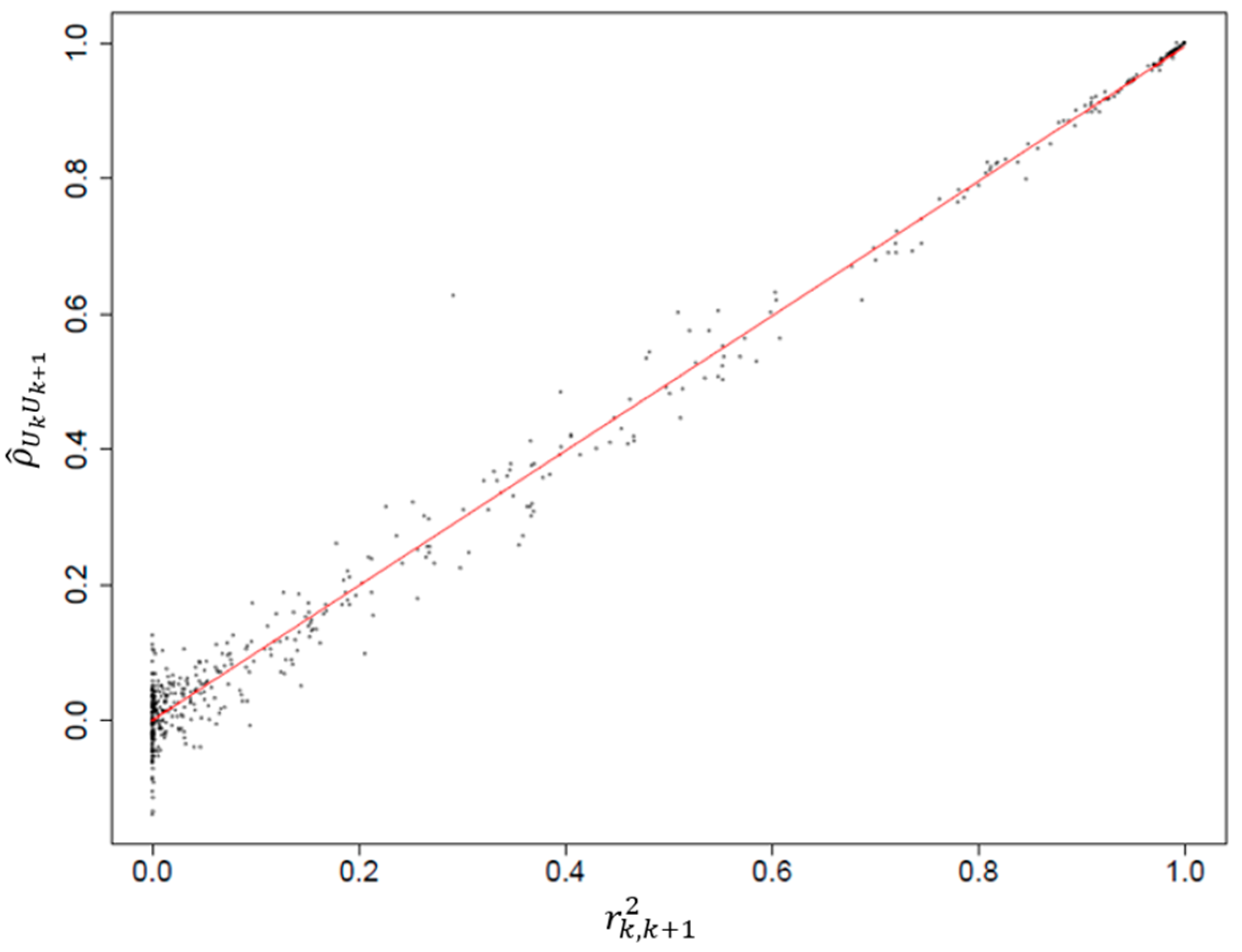
2.2. Empirical Pairwise Correlation of Tests

GWAS focuses on the identification of genetic variants associated with disease. SNPs, which consist of a single base pair variation in the DNA sequence, are the most commonly used genetic variants considered in such studies. Estimating the correlation between SNPs is crucial to understanding the genetic architecture of the trait under investigation. In this section, a method is proposed to estimate the correlation between SNPs via simulation. We evaluate genotype data on Chromosome 16 from the Wellcome Trust Case Control Consortium (WTCCC) study of Crohn’s disease, which included 1504 unaffected individuals. To preserve the correlation structure of the SNPs, a pair of haplotypes was randomly sampled for each individual. Individuals from the 1958 British birth cohort were randomly selected and assigned disease status based on the disease-associated SNP rs3789038. The analysis was repeated on 3000 replicates, each consisting of 1500 randomly drawn cases and 1500 controls, containing 14,292 SNPs each. Since 813 SNPs had no variations, only 13,479 SNPs were considered. To reduce the computation time, an arbitrary number of 1000 randomly selected SNPs were used to calculate the p-values for each single SNP test.

The random variable $U_k$ was defined as −log₁₀$\left(p_k\right)$, where the $p_k$ are the p-values obtained from the single SNP tests of association between disease and the kth SNP, $k$ = 1, …, $m$. Here, $m$ is the number of SNPs used to estimate the pairwise correlations between the tests, denoted as ${\rho }_{U_k,U_{k+1}}$ (see Section 2.1 for details). The estimated pairwise correlations based on pairs of alleles ($r_{k,k+1}^2$) were plotted, as shown in Figure 1. The results indicate a clear linear trend between ${\widehat{\rho }}_{U_k{,U}_{k+1}}$ and $r_{k,k+1}^2$, with an estimated slope of 0.996 when using linear least squares regression. These findings suggest that the correlation between test statistics can be reasonably estimated by the correlation between single SNP tests measured using $r_{k,k+1}^2$, providing important insights into the genetic structure of the trait of interest at the DNA sequence level. In addition, the variance of the data points increases when the correlation between SNP tests (${\widehat{\rho }}_{U_k,U_{k+1}}$) is close to 0. This is due to the fact that low correlation values make the estimation of the relationship between variables less stable and conversely for high correlation values. Hence, data points tend to cluster more closely together when the values of ${\widehat{\rho }}_{U_k{U}_{k+1}}$ and $r_{k,k+1}^2$ are close to one.

2.3. Distribution of −log₁₀(p-Values)

The established theoretical distribution of the transformed −log₁₀(p-value) obtained from a single SNP test serves as the basis for the development of an approach for bandwidth selection and the construction of thresholds.

Proposition 2.

Consider a statistical hypothesis test using a positive-valued test statistic $U$ with a continuous null distribution function $F$, where the null hypothesis is rejected for large values of $U$ and the corresponding p-value of the test can be calculated as $p=1-F\left(u\right)$. Under the null hypothesis, the distribution of $U_k$ is an exponential with parameter $\lambda =ln10$.

Proof. 

The probability integral transformation establishes that the transformation $p=1-F\left(u\right)$ is 1-1, and thus, $F\left(u\right)$ follows a uniform distribution on interval [0, 1]. Through the application of the change in the variable rule, the distribution of $p$ is also uniform on [0, 1]. Furthermore, it follows that the probability density function of $U$, denoted as $f\left(u\right)$, can be expressed as

$$f\left(u\right)=f\left(p\right)\left|\frac{dp}{du}\right|.$$

Since $f\left(p\right)$ = 1 and $\frac{dp}{du}$ = $-{10}^{-u}ln10$, we can write

$$\left|\frac{dp}{du}\right|=ln\left(10\right)e^{-uln10}\mathrm{for}u\ge 0,$$

which is the density for the exponential with parameter $\lambda =ln10$. □

The above proposition provides the mean and variance of $U_k=-{log}_{10}\left(p_k\right)$, where $p_k$ is the unobserved p-value from the kth single SNP test, for $k$ = 1, …,$m$. Specifically, it shows that the mean and variance of $U_k$ are $E\left(U_k\right)=\frac{1}{ln10}$ and $Var\left(U_k\right)=\frac{1}{{\left(ln10\right)}^2}$, respectively. Moreover, based on the results of the study in Section 2.1, the covariance of $U_k$ and $U_{k\prime }$ where $k\ne k\prime$, can be approximated as:

$${\sigma }_{U_k{U}_k\prime }\approx \frac{r_{kk\prime }^2}{{\left(ln10\right)}^2}$$

(2)

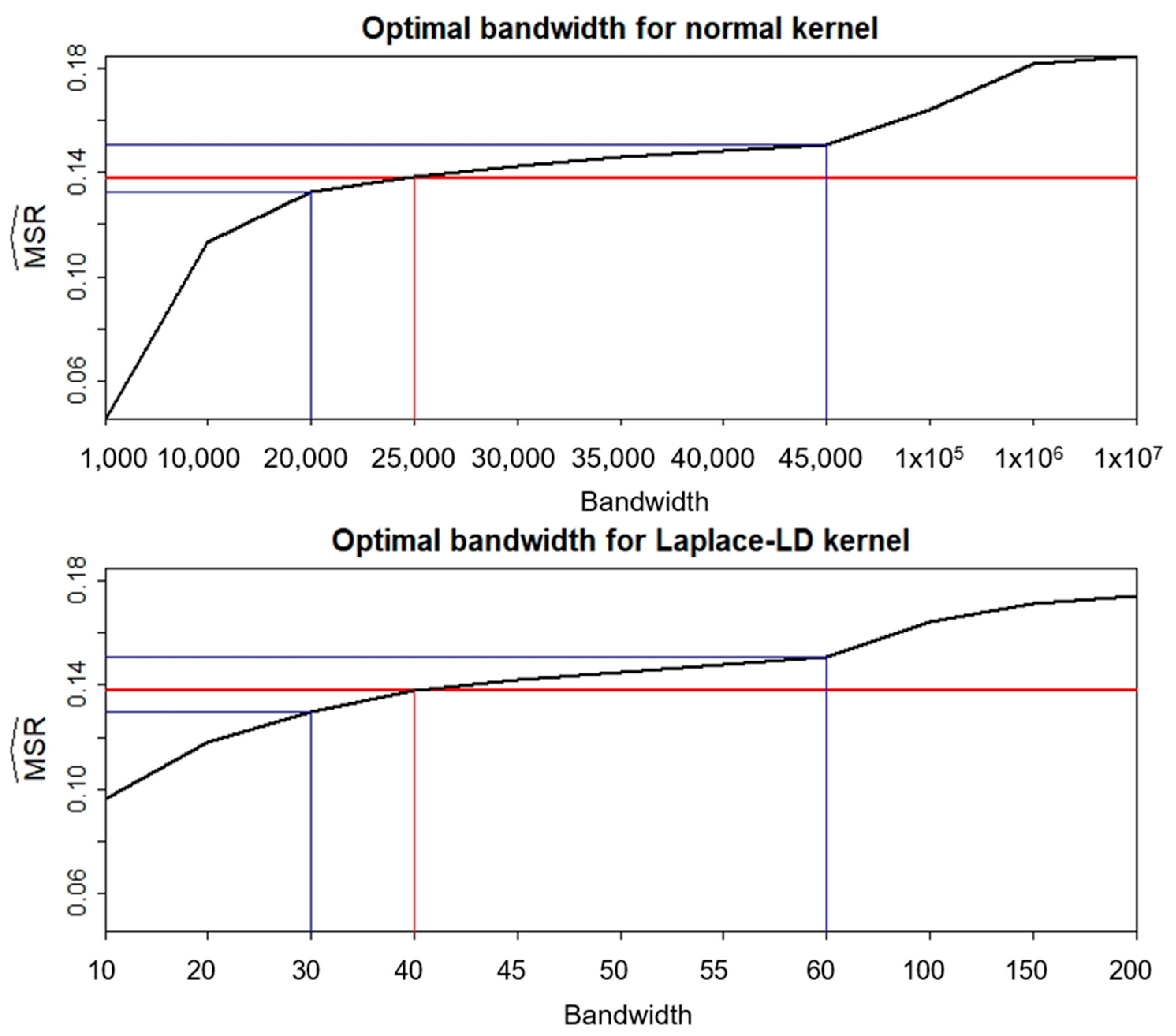
2.4. Optimal Bandwidth Selection Method

Consider the nonparametric regression model given by:

$$u_k=q\left(x_k\right)+{\epsilon }_k,$$

where $u_k$ represents −log₁₀$\left(p_k\right)$, $x_k$ represents the base pair position of the kth SNP, and the errors ${\epsilon }_k$, $k$ = 1, …, m, have a common variance. Methods for the bandwidth selection are here proposed based on fitting a curve that yields an acceptable estimate of the noise in the data under the null hypothesis, according to the mean of the squared residuals, denoted by $MSR$:

$$MSR=\frac{1}{m}{\sum }_{k=1}^m{\epsilon }_k^2.$$

In particular, a bandwidth $h$ can be selected such that it satisfies the condition:

$$\frac{1}{m}{\sum }_{k=1}^m{\left(u_k-{\widehat{u}}_k\right)}^2=E\left(MSR\right),$$

where ${\widehat{u}}_k$ is the fitted value of $u_k$. The average squared residuals for the fitted model are thus made equal to $E\left(MSR\right)$ through the selection of $h$.

In order to determine the expectation $E\left(MSR\right)$, we use the fact that $E\left({\epsilon }_k^2\right)={\sigma }_{{\epsilon }_k}^2$. Therefore,

$$E\left(MSR\right)=\frac{1}{m}{\sum }_{k=1}^m{\sigma }_{{\epsilon }_k}^2,$$

where ${\sigma }_{{\epsilon }_k}^2={\sigma }_{U_k}^2$ under the assumption that the $u_k$ are independent. It follows that the distribution of the −log₁₀(p-value) evaluated under the null hypothesis is given by

$$E\left(MSR\right)=\frac{1}{{\left(ln10\right)}^2}.$$

(3)

Yatchew [31] proposed a method for estimating the residual variance of the regression of $u$ on $x$, given by $s_d^2=\frac{1}{2n}{\sum }_{k=1}^{m-1}{\left(u_{k+1}-u_k\right)}^2$ when using the rearranged data as considered in the present work. Assuming $x_k$ is close to $x_{k+1}$, then $u_k\approx u_{k+1}$, and

$$s_d^2=\frac{1}{2m}{\sum }_{k=1}^{m-1}{\left(u_{k+1}-u_k\right)}^2=\frac{1}{2m}{\sum }_{k=1}^{m-1}{\left({\epsilon }_{k+1}-{\epsilon }_k\right)}^2.$$

(4)

By expanding Equation (4), therefore

$$s_d^2\approx \frac{1}{m}\sum _{k=1}^m{\epsilon }_k^2-\frac{1}{m}\sum _{k=1}^{m-1}{\epsilon }_k{\epsilon }_{k+1},$$

which, upon taking expectation, provides

$$E\left(s_d^2\right)\approx E\left(MSR\right)-\frac{1}{m}{\sum }_{k=1}^{m-1}E\left({\epsilon }_k{\epsilon }_{k+1}\right).$$

Substituting $E\left(MSR\right)$ using Equation (3) and using the fact that $E\left({\epsilon }_k\right)=0$ and $Cov\left({\epsilon }_k{,\epsilon }_{k+1}\right)=E\left({\epsilon }_k{\epsilon }_{k+1}\right)-E\left({\epsilon }_k\right)E\left({\epsilon }_{k+1}\right)$, then

$$E\left({\epsilon }_k{\epsilon }_{k+1}\right)=Cov\left({\epsilon }_k,{\epsilon }_{k+1}\right).$$

The term $E\left({\epsilon }_k{\epsilon }_{k+1}\right)$ can be evaluated using Equation (2), and the properties of the covariances are preserved under linear transformations. This gives

$$E\left({\epsilon }_k{\epsilon }_{k+1}\right)\approx \frac{r_{k,k+1}^2}{{\left(ln10\right)}^2}.$$

Therefore,

$$E\left(s_d^2\right)\approx \frac{1}{{\left(ln10\right)}^2}\left(1-\frac{1}{m}{\sum }_{k=1}^{m-1}{r}_{k,k+1}^2\right),$$

(5)

which justifies the selection of the optimal bandwidth $h$ satisfying the condition that the average squared residuals for the fitted model equal $s_d^2$.

The criterion in Equation (5) shows that $s_d^2$ can be interpreted as an estimate of the noise that is adjusted for the correlation structure of the neighboring SNPs.

2.5. Logistic Regression

Logistic regression is a powerful method and is suitable when the response variable is binary. It is an alternative to Pearson’s ${\chi }^2$ test and can be extended to multiple predictor variables. The relationship between the response and predictor variables is not linear (as in linear regression); instead, the logit function models their probabilities.

In this study, the response takes the value of 1 if an individual is a case and 0 if the individual is a control. For a given genotype $g_i$ for $n$ individuals, let ${\pi }_i$ be the conditional probability of the ith individual being a case. The logistic model for the relationship between ${\pi }_i$ and $g_i$ is:

$$logit\left({\pi }_i\right)={\beta }_0+{\beta }_1{g}_i,$$

where

$$logit\left({\pi }_i\right)=ln\left(\frac{{\pi }_i}{1-{\pi }_i}\right).$$

Using an additive genetic model, the probability of an individual being a case given the $D$ copies of the rare allele of the disease-associated SNP is:

$${\pi }_i=\frac{e^{{\beta }_0+{\beta }_{1}D}}{1+e^{{\beta }_0+{\beta }_{1}D}},$$

where the parameter ${\beta }_0$ is the baseline risk for the disease and ${\beta }_1$ is the gene effect or log-odds ratio.

In this study, the additive model for simulations is employed and assumes its application in the analysis of the WTCCC data. Nonetheless, for the single SNP analysis, a logistic regression model is utilized, which provides a more efficient but asymptotically equivalent alternative to Pearson’s ${\chi }^2$.

2.6. Kernel Regression

Kernel regression is a nonparametric regression method that estimates an arbitrary function of $x$, $q\left(x_k\right)$, using a kernel function, $K$. Unlike linear regression, the form of $q\left(·\right)$ is not known in advance. This approach can be seen as akin to nonlinear regression without explicitly stating the form of the function $q\left(·\right).$ The Nadaraya–Watson’s estimator [32] is a popular method that uses a kernel $K$ and bandwidth $h$ to estimate the fitted value of $u_k$ as follows:

$$\widehat{q}\left(x,h\right)=\frac{{\sum }_{k=1}^m{w}_k{u}_k}{{\sum }_{k=1}^m{w}_k}.$$

The weights $w_k$ are determined by applying the kernel function and are given by

$$w_k=\frac{K\left(\frac{x-x_k}{h}\right)}{{\sum }_{k=1}^{m}K\left(\frac{x-x_k}{h}\right)},k=1,\dots ,m.$$

Clearly, the magnitude of the weights is determined by the chosen value of the bandwidth $h$. The weights used in the present work depend on the distance between SNPs and not on their correlation, with those SNPs located closer to the kth SNP contributing more to the fitted value ${\widehat{u}}_k$. This assumption is reasonable, as SNPs that are physically closer to the disease-associated gene are more likely to be linked with it and, thus, themselves associated with the disease. The weights assigned to $u_k$ can be calculated using a normal kernel and a fixed bandwidth, as shown below:

$$w_k=\frac{e^{\frac{-1}{2}{\left(\frac{x-x_k}{h}\right)}^2}}{{\sum }_{k=1}^m{e}^{\frac{-1}{2}{\left(\frac{x-x_k}{h}\right)}^2}},k=1,\dots ,m.$$

However, since the correlation between the SNPs depends not only on their distance but also on other factors, it may not always be desirable to use this approach. To account for correlations in the test procedure, kernels based on the pairwise linkage disequilibrium (LD) between SNPs can be used. If a disease is caused by an unknown number of disease loci and a number of loci of known position can be calculated from the available data, then the markers with the largest amounts of LD will be closest to the disease loci, assuming that the LD distance relationship holds precisely within a genomic region [33].

To ensure that the weights are not linear, the Laplace-LD kernel can be used, where SNPs in strong LD with the kth SNP contribute substantially more to the fitted value ${\widehat{u}}_k$. The Laplace-LD kernel obtains its name from its similarity to the Laplace distribution; the corresponding weights can be calculated as follows:

$$w_k=\frac{e^{\frac{-1}{h\ast {LD}_k}}}{{\sum }_{k=1}^m{e}^{\frac{-1}{h\ast {LD}_k}}},k=1,\dots ,m,$$

where the value of $h>0$ determines the relative contributions.

3. Results

3.1. Simulation Results

The simulation study used the R programming suite [34] to analyze 14,292 SNPs located on Chromosome 16 within a dataset of 1504 controls obtained from the WTCCC. Following the exclusion of 813 SNPs with no observed variations, the analysis was carried out on the remaining 13,479 SNPs. These SNPs were subjected to the method described in Section 2.4 for the purpose of determining an appropriate bandwidth denoted as h. The criterion for the bandwidth selection was that the average squared residuals should be equal to $s_d^2$—an estimate of the noise—while accounting for the correlation with neighboring SNPs. A scatterplot of $s_d^2$ against the variance ${\widehat{\sigma }}^2={\sum }_{k=1}^m\left(u_k-\overline{u}\right)/\left(m-1\right)$ of the −log₁₀(p-value) estimated from the simulated data, assuming no genetic association (Figure 2), provides additional support for the proposed method. The estimated slope of the regression line was 0.74, indicating that $s_d^2$ slightly underestimates the true noise. This is, in fact, acceptable since the goal of the present work is to identify local structures in the data. Furthermore, determining the correlation between the estimated noise terms using $s_d^2$ and SNP correlation appreciably lowers the overall computational cost. The strong alignment of the data points along a straight line and their tight clustering reveal a strong relationship between the values of $s_d^2$ and ${\widehat{\sigma }}^2$, suggesting that the estimate is a reliable approximation.

To evaluate the efficiency of the proposed method, cases and controls were generated, assuming that the randomly selected SNP rs3789038 is located in gene HMOX2 on chromosome 16 (referred to as the disease-associated SNP). Cases were generated based on the disease model with probability:

$${\pi }_i=\frac{e^{{\beta }_0+{\beta }_{1}D}}{1+e^{{\beta }_0+{\beta }_{1}D}},$$

where $D$ is the number of copies of the rare allele in the disease-associated SNP and ${\beta }_1$ is the gene effect. Simulation studies for ${\beta }_1=$0.2 and 0.4, based on 3000 replicates (1500 cases and 1500 controls), indicated that both methods showed promise when using small gene effects and were therefore retained for further investigation of more than one causal SNP.

In order to determine the appropriate bandwidth values for the proposed method, the average value of $s_d^2$ based on 3000 replicates was calculated as ${\overline{s}}_d^2$ = 0.1380. The optimal bandwidth was then obtained by plotting the estimated $MSR$ for normal and Laplace-LD kernels with different bandwidths, as shown in Figure 3. The horizontal line represents the estimated ${\overline{s}}_d^2$ of the noise in 13,479 considered −log₁₀(p-values) obtained from the single SNP tests. The optimal bandwidth for the normal kernel was found to lie in the range of 20,000 to 45,000, with a value of roughly 25,000 determining approximately equal $MSR$ and $s_d^2$ values. For the Laplace-LD kernel, the optimal bandwidth was roughly 40, with values in the range of 30 to 60 producing similar $MSR$ values as with the normal kernel. Note that the bandwidth ranges are not centered around ${\overline{s}}_d^2$, consistently with the observation that $s_d^2$ underestimates the noise in the data.

Bandwidths of 20,000, 25,000, and 40,000 were used for the normal kernel, and 30, 40, and 50 were used for the Laplace-LD kernel. The results were compared with Bonferroni corrections ${\alpha }_{0.05}^{\prime }$, ${\alpha }_{0.01}^{\prime }$, and ${\alpha }_{0.001}^{\prime }$. In practice, identifying significant regions rather than significant SNPs for the disease might be relevant, as there is no guarantee that a disease-predisposing SNP will be identified in the GWAS. Disease regions consisting of the SNPs within 100,000 base pairs of the disease-associated SNPs were constructed. The estimated true positive (TP) rate is the number of times at least one of the two disease regions was detected out of the replicate runs, while the false positive (FP) rate is the number of SNPs found to be significant that are not in any of the disease regions.

Simulations of disease-associated SNPs with low and moderate correlations, with a gene effect size of 0.2 (Figure 4) and a gene effect size of 0.4 (Figure 5), show that increasing bandwidths led to higher TP and FP rates. The Laplace-LD kernel had similar FP rates as those obtained with Bonferroni corrections but had consistently higher TP rates. The plots of the TP rates for all SNPs were close to one, while the observed FP rates were less than the Bonferroni corrections.

The plots indicate consistently lower FP rates using the Laplace-LD kernel compared to the normal kernel. Figure 6 provides further insight, showing similarly strong signals of the disease-gene association at around 4 × 10⁶ base pairs and between 6 × 10⁶ and 8 × 10⁶ base pairs for both kernels.

The proposed methods offer notable advantages in terms of computational efficiency, particularly when compared with the single SNP analysis. The analysis presented in

Table 1. The time required to execute each simulation replicate for the methods.

Average Time Consume per Replicate	Method
3.5 min	Normal kernel, h = 25,000
4.1 min	Laplace-LD kernel, h = 40
6.0 min	Single SNP

illustrates that the normal and Laplace-LD kernels, as proposed, exhibit significantly reduced time requirements. These results are based on simulations conducted using the R version 4.1.0 on hardware featuring an Intel (R) Core (TM) i7-1255U processor.

3.2. Application to Real Data

The GWAS data from the WTCCC study were processed with the proposed methods for detecting significance. The dataset consists of 14,292 SNPs on Chromosome 16 from 2005 cases of Crohn’s disease and 3004 controls. Evidence of disease-gene association was reported by the WTCCC at SNP rs17221417, located on gene NOD2, with the significant region spanning 1,250,000 base pairs on either side of rs17221417. The normal and Laplace-LD kernels were applied with the chosen bandwidths $h$ = 40,000 and $h$ = 20, respectively, while accounting for the fact that $s_d^2$ is expected to underestimate the true noise in the data. The significant SNPs within the regions are listed in

Table 2. Significant SNPs from the WTCCC study of Crohn’s disease dataset on Chromosome 16 using the proposed methods.

Significant SNPs in Region 1	Method
rs1981760-rs11076540	Normal kernel
rs6500315-rs7199150 rs7186163-rs2066849 rs1981760-rs11076540 rs7205760	Laplace-LD kernel
Significant SNPs in Region 2
rs4471699 rs11644392 rs11863150	Normal kernel
rs11644392	Laplace-LD kernel

. Both methods detected a larger region (region 1) located at around 4.9 × 10⁷ base pairs and contained a cluster of 23 SNPs (rs1981760 to rs11076540) on gene NOD2. However, the region 2 detected, containing rs11644392 located within an intron at locus NR-002453.4, was not reported in the WTCCC study.

4. Discussion and Conclusions

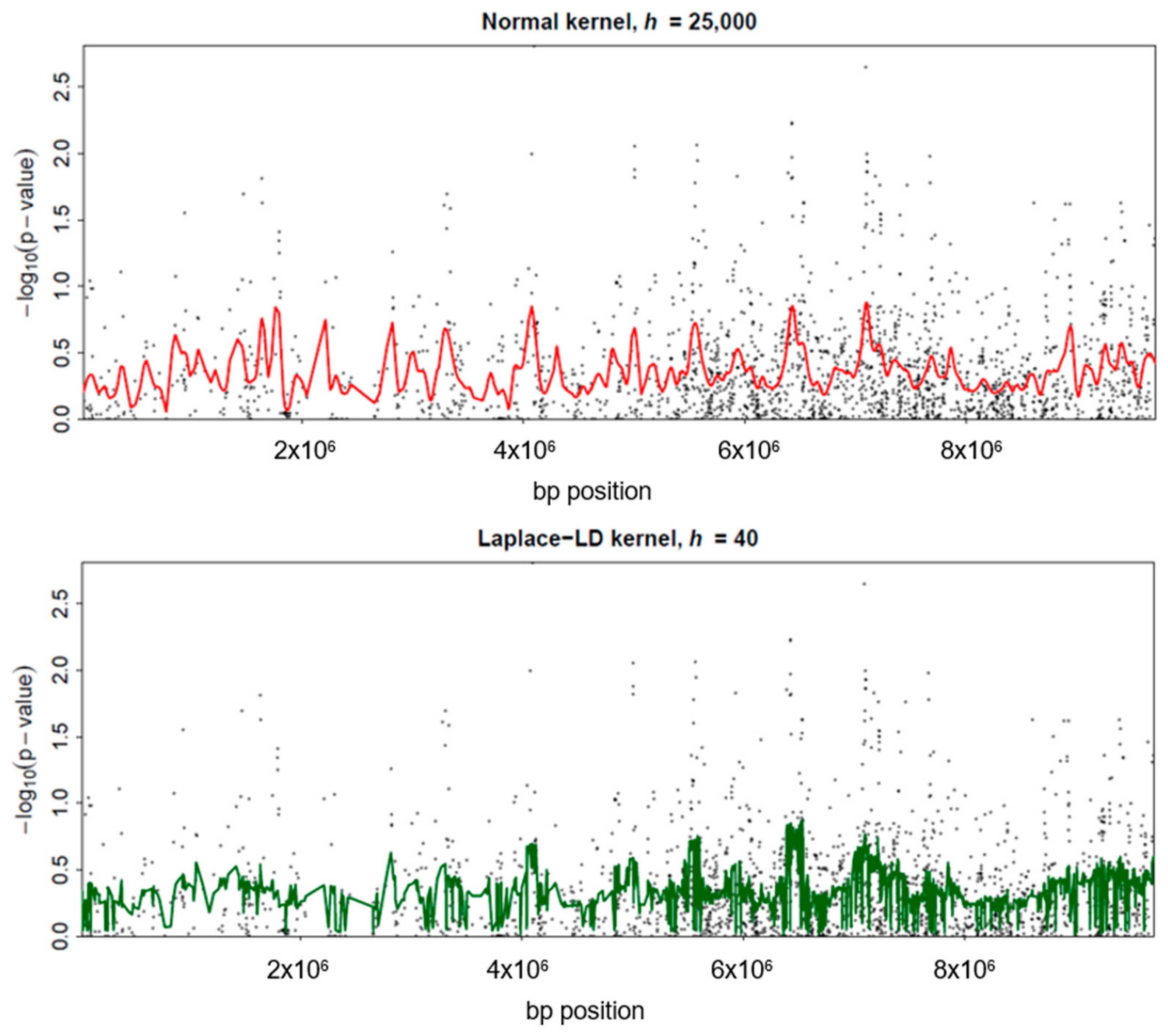
Given the evident need for advancements in the area of correlation structure and bandwidth selection in GWAS, the present work introduces a possible method to attack this problem and shows the potential of this approach. The method’s applicability to real genetic data, such as the WTCCC dataset with a specific focus on Crohn’s disease, has been showcased: the successful identification of clusters of disease-associated SNPs demonstrates the practical value of this approach in real-world genetic studies.

This study supports the applicability of this novel model-free method for effectively handling high-dimensional genetic data, with a focus on genome-wide association studies (GWAS). The approach capitalizes on the inherent correlations between tests, successfully mitigating the power loss typically associated with other multiple correction methods. By efficiently estimating the correlation structure and addressing the key aspects of kernel regression, the method described offers a robust result that can adjust to various datasets in GWAS.

There are promising directions for future research. A comprehensive simulation study could be undertaken to compare this new method’s performance with that of other existing approaches, such as the Nadaraya–Watson and local linear estimators. A comparative analysis would investigate the method’s adaptability and robustness across different genomic regions, including the examination of disease-associated SNPs close to chromosome boundaries.

Evaluation of these new methods, particularly concerning the normal and Laplace-LD kernels, highlights their computational efficiency and reliability. Future investigations should explore the optimal bandwidth selection process within the correlation structure, considering diverse scenarios and data types. Further refinement and improvement in the method’s applicability in the realm of high-dimensional genetic studies will ultimately advance our comprehension of complex diseases.

References

1. Uffelmann, E.; Huang, Q.Q.; Munung, N.S.; de Vries, J.; Okada, Y.; Martin, A.R.; Martin, H.C.; Lappalainen, T.; Posthuma, D. Genome-wide association studies. Nat. Rev. Methods Primers 2021, 1, 59. [Google Scholar] [CrossRef]
2. Li, Q.; Lin, J.; Racine, J.S. Optimal Bandwidth Selection for Nonparametric Conditional Distribution and Quantile Functions. J. Bus. Econ. Stat. 2013, 31, 57–65. [Google Scholar] [CrossRef]
3. Machiela, M.J.; Lindström, S.; Allen, N.E.; Haiman, C.A.; Albanes, D.; Barricarte, A.; Berndt, S.I.; Bueno-de-Mesquita, H.B.; Chanock, S.; Gaziano, M.J. Association of Type 2 Diabetes Susceptibility Variants with Advanced Prostate Cancer Risk in the Breast and Prostate Cancer Cohort Consortium. Am. J. Epidemiol. 2012, 176, 1121–1129. [Google Scholar] [CrossRef] [PubMed]
4. Visscher, P.M.; Wray, N.R.; Zhang, Q.; Sklar, P.; McCarthy, M.I.; Brown, M.A.; Yang, J. 10 Years of GWAS Discovery: Biology, Function, and Translation. Am. J. Hum. Genet. 2017, 101, 5–22. [Google Scholar] [CrossRef]
5. Sorić, B. Statistical discoveries and effect-size estimation. R. Stat. Soc. 1989, 84, 608–610. [Google Scholar] [CrossRef]
6. Halle, K.K.; Bakke, Ø.; Djurovic, S.; Bye, A.; Ryeng, E.; Wisløff, U.; Andreassen, O.A.; Langaas, M. Computationally efficient familywise error rate control in genome-wide association studies using score tests for generalized linear models. Scand. J. Stat. 2018, 47, 1090–1113. [Google Scholar] [CrossRef]
7. Sookkhee, S.; Kirdwichai, P.; Baksh, M.F. The efficiency of single SNP and SNP-set analysis in genome-wide association studies. Songklanakarin J. Sci. Technol. 2021, 43, 243–251. [Google Scholar] [CrossRef]
8. Mckenzie, D. An Overview of Multiple Hypothesis Testing Commands in Stata. Available online: https://blogs.worldbank.org/impactevaluations/overview-multiple-hypothesis-testing-commands-stata (accessed on 15 March 2023).
9. Sobota, R.S.; Shriner, D.; Kodaman, W.; Goodloe, R.; Zheng, W.; Gao, Y.; Edwards, T.; Amos, C.I.; Williams, S.M. Addressing Population-Specific Multiple Testing Burdens in Genetic Association Studies. Ann. Hum. Genet. 2015, 79, 136–147. [Google Scholar] [CrossRef]
10. Streiner, D.L.; Norman, G.R. Correction for Multiple Testing: Is there a resolution? Chest 2011, 140, 16–18. [Google Scholar] [CrossRef]
11. Zheng, J.; Richardson, T.G.; Millard, L.A.C.; Hemani, G.; Elsworth, B.L.; Raistrick, C.A.; Vilhjalmsson, B.; Neale, B.M.; Haycock, P.C.; Smith, F.D.; et al. PhenoSpD: An integrated toolkit for phenotypic correlation estimation and multiple testing correction using GWAS summary statistics. GigaScience 2018, 7, giy090. [Google Scholar] [CrossRef]
12. Segal, B.; Braun, T.; Elliott, M.; Jiang, H. Fast approximation of small p-values in permutation tests by partitioning the permutations. Biometrics 2018, 74, 196–206. [Google Scholar] [CrossRef] [PubMed]
13. Sondhi, A.; Rice, K.M. Fast permutation tests and related methods, for association between rare variants and binary outcomes. Ann. Hum. Genet. 2018, 82, 93–101. [Google Scholar] [CrossRef] [PubMed]
14. Hapfelmeier, A.; Hornung, R.; Haller, B. Efficient permutation testing of variable importance measures by the example of random forests. Comput. Stat. Data Anal. 2023, 181, 107689. [Google Scholar] [CrossRef]
15. Cinar, O.; Viechtbauer, W.A. Comparison of Methods for Gene-Based Testing That Account for Linkage Disequilibrium. Front. Genet. 2022, 13, 867724. [Google Scholar] [CrossRef]
16. Ping, Z.; Yang, Z.; Cheng, Q.; Liwei, Z.; Ruyang, Z.; Jianwei, G.; Jin, L.; Liya, L.; Feng, C. Statistical analysis for genome-wide association study. J. Biomed. Res. 2015, 29, 285–297. [Google Scholar] [CrossRef]
17. Johnson, R.C.; Nelson, G.W.; Troyer, J.L.; Lautenberger, J.A.; Kessing, B.D.; Winkler, C.A.; O’Brien, S.J. Accounting for multiple comparisons in a genome-wide association study (GWAS). BMC Genom. 2010, 11, 724. [Google Scholar] [CrossRef]
18. Eklund, A.; Andersson, M.; Knutsson, H. Fast Random Permutation Tests Enable Objective Evaluation of Methods for Single-Subject fMRI Analysis. Int. J. Biomed. Imaging 2011, 2011, 627947. [Google Scholar] [CrossRef]
19. Ekvall, M.; Höhle, M.; Käll, L. Parallelized calculation of permutation tests. Bioinformatics 2020, 36, 5392–5397. [Google Scholar] [CrossRef]
20. Foley, C.N.; Staley, J.R.; Breen, P.G.; Sun, B.B.; Kirk, P.D.W.; Burgess, S.; Howson, J.M.M. A fast and efficient colocalization algorithm for identifying shared genetic risk factors across multiple traits. Nat. Commun. 2021, 12, 764. [Google Scholar] [CrossRef]
21. Gao, X.; Becker, L.C.; Becker, D.M.; Starmer, J.D.; Province, M.A. Avoiding the high Bonferroni penalty in genome-wide association studies. Genet. Epidemiol. 2010, 34, 100–105. [Google Scholar] [CrossRef]
22. Meinshausen, N.; Maathuis, M.H.; Bühlmann, P. Asymptotic optimality of the Westfall-Young permutation procedure for multiple testing under dependence. Ann. Stat. 2011, 39, 3369–3391. [Google Scholar] [CrossRef]
23. Vilhjálmsson, B.J.; Yang, J.; Finucane, H.K.; Gusev, A.; Lindström, S.; Ripke, S.; Genovese, G.; Loh, P.R.; Bhatia, G.; Do, R.; et al. Modeling Linkage Disequilibrium Increases Accuracy of Polygenic Risk Scores. Am. J. Hum. Genet. 2015, 97, 576–592. [Google Scholar] [CrossRef] [PubMed]
24. The Wellcome Trust Case-Control Consortium. Genome-wide association study of 14,000 cases of seven common diseases and 3000 shared controls. Nature 2007, 447, 661–678. [Google Scholar] [CrossRef] [PubMed]
25. Atchadé, Y.F. A computational framework for empirical Bayes inference. Stat. Comput. 2011, 21, 463–473. [Google Scholar] [CrossRef]
26. Brewer, M.J. A Bayesian model for local smoothing in kernel density estimation. Stat. Comput. 2000, 10, 299–309. [Google Scholar] [CrossRef]
27. De Lima, M.S.; Atuncar, G.S. A Bayesian method to estimate the optimal bandwidth for multivariate kernel estimator. J. Nonparametric Stat. 2011, 23, 137–148. [Google Scholar] [CrossRef]
28. Cheng, T.; Gao, J.; Zhang, X. Nonparametric localized bandwidth selection for Kernel density estimation. Econom. Rev. 2019, 38, 733–762. [Google Scholar] [CrossRef]
29. Ferguson, T.S. A Course in Large Sample Theory, 1st ed.; Routledge: New York, NY, USA, 1996; pp. 39–43. [Google Scholar]
30. Pasaniuc, B.; Zaitlen, N.; Shi, H.; Bhatia, G.; Gusev, A.; Pickrell, J.; Hirschhorn, J.; Strachan, D.P.; Patterson, N.; Prince, A.L. Fast and accurate imputation of summary statistics enhances evidence of functional enrichment. Bioinformatics 2014, 30, 2906–2914. [Google Scholar] [CrossRef]
31. Yatchew, A. Nonparametric regression techniques in economics. J. Econ. Lit. 1998, 36, 669–721. Available online: http://www.jstor.org/stable/2565120 (accessed on 10 June 2021).
32. Nadaraya, E.A. On Estimating Regression. Theory Probab. Its Appl. 1964, 9, 141–142. [Google Scholar] [CrossRef]
33. Foulkes, A.S. Applied Statistical Genetics with R, 1st ed.; Springer: New York, NY, USA, 2009; pp. 65–96. [Google Scholar]
34. R Development Core Team. R: A Language and Environment for Statistical Computing; R Foundation Computing: Vienna, Austria, 2018; Available online: https://www.R-project.org (accessed on 10 June 2021).
Figure 1. Plot of the estimated correlation ρ ^ U k U k + 1 , measured by r k , k + 1 2 .
Mathematics 11 04710 g001
Figure 2. Scatter plot of s d 2 against the estimated variance σ ^ 2 of −log10(p-values).
Mathematics 11 04710 g002
Figure 3. Plots of the mean of M S R ^ against the bandwidth for normal and Laplace-LD kernels (horizontal middle line). The top and bottom horizontal lines illustrate the M S R ^ ranges for the bandwidth ranges of 20,000 to 45,000 for the normal kernel and 30 to 60 for the Laplace-LD kernel.
Mathematics 11 04710 g003
Figure 4. The ROC curve of false positives (FPs) and true positives (TPs) for detecting at least one SNP with (a) low correlation and (b) moderate correlation and gene effect size β 1 = 0.2.
Mathematics 11 04710 g004
Figure 5. The ROC curve of false positives (FPs) and true positives (TPs) for detecting at least one SNP with (a) low correlation and (b) moderate correlation and gene effect size β 1 = 0.4.
Mathematics 11 04710 g005
Figure 6. The fitted nonparametric regression curves against base pairs (bp) position using the normal and Laplace-LD kernels.
Mathematics 11 04710 g006