Relative Orderings of Modified Proportional Hazard Rate and Modified Proportional Reversed Hazard Rate Models

Abstract

In this paper, we identify several relative ordering properties of the modified proportional hazard rate and modified proportional reversed hazard rate models. For this purpose, we use two well-known relative orderings, namely the relative hazard rate ordering and the relative reversed hazard rate ordering. The investigation is to see how a relative ordering between two possible base distributions for the response distributions in these models is preserved when the parameters of the underlying models are changed. We will give some examples to illustrate the results and the conditions under which they are obtained. Numerical simulation studies have also been provided to examine the examples presented.

1. Introduction

The parameters of a distribution are typically considered to be real or perhaps vector values. In the literature, families of distributions are considered that are characterized by having a parameter that is itself a distribution function. These families are called semiparametric because they also contain a real parameter. Choosing the parameter that is first a distribution function is one possible way to use a semiparametric model. The underlying distribution is the formal name for this distribution function. In practice, the selection of an underlying distribution leads to the selection of a parametric model, but the selection is limited to families with the structure of the semiparametric model. Let F be a cumulative distribution function (cdf) of a lifetime unit with random life length $X_0$. In the context of reliability and survival analysis, this random variable usually stands as the random lifetime of a unit in a standard situation. Suppose that $d_{\mathit{\theta }}:[0,1]\mapsto [0,1]$ is a non-decreasing function for which $d_{\mathit{\theta }}\left(0\right)=0$, $d_{\mathit{\theta }}\left(1\right)=1$ where $\mathit{\theta }=({\theta }_1,\dots ,{\theta }_k)\in \Theta$ is a vector of unknown parameters, and $\Theta$ is the parameter space. Then, the random variable $X_1$ with the following cdf

$$F^{*}(t;\mathit{\theta })=d_{\mathit{\theta }}\left(F\left(t\right)\right).$$

(1)

is said to have a semiparametric model where F is the baseline distribution. In reliability, the random variable $X_1$ denotes the random lifetime of a unit in a fresh environment. The underlying distribution F might already have one or more parameters, in which case a semiparametric family might provide a way to include a new parameter, extending the family from which F originates. One can imagine that the standard families of the Gamma and Weibull distributions are derived from the exponential distribution via semiparametric families that include a second parameter. The Weibull and Gamma families can both be found as special cases of a three-parameter family using the same technique. The study of semiparametric families is therefore advantageous for two reasons: it provides a new understanding of traditional distribution families, and it offers strategies for extending families to make data fitting more flexible (see, e.g., Marshall and Olkin [1]).

The concept of the hazard rate (hr) function and also the concept of the reversed hazard rate (rhr) function play an important role in reliability and survival analysis. These quantities measure the instantaneous risk of failure of an aging technical system from the perspective of probability theory. Let X be the random lifetime of an aging technical system; then let the hr function of X, denoted by $h_X$, be defined as

$$h_X\left(t\right)=\underset{\delta \to 0^{+}}{lim}\frac{1}{\delta }P(X\le t+\delta |X>t)=\frac{f_X\left(t\right)}{{\overline{F}}_X\left(t\right)},$$

(2)

where $f_X$ is the probability density function (pdf) and ${\overline{F}}_X$ is the survival function (sf) associated with the random lifetime X. From (2) it can be seen that $h_X\left(t\right)$ measures the risk of failure of a unit or a technical system (with lifetime X) of age t in a very short interval in the immediate vicinity of the time t, for example, $(t,t+\delta ]$, in which $\delta$ is very close to zero. Therefore, the measure $h_X\left(t\right)$ as a function of t, the current age of a lifetime unit or technical system, is able to quantify the instantaneous risk of failure of the unit or technical system under consideration at any age (cf. Prentice and Kalbfleisch [2]). In some situations, a situation with previous failures can also be taken into account. For example, the actual inactivity time of a failed technical system at an inspection time t may not be known. In such cases, the rhr function is a useful measure to quantify the risk of past failures. The rhr of X, is denoted by ${\tilde{h}}_X$, defined as

$${\tilde{h}}_X\left(t\right)=\underset{\delta \to 0^{+}}{lim}\frac{1}{\delta }P(X>t-\delta |X\le t)=\frac{f_X\left(t\right)}{F_X\left(t\right)},$$

(3)

where $F_X$ is the cdf of X. It follows from (3) that ${\tilde{h}}_X\left(t\right)$ measures the risk of failure of a unit or technical system found to be inactive during an inspection at time t in a very short interval before time t, i.e., $(t-\delta ,t]$, so that $\delta$ is almost zero. Consequently, the quantity ${\tilde{h}}_X\left(t\right)$ is a function of t, the time at which the unit or technical system is inactive, can be used to measure the instantaneous risk of a past failure of the failed unit or technical system (see, for instance, Block et al. [3]).

Stochastic orders of random variables have long been a useful tool for making comparisons between probability distributions (see Müller and Stoyan [4], Shaked and Shanthikumar [5], Belzunce et al. [6], and Li and Li [7]). Basically, a stochastic order is a rule that defines the sense in which one stochastic variable is greater than or less than another. Some researchers used stochastic orders comparing distributions in terms of the magnitude of random variables to perform stochastic comparisons between semiparametric models, including those presented in Equations (5), (9) and (13) in Section 2. To this end, we quantify the effect of varying the parameters of the model on the variation of the response variables and, furthermore, the effect of changing the underlying distribution on changing the distribution of the response variables using several known stochastic orders. For example, in the context of the proportional hazard rate (PHR) model for the case where $\lambda$ is a random variable (frailty), Gupta and Kirmani [8] and subsequently Xu and Li [9] identified some stochastic ordering properties of the model. The PHR model has attracted the attention of many researchers in applied probability and statistics, for instance, see Psarrakos and Sordo [10], Sankaran and Kumar [11], Zhang et al. [12], Arnold et al. [13] and Kochar [14]. Considering the proportional reversed hazard rates (PRHR) model, Di Crescenzo [15] made some stochastic comparisons between two candidate distributions of the model that differ in their parameters. Kirmani and Gupta [16] derived some stochastic ordering results for the proportional odds rates (POR) model.

Recently, however, many researchers have focused on stochastic orders that compare lifetime distributions according to aging behavior, namely, the faster-aging stochastic orders. One of the key ideas in reliability theory and survival analysis is stochastic aging. It broadly outlines the pattern of aging/degradation of a system over time. Three different notions of aging are presented in the literature: positive aging, negative aging, and no aging. Positive aging implies a stochastically decreasing remaining lifetime of the system. Negative aging implies just the opposite. The system does not mature with time if there is no aging. To study different characteristics of system aging, various aging classes have been presented in the literature based on these three aging principles. The increasing failure rate (IFR), decreasing failure rate (DFR), increasing failure rate on average (IFRA), decreasing failure rate on average (DFRA), increasing likelihood ratio (ILR), and decreasing likelihood ratio (DLR) are among the frequently applied aging classes. The reader can consult Barlow and Proschan [17] and Lai and Xie [18] for further discussion on this topic. In addition to these ideas about aging, relative aging is a useful concept to use when studying system reliability. Relative aging is used to measure how a system changes over time relative to another system.

In real life, there are many situations where we deal with multiple systems of the same type (e.g., TVs from different manufacturers, CPUs from different brands, etc.). In these circumstances, we often encounter the following problem: how can we determine whether one system is aging faster than others over time? The idea of relative aging provides a compelling answer to this problem. When dealing with the crossover hazards/medium remaining life phenomena, another component of relative aging proves helpful. Many real-life situations involve this type of circumstance. For example, Pocock et al. [19] examined survival data on the effects of two different treatments on breast cancer patients and became aware of the phenomenon of crossover hazards. In addition, Champlin et al. [20] described several cases in which the superiority of one treatment over another lasted only for a short period of time. The above considerations suggest that increasing/decreasing hazard ratio models are a viable option in a variety of real-world scenarios. In fact, Kalashnikov and Rachev [21] have developed a concept of relative aging based on the monotonicity of the ratio of two hazard rate functions called the relative hazard rate order. This concept is known as faster hazard rate aging. Sengupta and Deshpande [22] presented another idea in a similar way based on the monotonicity of the ratio of two cumulative hazard rate functions. Rezaei et al. [23] proposed a relative order based on the ratio of the reversed hazard rates of two random lifetimes and called it the relative reversed hazard rate order. We will utilize the relative hazard rate order and, further, the relative reversed hazard rate order to compare models belonging to a recently introduced semiparametric model.

Let us assume that $X_0$ and $Y_0$ are two non-negative random variables with continuous distribution functions (cdfs) F and G, respectively. Let $X_1$ and $Y_1$ be two non-negative random variables whose cdfs are transformations of cdfs of $X_0$ and $Y_0$, respectively. In view of (1), suppose that $X_1$ and $Y_1$ follow cdfs $F^{*}(t;\mathit{\theta })=d_{\theta }\left(F\left(t\right)\right)$ and $G^{*}(t;\mathit{\theta })=d_{\theta }\left(G\left(t\right)\right)$, respectively. The function $d_{\mathit{\theta }}$ is called the distortion function and the cdfs $F^{*}(t;\mathit{\theta })$ and $G^{*}(t;\mathit{\theta })$ are called distorted distribution functions. These kinds of distributions, called also semiparametric distributions, have attracted the attention of many researchers in statistics, economics, actuarial studies and reliability (see, e.g., Navarro et al. [24], Navarro and Águila [25], Lando and Bertoli-Barsotti [26], Kayid and Al-Shehri [27] and Navarro and Pellerey [28]). From theoretical perspectives, the distribution of order statistics and the distribution of record values arisen from a sample from F follows the foregoing semiparametric model (see, e.g., Izadkhah et al. [29]). In practical studies, the baseline cdfs $F\left(t\right)$ and $G\left(t\right)$ represent two models in a population under a standard (reference) situation, for example, the model of the lifetime of an item under a controlled environment. The distorted distributions $F^{*}(t;\mathit{\theta })$ and $G^{*}(t;\mathit{\theta })$ then specify two altered models in a fresh environment, for instance, the lifetime of an item in a critical situation. One of the problems that has attracted the attention of researchers in applied probability is two study conditions under which

$$X_0{\le }_o{Y}_0⟹X_1{\le }_o{Y}_1,$$

(4)

where ${\le }_o$ denotes a certain stochastic order. The preservation property given in (4) states that a certain stochastic ordering relation between the baseline populations leads to the same stochastic ordering relation between the altered populations. In the context of many well-known semiparametric models, the implication in (4) has been studied in the literature (see, e.g., Di Crescenzo [15], Kirmani and Gupta [16] and Gupta and Gupta [30]). However, the studies conducted in this regard have so far only dealt with stochastic orders that take into account the magnitude of the stochastic order. The considered semiparametric families of distributions in the previously accomplished studies have also had a single parameter.

The aim of this work is to perform stochastic comparisons of two newly defined semiparametric models. Each of these models has two parameters. The stochastic orderings we consider here are two recent stochastic orderings that focus on the relative aging of two lifetime units, namely, the relative hazard rate ordering and the relative inverse hazard rate ordering. In particular, we compare the modified proportional hazard rate model (MPHR) and the modified proportional reversed hazard rate model (MPRHR), which correspond to the relative hazard rate ordering and the relative reverse hazard rate ordering. Specifically, the MPHR model is identified as a particular case of (1), such that $\mathit{\theta }=(\alpha ,\lambda )$, in which $\alpha >0$, $\lambda >0$ ($\overline{\alpha }=1-\alpha$) and

$$d_{\mathit{\theta }}\left(u\right)=\frac{1-{(1-u)}^{\lambda }}{1-\overline{\alpha }{(1-u)}^{\lambda }}.$$

The MPRHR model is also identified as a specific case of (1), so that $\mathit{\theta }=(\alpha ,\beta )$, where $\alpha >0$, $\beta >0$ and

$$d_{\mathit{\theta }}\left(u\right)=\frac{\alpha u^{\beta }}{1-\overline{\alpha }{u}^{\beta }}.$$

We consider random lifetimes $X_1$ and $Y_1$ with an MPHR distribution with hr functions $h_{X_1}$ and $h_{Y_1}$ and show that

$$\frac{h_{X_1}\left(t\right)}{h_{Y_1}\left(t\right)}\mathrm{is} \mathrm{non-decreasing} \mathrm{in}t\ge 0,$$

which shows that the unit or technical system with random life $X_1$ ages faster than the unit or technical system with random life $Y_1$. In parallel, we assume that if $X_1$ and $Y_1$ have an MPRHR distribution with rhr functions ${\tilde{h}}_{X_1}$ and ${\tilde{h}}_{Y_1}$, then under certain conditions,

$$\frac{{\tilde{h}}_{X_1}\left(t\right)}{{\tilde{h}}_{Y_1}\left(t\right)}\mathrm{is}\mathrm{non-increasing}\mathrm{in}t>0,$$

indicating that the unit or technical system with random life $X_1$ ages faster compared to the unit or technical system with random life $Y_1$.

The rest of the paper is organized as follows. In Section 2, we give some advanced preliminary considerations and auxiliary results. In Section 3, we consider the modified proportional hazard rate model for comparison in terms of the relative hazard rate order. In this section, we further consider the modified proportional reversed hazard rate model to give some ordering properties according to the relative reversed hazard rate order. In Section 4, some examples with numerical simulation studies are provided to show that the theorems are fulfilled. In Section 5, we conclude the paper with a more detailed summary and provide an outlook on possible future studies. In Appendix A, we gather the proofs of the main theorems of the paper and also insert four tables to report the results of the simulation studies.

2. Preliminaries

In this section we give some mathematical definitions of the notions that will be utilized in this paper. This section contains a description of well-known facts from probability theory. For a detailed review on mathematical reliability theory, for example, the reader can see Barlow and Proschan [31], Rykov et al. [32] and Rykov et al. [33]. In the literature, many semiparametric families of distributions have been introduced and studied. Among these models, some of them find their applicability in the context of lifetime events. The Cox’s PHR model is of the important and frequently used semiparametric family of distributions (see Cox [34]). For a review of the PHR model we refer the reader to Kumar and Klefsjö [35]. Let us consider the parameter $\lambda >0$, called the frailty parameter. Then the PHR model is defined as

$$\overline{F}(t;\lambda )={\overline{F}}^{\lambda }\left(t\right),t\ge 0,$$

(5)

where $\overline{F}(·;\lambda )$ is the survival function (sf) of the response random variable and $\overline{F}(·)$ is the baseline sf. Let $X_0$ have an absolutely cdf $F(·)$ with probability density function (pdf) $f(·).$ Then, the hr of $X_0$, an important reliability quantity in survival analysis, measures the instantaneous risk of failure of a device with lifetime $X_0$ at a certain age (t, say). The hr of $X_0$ for all $t\ge 0$ that fulfills $\overline{F}\left(t\right)>0$ is defined as follows:

$$h\left(t\right):=-\frac{d}{dt}ln\left(\overline{F}\left(t\right)\right)=\frac{f\left(t\right)}{\overline{F}\left(t\right)}.$$

(6)

It is well-known that h characterizes the underlying sf, $\overline{F}$, as follows:

$$\overline{F}\left(t\right)=exp\{-{\int }_0^{t}h\left(x\right)dx\}.$$

(7)

Suppose that $h(·;\lambda )$ is the hr function associated with the sf (5). Then, it is plainly seen that for every $t\ge 0$ for which $min(\overline{F\left(t\right)},\overline{F}(t;\lambda ))>0,$

$$h(t;\lambda )=\lambda \times h\left(t\right).$$

(8)

In contrast to the PHR model, the PRHR model was introduced by Gupta et al. [36]. We refer the reader to Gupta and Gupta [30] for further descriptions of the PRHR model. In the PRHR model, a positive parameter, $\beta$, called the resilience parameter, is considered. The PRHR model is then defined as

$$F(t;\beta )=F^{\beta }\left(t\right),t\ge 0,$$

(9)

in which $F(·;\beta )$ is the cdf of the response random variable and $F(·)$ is the baseline cdf or the underlying distribution function of the model. The rhr of $X_0$, another reliability quantity, measures the risk of failure of a device (with original lifetime $X_0$) in the past at a certain time point t at which the device is found to be inactive. The rhr of $X_0$ for all $t\ge 0$ when $F\left(t\right)>0$ is derived via the following relation:

$$\tilde{h}\left(t\right):=\frac{d}{dt}ln\left(F\left(t\right)\right)=\frac{f\left(t\right)}{F\left(t\right)}.$$

(10)

It has been verified that $\tilde{h}$ characterizes the underlying cdf, F, as below:

$$F\left(t\right)=exp\{-{\int }_t^{+\infty }\tilde{h}\left(x\right)dx\}.$$

(11)

Let us now assume that $\tilde{h}(·;\beta )$ is the rhr function of the distribution with the cdf (9). Then, it is readily realized for all $t\ge 0$ for which $min\left\{F\right(t),F(t;\beta \left)\right\}>0$ that

$$\tilde{h}(t;\beta )=\beta \times \tilde{h}\left(t\right).$$

(12)

Another reputable semiparametric family of distributions is the POR model (see, e.g., Marshall and Olkin [37]). This model is defined with cdf

$$F(t;\alpha )=\frac{F\left(t\right)}{1-\overline{\alpha }\overline{F}\left(t\right)};t,\alpha \in R^{+},\overline{\alpha }=1-\alpha ,$$

(13)

In some situations the following model is alternatively utilized:

$$F(t;\alpha )=\frac{\alpha F\left(t\right)}{1-\overline{\alpha }F\left(t\right)};t,\alpha \in R^{+},\overline{\alpha }=1-\alpha .$$

(14)

The POR model, also known as the Marshall–Olkin model, has been considered by Rykov et al. [33] in the context of sensitivity analysis. The odds rate function of $X_0$ measures the relative odds of the event $\{X_0>t\}$ in terms of the event $\{X_0\le t\}$, where t is some point in time. The odds rate function of $X_0$ for all $t\ge 0$ when $F\left(t\right)>0$ is defined as follows:

$$O{R}_0\left(t\right):=\frac{\overline{F}\left(t\right)}{F\left(t\right)}.$$

(15)

We assume that $OR(t;\alpha )=\frac{\overline{F}(t;\alpha )}{F(t;\alpha )}$ is the odds rate function of the distribution with the cdf (13). Then, it is easily verified for all $t\ge 0$ for which $min\left\{F\right(t),F(t;\alpha \left)\right\}>0$ that

$$OR(t;\alpha )=\alpha \times O{R}_0\left(t\right).$$

(16)

Balakrishnan et al. [38] utilized the PHR (resp., PRHR) model as a baseline model in (13) (resp., (14)) to propose two new models, referred to as the MPHR and MPRHR models, respectively.

Suppose that $X_0$ is a baseline random variable with survival function $\overline{F}$. Let $X_{11},\cdots ,X_{1n}$ be independent and identically distributed (i.i.d.) lifetimes of n components of a system with a common distribution function $F(·;\alpha ,\lambda )$. Then, $X_{11},\cdots ,X_{1n}$ are said to follow the MPHR model with tilt parameter $\alpha$, modified proportional hazard rate $\lambda$ and baseline survival function $\overline{F}$ (denoted as $MPHR(\alpha ;\lambda ;\overline{F})$) if and only if,

$$F(x;\alpha ,\lambda )=\frac{1-{\overline{F}}^{\lambda }\left(x\right)}{1-\overline{\alpha }{\overline{F}}^{\lambda }\left(x\right)};x,\lambda ,\alpha \in R^{+},\overline{\alpha }=1-\alpha .$$

(17)

For the case of $\alpha =1$, (17) simply reduces to the PHR model. The MPHR model in (17) includes some well-known distributions such as the extended exponential and extended Weibull distributions (Marshall and Olkin [1]), extended Pareto distribution (Ghitany [39]) and extended Lomax distribution (Ghitany et al. [40]).

On the other hand, suppose $X_1,\cdots ,X_n$ are i.i.d. lifetimes of n components of a system with a common distribution functions F. Then, $X_1,\cdots ,X_n$ are said to follow the MPRHR model with tilt parameter $\alpha$, modified proportional reversed hazard rate $\beta$ and baseline distribution function F (denoted as MPRHR $(\alpha ;\beta ;F)$) if and only if

$$F(x;\alpha ,\beta )=\frac{\alpha F^{\beta }\left(x\right)}{1-\overline{\alpha }{F}^{\beta }\left(x\right)};x,\beta ,\alpha \in R^{+},\overline{\alpha }=1-\alpha .$$

(18)

Note that the PRHR model is a sub-model of (18) when $\alpha =1$. In Table 1, we shall give a summary of the semiparametric models that are used in this paper together with the sf, the cdf and the pdf of the models.

Table 1. Summary of semiparametric models with their distributional characteristics.

Model	sf	cdf	pdf
POR	${\displaystyle \frac{\alpha \overline{F}\left(t\right)}{1-\overline{\alpha }\overline{F}\left(t\right)}}$	${\displaystyle \frac{F\left(t\right)}{1-\overline{\alpha }\overline{F}\left(t\right)}}$	${\displaystyle \frac{\alpha f\left(t\right)}{{(1-\overline{\alpha }\overline{F}\left(t\right))}^2}}$
PHR	${\overline{F}}^{\lambda }\left(t\right)$	$1-{\overline{F}}^{\lambda }\left(t\right)$	$\lambda {\overline{F}}^{\lambda -1}\left(t\right)f\left(t\right)$
PRHR	$1-F^{\beta }\left(t\right)$	$F^{\beta }\left(t\right)$	$\beta F^{\beta -1}\left(t\right)f\left(t\right)$
MPHR	${\displaystyle \frac{\alpha {\overline{F}}^{\lambda }\left(t\right)}{1-\overline{\alpha }{\overline{F}}^{\lambda }\left(t\right)}}$	${\displaystyle \frac{1-{\overline{F}}^{\lambda }\left(t\right)}{1-\overline{\alpha }{\overline{F}}^{\lambda }\left(t\right)}}$	${\displaystyle \frac{\lambda \alpha {\overline{F}}^{\lambda -1}\left(t\right)}{{(1-\overline{\alpha }{\overline{F}}^{\lambda }\left(t\right))}^2}f\left(t\right)}$
MPRHR	${\displaystyle \frac{1-F^{\beta }\left(t\right)}{1-\overline{\alpha }{F}^{\beta }\left(t\right)}}$	${\displaystyle \frac{\alpha F^{\beta }\left(t\right)}{1-\overline{\alpha }{F}^{\beta }\left(t\right)}}$	${\displaystyle \frac{\beta \alpha F^{\beta -1}\left(t\right)}{{(1-\overline{\alpha }{F}^{\beta }\left(t\right))}^2}f\left(t\right)}$

We assume that the random variables X and Y have distribution functions F and G, survival functions $\overline{F}=1-F$ and $\overline{G}=1-G$, density functions f and g, hazard rate functions $h_X=f/\overline{F}$ and $h_Y=g/\overline{G}$ and reversed hazard rate functions ${\tilde{h}}_X=f/F$ and ${\tilde{h}}_Y=g/G$, respectively. To compare the magnitude of random variables, some notions of stochastic orders are introduced below.

Definition 1.

Suppose that X and Y are two non-negative random variables that denote the lifetime of two systems. The random variable X is then said to be smaller than the random variable Y in the

(i)

usual stochastic order (denoted by $X{⪯}_{st}Y$) if

$$\overline{F}\left(x\right)\le \overline{G}\left(x\right)for allx\ge 0;$$

(ii)

hazard rate order (denoted by $X{⪯}_{hr}Y$ ) if

$$\frac{\overline{G}\left(x\right)}{\overline{F}\left(x\right)}is non-decreasing inx\ge 0,$$

or equivalently, if $h_X\left(x\right)\ge h_Y\left(x\right)$ for all $x\ge 0$;

(iii)

reversed hazard rate order (denoted by $X{⪯}_{rh}Y$) if

$$\frac{G\left(x\right)}{F\left(x\right)}is non-decreasing inx>0,$$

or equivalently, if ${\tilde{h}}_X\left(x\right)\le {\tilde{h}}_Y\left(x\right)$ for all $x>0$;

(iv)

likelihood ratio order (denoted by $X{⪯}_{lr}Y$) if

$$g\left(x\right)/f\left(x\right)is non-decreasing inx\ge 0;$$

(v)

relative hazard rate order (denoted by $X{⪯}_{c}Y$) if

$$\frac{h_X\left(x\right)}{h_Y\left(x\right)}is non-decreasing inx\ge 0;$$

(vi)

relative reversed hazard rate order (denoted by $X{⪯}_{b}Y$) if

$$\frac{{\tilde{h}}_X\left(x\right)}{{\tilde{h}}_Y\left(x\right)}is non-increasing inx\ge 0.$$

Some stochastic orders in Definition 1 are connected to each other. In this regard, $X{⪯}_{lr}Y$ implies $X{⪯}_{hr}Y$ and $X{⪯}_{lr}Y$ also implies $X{⪯}_{rh}Y$. Furthermore, $X{⪯}_{hr}Y$ gives $X{⪯}_{st}Y$ and $X{⪯}_{rh}Y$ yields $X{⪯}_{st}Y.$ For further relations and properties of the stochastic orders ${⪯}_{lr},{⪯}_{hr},{⪯}_{rh}$ and ${⪯}_{st}$, we refer the reader to Shaked and Shanthikumar [5]. For more descriptions of the relative order ${⪯}_c$, we refer the reader to Kalashnikov and Rachev [21] and Sengupta and Deshpande [22]. For further properties of the relative order ${⪯}_b$, the reader can see Rezaei et al. [23].

3. Main Results

In this section, we present the main results of the paper, which include two main preservation properties. The preservation property of the relative hazard rate order under the setting of the MPHR model is studied. The preservation property of the relative reversed hazard rate order under the setting of the MPRHR model is also investigated. The proofs of the main theorems are moved to Appendix A.

3.1. Results on Relative Orderings of MPHR Distributions

In this section, we obtain a relative ordering property in the MPHR model according to the relative hazard rate order. We will consider the MPHR model in two settings where two sets of parameters $\mathit{\alpha }=({\alpha }_1,{\alpha }_2)$ and $\mathit{\lambda }=({\lambda }_1,{\lambda }_2)$, which are possibly different, are assigned and the possibly different baseline sfs $\overline{F}$ and $\overline{G}$ are also taken into account. Finding conditions on $\mathit{\alpha }$ and $\mathit{\beta }$ and also conditions on $\overline{F}$ and $\overline{G}$ to establish the preservation of the relative hazard rate ordering property in the MPHR model is the main objective of this section.

Before stating the next result we introduce some notation. Let $X_0$ and $Y_0$ have pdfs f and g and sfs $\overline{F}$ and $\overline{G}$, respectively, and, further, $X_1\sim MPHR({\alpha }_1;{\lambda }_1;\overline{F})$ and $Y_1\sim MPHR({\alpha }_2;{\lambda }_2;\overline{G})$. Then, using (17), the sfs of $X_1$ and $Y_1$, which are denoted by $\overline{F}(x;{\alpha }_1,{\lambda }_1)$ and $\overline{G}(x;{\alpha }_2,{\lambda }_2)$, respectively, can be written as follows:

$$\overline{F}(x;{\alpha }_1,{\lambda }_1)=\frac{{\alpha }_1\times {\overline{F}}^{{\lambda }_1}\left(x\right)}{1-\overline{{\alpha }_1}{\overline{F}}^{{\lambda }_1}\left(x\right)}\mathrm{and}\overline{G}(x;{\alpha }_2,{\lambda }_2)=\frac{{\alpha }_2\times {\overline{G}}^{{\lambda }_2}\left(x\right)}{1-\overline{{\alpha }_2}{\overline{G}}^{{\lambda }_2}\left(x\right)}.$$

(19)

Now, let us denote by $f(·;{\alpha }_1,{\lambda }_1)$ and $g(·;{\alpha }_2,{\lambda }_2)$ the pdfs of $X_1$ and $Y_1$, which can be obtained by taking derivatives of the cdfs in (19) as follows:

$$f(x;{\alpha }_1,{\lambda }_1)=\frac{{\lambda }_1{\alpha }_1{\overline{F}}^{{\lambda }_1-1}\left(x\right)}{{(1-\overline{{\alpha }_1}{\overline{F}}^{{\lambda }_1}\left(x\right))}^2}f\left(x\right)\mathrm{and}g(x;{\alpha }_2,{\lambda }_2)=\frac{{\lambda }_2{\alpha }_2{\overline{G}}^{{\lambda }_2-1}\left(x\right)}{{(1-\overline{{\alpha }_2}{\overline{G}}^{{\lambda }_2}\left(x\right))}^2}g\left(x\right).$$

(20)

Appealing to (19) together with (20), the hazard rate function of $X_1$ and the hazard rate function of $Y_1$ are acquired as:

$$h(x;{\alpha }_1,{\lambda }_1)=\frac{h\left(x\right)}{\mathrm{\Phi }(\overline{F}\left(x\right);{\alpha }_1,{\lambda }_1)}\mathrm{and}s(x;{\alpha }_2,{\lambda }_2)=\frac{s\left(x\right)}{\Phi (\overline{G}\left(x\right);{\alpha }_2,{\lambda }_2)}$$

(21)

where $h(·)$ and $s(·)$ are the hazard rate functions of $X_0$ and $Y_0,$ respectively, and the function $\Phi (u;\alpha ,\lambda )$ is given by

$$\Phi (u;\alpha ,\lambda )=\frac{1}{\lambda }(1-\overline{\alpha }{u}^{\lambda }),u\in [0,1].$$

We define here two measures of the relative hazard rates of $Y_0$ and $X_0$ with hazard rate functions $s(·)$ and $h(·),$ respectively. Let us denote two limiting points of the hazard rate ratio $\frac{s\left(t\right)}{h\left(t\right)}$ as follows:

$${\eta }_0:=\underset{t\to 0^{+}}{lim}\frac{s\left(t\right)}{h\left(t\right)}\mathrm{and}{\eta }_1:=\underset{t\to +\infty }{lim}\frac{s\left(t\right)}{h\left(t\right)}.$$

Theorem 1.

Let $X_0$ and $Y_0$ have sfs $\overline{F}$ and $\overline{G}$, respectively. Let $X_1\sim MPHR({\alpha }_1;{\lambda }_1;\overline{F})$ and $Y_1\sim MPHR({\alpha }_2;{\lambda }_2;\overline{G}),$ where ${\alpha }_i\in [0,1]$ and ${\lambda }_i>0$ for every $i=1,2$. Let $M(\mathit{\alpha },\mathit{\lambda },{\eta }_0)\ge 0$ be a function of $\mathit{\alpha }=({\alpha }_1,{\alpha }_2)$, $\mathit{\lambda }=({\lambda }_1,{\lambda }_2)$ and ${\eta }_0$, such that

$$M(\mathit{\alpha },\mathit{\lambda },{\eta }_0):=\underset{u\in [0,1]}{sup}\left(\frac{u^{-{\lambda }_2{\eta }_0}-{\overline{\alpha }}_2}{u^{-{\lambda }_1}-{\overline{\alpha }}_1}\right).$$

If

$$\frac{{\overline{\alpha }}_2}{{\overline{\alpha }}_1}.\frac{{\lambda }_2}{{\lambda }_1}{\eta }_1\ge M(\mathit{\alpha },\mathit{\lambda },{\eta }_0)$$

then

$$X_0{⪯}_c{Y}_0\Rightarrow X_1{⪯}_c{Y}_1.$$

(22)

Remark 1.

In the context of Theorem 1, the obtained result is immediately followed when ${\alpha }_2\le 1$ and ${\alpha }_1\ge 1$. To prove this claim, note that if ${\alpha }_2\le 1$ and ${\alpha }_1\ge 1$, then, for all $t\ge 0$ and for every ${\lambda }_i>0,i=1,2$, one has

$$\overline{G}\left(t\right)\frac{{\Phi }^{\prime }(\overline{G}\left(t\right);{\alpha }_2,{\lambda }_2)}{\Phi (\overline{G}\left(t\right);{\alpha }_2,{\lambda }_2)}\le 0and\overline{F}\left(t\right)\frac{{\Phi }^{\prime }(\overline{F}\left(t\right);{\alpha }_1,{\lambda }_1)}{\Phi (\overline{F}\left(t\right);{\alpha }_1,{\lambda }_1)}\ge 0.$$

Therefore, the parenthetical statement on the right-hand side of the inequality given in (A1) is non-positive. Thus, it is straightforward that if ${\alpha }_2\le 1$, ${\alpha }_1\ge 1$ and $X_0{⪯}_c{Y}_0$, then $X_1{⪯}_c{Y}_1$. In this case, the additional supremum condition in Theorem 1 can be omitted.

The following theorem states another setting for the parameters of two MPHR distributions so that the result of Theorem 1 is obtained under a different condition.

Theorem 2.

Let $X_0$ and $Y_0$ have sfs $\overline{F}$ and $\overline{G}$, respectively. Let $X_1\sim MPHR({\alpha }_1;{\lambda }_1;\overline{F})$ and $Y_1\sim MPHR({\alpha }_2;{\lambda }_2;\overline{G}),$ where ${\alpha }_i\in (1,+\infty )$ and ${\lambda }_i>0$ for every $i=1,2$. Let $m(\mathit{\alpha },\mathit{\lambda },{\eta }_1)\ge 0$ be a function of $\mathit{\alpha }=({\alpha }_1,{\alpha }_2)$, $\mathit{\lambda }=({\lambda }_1,{\lambda }_2)$ and also ${\eta }_1$ such that

$$m(\mathit{\alpha },\mathit{\lambda },{\eta }_1):=\underset{u\in [0,1]}{inf}\left(\frac{u^{-{\lambda }_2{\eta }_1}-{\overline{\alpha }}_2}{u^{-{\lambda }_1}-{\overline{\alpha }}_1}\right).$$

If

$$\frac{{\alpha }_2-1}{{\alpha }_1-1}.\frac{{\lambda }_2}{{\lambda }_1}{\eta }_0\le m(\mathit{\alpha },\mathit{\lambda },{\eta }_1)$$

then

$$X_0{⪯}_c{Y}_0\Rightarrow X_1{⪯}_c{Y}_1.$$

(23)

3.2. Results on Relative Orderings of MPRHR Distributions

In this section, we investigate the relative reversed hazard rate ordering property in two MPRHR models with possibly different sets of parameters $(\mathit{\alpha },\mathit{\beta })$, where $\mathit{\alpha }=({\alpha }_1,{\alpha }_2)$ and $\mathit{\beta }=({\beta }_1,{\beta }_2)$, and also under possibly different baseline distributions F and G.

We start by introducing some notation. Let $X_0$ and $Y_0$ have pdfs f and g with underlying cdfs F and G, respectively. Let us assume that $X_1^{★}\sim MPRHR({\alpha }_1;{\beta }_1;F)$ and $Y_1^{★}\sim MPRHR({\alpha }_2;{\beta }_2;G)$ and denote them by $F^{★}(·;{\alpha }_1,{\beta }_1)$ and $G^{★}(·;{\alpha }_2,{\beta }_2)$. Then, using (18), we have

$$F^{★}(x;{\alpha }_1,{\beta }_1)=\frac{{\alpha }_1\times F^{{\beta }_1}\left(x\right)}{1-\overline{{\alpha }_1}{F}^{{\beta }_1}\left(x\right)}\mathrm{and}{G}^{★}(x;{\alpha }_2,{\beta }_2)=\frac{{\alpha }_2\times G^{{\beta }_2}\left(x\right)}{1-\overline{{\alpha }_2}{G}^{{\beta }_2}\left(x\right)}.$$

(24)

Using (24), the pdfs of $X_1^{★}$ and $Y_1^{★}$ (signified by $f^{★}(·;{\alpha }_1,{\beta }_1)$ and $g^{★}(·;{\alpha }_2,{\beta }_2)$) are acquired as below:

$$f^{★}(x;{\alpha }_1,{\beta }_1)=\frac{{\beta }_1\times {\alpha }_1\times F^{{\beta }_1-1}\left(x\right)}{{(1-\overline{{\alpha }_1}{F}^{{\beta }_1}\left(x\right))}^2}f\left(x\right)\mathrm{and}{g}^{★}(x;{\alpha }_2,{\beta }_2)=\frac{{\beta }_2\times {\alpha }_2\times G^{{\beta }_2-1}\left(x\right)}{{(1-\overline{{\alpha }_2}{G}^{{\beta }_2}\left(x\right))}^2}g\left(x\right).$$

(25)

By dividing the pdfs in (25) into the cdfs given in (24), the reversed hazard rate function of $X_1$ and the reversed hazard rate function of $Y_1$ are derived as follows:

$$\tilde{h}(x;{\alpha }_1,{\beta }_1)=\frac{\tilde{h}\left(x\right)}{\Psi (F\left(x\right);{\alpha }_1,{\beta }_1)}\mathrm{and}\tilde{s}(x;{\alpha }_2,{\beta }_2)=\frac{\tilde{s}\left(x\right)}{\Psi (G\left(x\right);{\alpha }_2,{\beta }_2)}$$

(26)

where $\tilde{h}(·)$ and $\tilde{s}(·)$ are the reversed hazard rate functions of $X_0$ and $Y_0,$ respectively, and further, the function $\Psi (u;\alpha ,\beta )$ is defined as

$$\Psi (u;\alpha ,\beta )=\frac{1}{\beta }(1-\overline{\alpha }{u}^{\beta }),u\in [0,1].$$

Now, let us define two measures of relative reversed hazard rates of $Y_0$ and $X_0$ having reverenced hazard rate functions $\tilde{s}(·)$ and $\tilde{h}(·),$ respectively. The limiting points of the reversed hazard rate ratio $\frac{\tilde{h}\left(t\right)}{\tilde{s}\left(t\right)}$ is as follows:

$${\eta }_0^{★}:=\underset{t\to 0^{+}}{lim}\frac{\tilde{h}\left(t\right)}{\tilde{s}\left(t\right)}\mathrm{and}{\eta }_1^{★}:=\underset{t\to +\infty }{lim}\frac{\tilde{h}\left(t\right)}{\tilde{s}\left(t\right)}.$$

Theorem 3.

Let $X_0$ and $Y_0$ have cdfs F and G, respectively. Let $X_1^{★}\sim MPRHR({\alpha }_1;{\beta }_1;F)$ and $Y_1^{★}\sim MPRHR({\alpha }_2;{\beta }_2;G),$ where ${\alpha }_i\in [0,1]$ and ${\beta }_i>0$ for every $i=1,2$. Suppose that $m^{★}(\mathit{\alpha },\mathit{\beta },{\eta }_1^{★})$, which is a non-negative function of $(\mathit{\alpha },\mathit{\beta },{\eta }_1^{★})$ is defined as

$$m^{★}(\mathit{\alpha },\mathit{\beta },{\eta }_1^{★}):=\underset{u\in [0,1]}{inf}\left(\frac{u^{-\frac{{\beta }_1}{{\eta }_1^{★}}}-{\overline{\alpha }}_1}{u^{-{\beta }_2}-{\overline{\alpha }}_2}\right).$$

If

$$\frac{{\overline{\alpha }}_1}{{\overline{\alpha }}_2}\times \frac{{\beta }_1}{{\beta }_2}\times {\eta }_0^{★}\le m^{★}(\mathit{\alpha },\mathit{\beta },{\eta }_1^{★})$$

then

$$X_0{⪯}_b{Y}_0\Rightarrow X_1^{★}{⪯}_b{Y}_1^{★}.$$

(27)

Remark 2.

In the setting of Theorem 3, the derived result can be acquired when ${\alpha }_2\le 1$ and ${\alpha }_1\ge 1$. To verify this claim, one needs to observe that if ${\alpha }_2\le 1$ and ${\alpha }_1\ge 1$, then, for all $t>0$ and for ${\beta }_i>0,i=1,2$, we have

$$F\left(t\right)\frac{{\Psi }^{\prime }(F\left(t\right);{\alpha }_1,{\beta }_1)}{\Psi (F\left(t\right);{\alpha }_1,{\beta }_1)}\ge 0andG\left(t\right)\frac{{\Psi }^{\prime }(G\left(t\right);{\alpha }_2,{\beta }_2)}{\Psi (G\left(t\right);{\alpha }_2,{\beta }_2)}\le 0.$$

Thus, the parenthetical statement on the right-hand side of the inequality given in (A7) is clearly non-negative. Hence, it is not hard to see that if ${\alpha }_2\le 1$, ${\alpha }_1\ge 1$ and $X_0{⪯}_b{Y}_0$, then $X_1^{*}{⪯}_b{Y}_1^{*}$. In this setting, the additional infimum condition in Theorem 3 can be removed.

In the next theorem, we obtain the result of Theorem 3 under different conditions.

Theorem 4.

Let $X_0$ and $Y_0$ follow cdfs F and G, respectively. Suppose that $X_1^{★}\sim MPRHR({\alpha }_1;{\beta }_1;F)$ and $Y_1^{★}\sim MPRHR({\alpha }_2;{\beta }_2;G),$ where ${\alpha }_i\in (1,+\infty )$ and ${\beta }_i>0$ for every $i=1,2$. Consider $M^{★}(\mathit{\alpha },\mathit{\beta },{\eta }_0^{★})$ as a non-negative function of $(\mathit{\alpha },\mathit{\beta },{\eta }_0^{★})$ defined as

$$M^{★}(\mathit{\alpha },\mathit{\beta },{\eta }_0^{★}):=\underset{u\in [0,1]}{sup}\left(\frac{u^{-{\beta }_1\times {\eta }_0^{★}}-{\overline{\alpha }}_1}{u^{-{\beta }_2}-{\overline{\alpha }}_2}\right).$$

If

$$\frac{{\alpha }_1-1}{{\alpha }_2-1}\times \frac{{\beta }_1}{{\beta }_2}\times {\eta }_1^{★}\ge M^{★}(\mathit{\alpha },\mathit{\beta },{\eta }_0^{★})$$

then

$$X_0{⪯}_b{Y}_0\Rightarrow X_1^{★}{⪯}_b{Y}_1^{★}.$$

(28)

4. Examples and Simulation Analysis

In this section, we provide examples to show that the results of Theorems 1–4 are fulfilled. We also present some numerical studies to verify that the theorems and examples are valid, as shown in a simulation analysis. The numerical computations are moved to Appendix A.

In the following example, we show that the result of Theorem 1 is applicable.

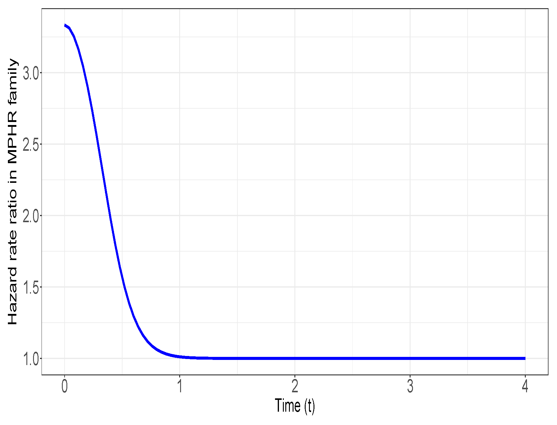
Example 1.

Let us write $X\sim W(c,d)$ when X follows the Weibull distribution with shape parameter c and scale parameter d, with $c,d>0$, having sf ${\overline{F}}_X\left(t\right)=exp(-{\left(dt\right)}^c),t\ge 0.$ Suppose that $X_0\sim W(3,1)$ and $Y_0\sim W(3,2)$. Assume that $X_1\sim MPHR({\alpha }_1;{\lambda }_1;\overline{F})$ and $Y_1\sim MPHR({\alpha }_2;{\lambda }_2;\overline{G})$ with ${\alpha }_1=0.8,{\alpha }_2=0.1,{\lambda }_1=10$ and ${\lambda }_2=1$ and, further, $\overline{F}\left(t\right)=exp(-t^3)$ and $\overline{G}\left(t\right)=exp(-8t^3).$ We can observe that $X_0$ and $Y_0$ have hrs $h\left(t\right)=3t^2$ and $s\left(t\right)=24t^2$. Therefore,

$$\frac{s\left(t\right)}{h\left(t\right)}=8,{\eta }_0={\eta }_1=8.$$

Hence, $X_0{⪯}_c{Y}_0.$ We can observe that

$$M(\mathit{\alpha },\mathit{\lambda },{\eta }_0):=\underset{u\in [0,1]}{sup}\left(\frac{u^{-8}-0.9}{u^{-10}-0.2}\right)=0.56812,$$

and, on the other hand, we can see that

$$\frac{{\overline{\alpha }}_2}{{\overline{\alpha }}_1}.\frac{{\lambda }_2}{{\lambda }_1}{\eta }_1=3.6.$$

Thus, obviously, $\frac{{\overline{\alpha }}_2}{{\overline{\alpha }}_1}.\frac{{\lambda }_2}{{\lambda }_1}>M(\mathit{\alpha },\mathit{\lambda },{\eta }_0)$, and using Theorem 1 we conclude that $X_1{⪯}_c{Y}_1$. In Figure 1, the graph of $\frac{s(t;{\alpha }_2,{\lambda }_2)}{s(t;{\alpha }_1,{\lambda }_1)}$ is plotted to exhibit that it is non-increasing in $t\in (0,4).$

Figure 1. Plot of the hazard rate ratio $\frac{s(t;{\alpha }_2,{\lambda }_2)}{h(t;{\alpha }_1,{\lambda }_1)}$ in Example 1 for ${\alpha }_1=0.8,{\alpha }_2=0.1,{\lambda }_1=10$ and ${\lambda }_2=1$ when $t\in (0,4)$.

We conduct here a simulation study to empirically ascertain that the result of Theorem 1 is valid. The parameters of the MPHR distributions are chosen exactly as in Example 1, i.e., $({\alpha }_1,{\lambda }_1)=(0.8,10)$ and $({\alpha }_2,{\lambda }_2)=(0.1,1)$, to fulfill the ordering result from the perspective of simulation analysis. We suppose that $X_0\sim W(3,1)$ and $Y_0\sim W(3,2)$, exactly as in Example 1. We assume X and Y follow MPHR distributions with cdfs $F(t;{\alpha }_1,{\lambda }_1)$ and $G(t;{\alpha }_2,{\lambda }_2)$ and right inverse functions $F^{-1}(u;{\alpha }_1,{\lambda }_1)$ and $G^{-1}(u;{\alpha }_2,{\lambda }_2)$, respectively. We also denote by $F^{-1}$ and $G^{-1}$, the right inverse functions associated with F and G, the cdfs of $X_0$ and $Y_0,$ respectively. On applying the runif function in R, we generate $u_1,u_2,\dots ,u_n\sim U(0,1)$, where $U(0,1)$ denotes the uniform distribution on $(0,1)$. We utilize the inverse transform technique to produce $x_i$ as

$$\begin{array}{cc}\hfill x_i& =F^{-1}(u_i;{\alpha }_1,{\lambda }_1)\hfill \\ \hfill & =F^{-1}\left({\displaystyle 1-\sqrt[{\lambda }_1]{\frac{1-u_i}{{\alpha }_1+u_i{\overline{\alpha }}_1}}}\right)\hfill \\ \hfill & {\displaystyle =\sqrt[3]{-\frac{1}{{\lambda }_1}\times ln\left(\frac{1-u_i}{{\alpha }_1+u_i{\overline{\alpha }}_1}\right)},i=1,2,\dots ,n,}\hfill \end{array}$$

by which n samples from $F(t;{\alpha }_1,{\lambda }_1)$ are generated when $({\alpha }_1,{\lambda }_1)=(0.8,10)$, i.e., $x_i\sim MPHR$$(0.8;10;\overline{F})$ with $\overline{F}\left(t\right)=exp(-t^3)$. In a similar manner, one can produce $y_i$ as

$$\begin{array}{cc}\hfill y_i& =G^{-1}(u_i;{\alpha }_2,{\lambda }_2)\hfill \\ \hfill & =G^{-1}\left({\displaystyle 1-\sqrt[{\lambda }_2]{\frac{1-u_i}{{\alpha }_2+u_i{\overline{\alpha }}_2}}}\right)\hfill \\ \hfill & {\displaystyle =\sqrt[3]{-\frac{8}{{\lambda }_2}\times ln\left(\frac{1-u_i}{{\alpha }_2+u_i{\overline{\alpha }}_2}\right)},i=1,2,\dots ,n,}\hfill \end{array}$$

which provides n samples from $G(t;{\alpha }_2,{\lambda }_2)$ where $({\alpha }_2,{\lambda }_2)=(0.1,1)$, i.e., $y_i\sim MPHR(0.1;1;\overline{G})$ in which $\overline{G}\left(t\right)=exp(-8t^3)$. Using the produced samples, we estimate $({\alpha }_1,{\lambda }_1)$ and $({\alpha }_2,{\lambda }_2)$ using the maximum likelihood method to obtain a maximum likelihood estimation (MLE) of $({\alpha }_i,{\lambda }_i)$, which is denoted by $({\widehat{\alpha }}_i,{\widehat{\lambda }}_i),i=1,2$. The estimations will be acquired by solving the likelihood equations. The MLE $({\widehat{\alpha }}_1,{\widehat{\lambda }}_1)$ is derived by solving the next system of equations in terms of $({\alpha }_1,{\lambda }_1):$

$$\left\{\begin{array}{cc}{\displaystyle \frac{n}{{\lambda }_1}-\sum _{i=1}^n{x}_i^3-2{\overline{\alpha }}_1\sum _{i=1}^n\frac{x_i^3{e}^{-{\lambda }_1{x}_i^3}}{(1-{\overline{\alpha }}_1\times e^{-{\lambda }_1{x}_i^3})}=0,}\hfill & \\ {\displaystyle \frac{n}{{\alpha }_1}-2\sum _{i=1}^n\frac{e^{-{\lambda }_1{x}_i^3}}{(1-{\overline{\alpha }}_1\times e^{-{\lambda }_1{x}_i^3})}=0.}\hfill & \end{array}\right.$$

(29)

The MLE $({\widehat{\alpha }}_2,{\widehat{\lambda }}_2)$ is also obtained by solving the equations based on $({\alpha }_2,{\lambda }_2)$:

$$\left\{\begin{array}{cc}{\displaystyle \frac{n}{{\lambda }_2}-8\sum _{i=1}^n{y}_i^3-16{\overline{\alpha }}_2\sum _{i=1}^n\frac{y_i^3{e}^{-8{\lambda }_2{y}_i^3}}{(1-{\overline{\alpha }}_2\times e^{-8{\lambda }_2{y}_i^3})}=0,}\hfill & \\ {\displaystyle \frac{n}{{\alpha }_2}-2\sum _{i=1}^n\frac{e^{-8{\lambda }_2{y}_i^3}}{(1-{\overline{\alpha }}_2\times e^{-8{\lambda }_2{y}_i^3})}=0.}\hfill & \end{array}\right.$$

(30)

To solve the systems of equations given in (29) and in (30), we used the package nleqslv in R. In Table A1 in Appendix A, we report the MLEs of the parameters of the MPHR model numerically under different sample sizes and also derive the amounts of MLE of $\frac{s(t;{\alpha }_2,{\lambda }_2)}{h(t;{\alpha }_1,{\lambda }_1)}$ for different selected ages t. It is shown that the estimated hazard rate ratio for the two choices made in Example 1 is non-increasing in t, as was expected.

The following example provides a situation where the result of Theorem 2 is applicable.

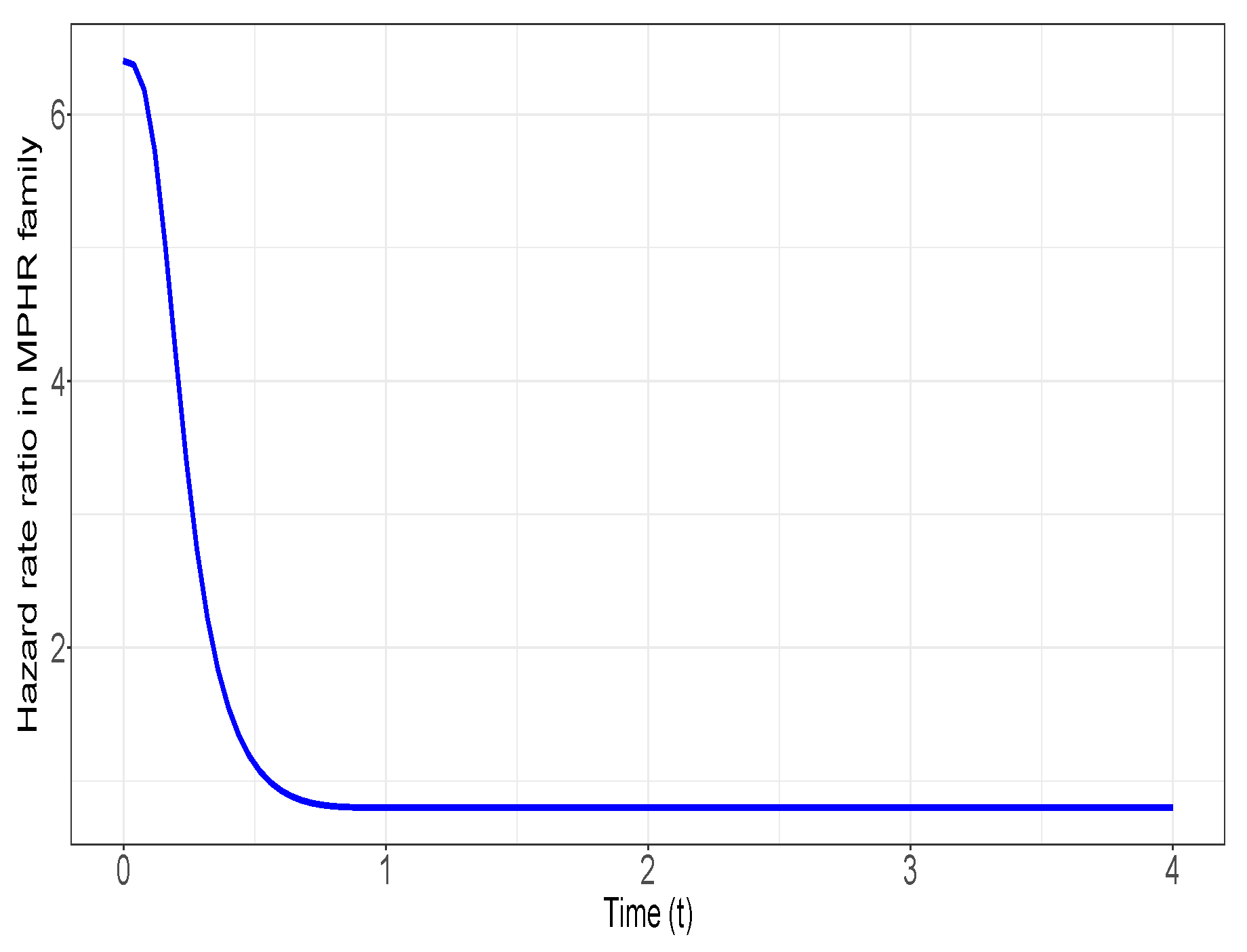
Example 2.

Suppose that $X_0$ follows a gamma distribution with sf $\overline{F}\left(t\right)=(1+3t)exp(-3t),t\ge 0$ and $Y_0$ has sf $\overline{G}\left(t\right)={(1+3t)}^{2}exp(-6t),t\ge 0.$ It is easily seen that the hrs of $X_0$ and $Y_0$ are $h\left(t\right)=\frac{9t}{1+3t}$ and $s\left(t\right)=\frac{18t}{1+3t}$, respectively. Therefore,

$${\eta }_0={\eta }_1=\frac{s\left(t\right)}{h\left(t\right)}=2.$$

Now, since $\frac{s\left(t\right)}{h\left(t\right)}$ is non-increasing in t, then $X_0{⪯}_c{Y}_0.$ We assume that $X_1\sim MPHR({\alpha }_1;{\lambda }_1;\overline{F})$ and $Y_1\sim MPHR({\alpha }_2;{\lambda }_2;\overline{G})$ with ${\alpha }_1=10,{\alpha }_2=3,{\lambda }_1=4$ and ${\lambda }_2=2$. It is observable that

$$m(\mathit{\alpha },\mathit{\lambda },{\eta }_1):=\underset{u\in [0,1]}{inf}\left(\frac{u^{-4}+2}{u^{-4}+9}\right)=0.3,$$

and, in parallel, it is seen that

$$\frac{{\alpha }_2-1}{{\alpha }_1-1}\times \frac{{\lambda }_2}{{\lambda }_1}{\eta }_0=\frac{2}{9}.$$

Therefore, clearly, $\frac{{\alpha }_2-1}{{\alpha }_1-1}\times \frac{{\lambda }_2}{{\lambda }_1}{\eta }_0<m(\mathit{\alpha },\mathit{\lambda },{\eta }_1)$, and thus, an application of Theorem 2 concludes that $X_1{⪯}_c{Y}_1$. In Figure 2, the graph of $\frac{s(t;{\alpha }_2,{\lambda }_2)}{s(t;{\alpha }_1,{\lambda }_1)}$ is plotted to indicate that this ratio is non-increasing in $t\in (0,4).$

Figure 2. Plot of the hazard rate ratio $\frac{s(t;{\alpha }_2,{\lambda }_2)}{h(t;{\alpha }_1,{\lambda }_1)}$ in Example 2 for ${\alpha }_1=10,{\alpha }_2=3,{\lambda }_1=4$ and ${\lambda }_2=2$ when $t\in (0,4)$.

As reported in Table A2 in Appendix A, the values of the MLEs of $({\alpha }_i,{\lambda }_i)$ are available under different sample sizes by simulating data from $MPHR({\alpha }_1;{\lambda }_1;\overline{F})$ and $MPHR({\alpha }_2;{\lambda }_2;\overline{G})$, with $({\alpha }_i,{\lambda }_i),i=1,2$ and $\overline{F}$ and $\overline{G}$ exactly as chosen in Example 2. We additionally report the values of the MLE of $\frac{s(t;{\alpha }_2,{\lambda }_2)}{h(t;{\alpha }_1,{\lambda }_1)}$ for some selected ages t. It is indicated that, for the two candidate models in Example 2, the estimated hazard rate ratio is non-increasing in t, as was claimed.

Next, we make use of Theorem 3 to show that the result is fulfilled.

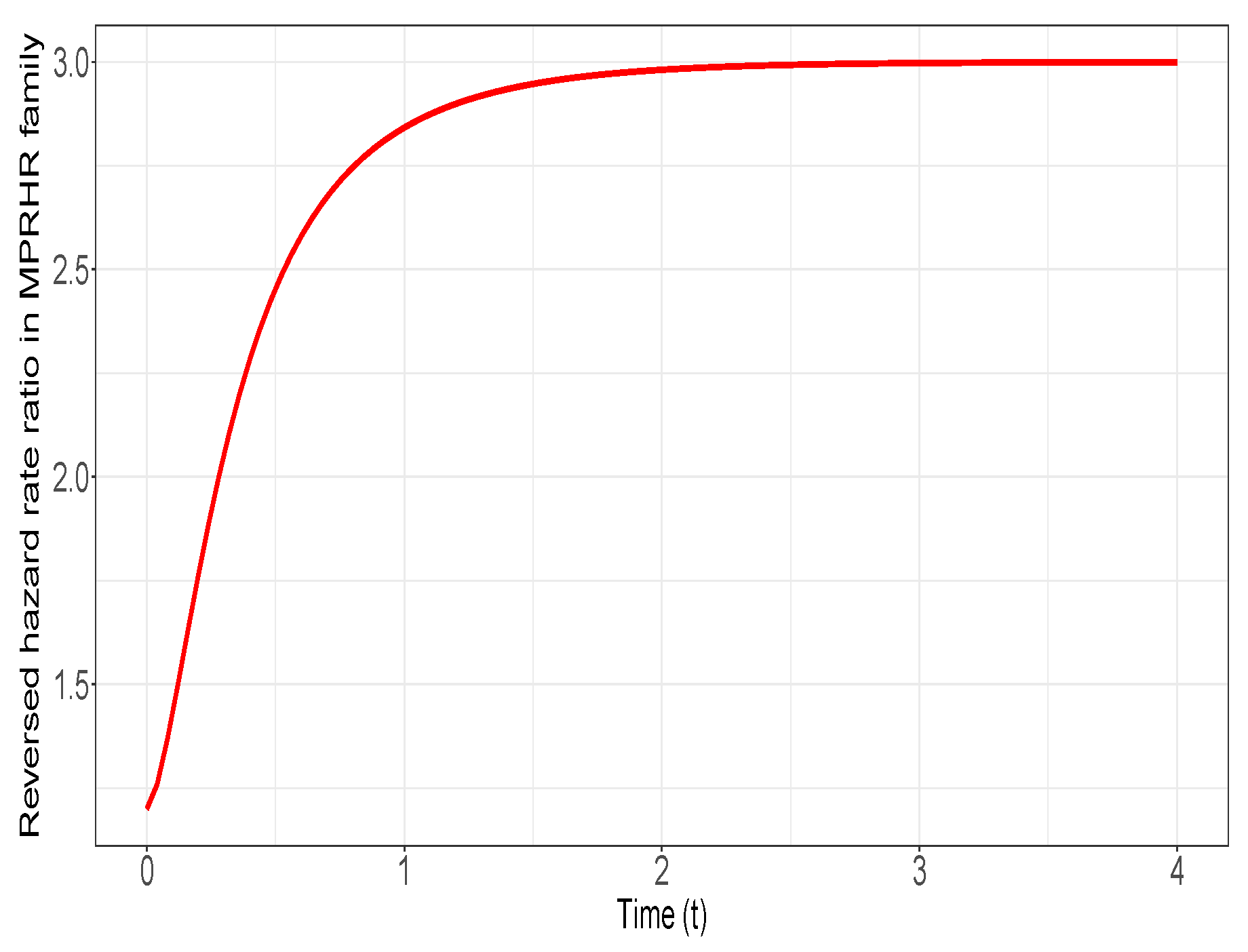
Example 3.

Let us assume $X\sim IW(c,d)$ whenever X has an inverse Weibull distribution with shape parameter c and scale parameter d, where $c>0$ and also $d>0$. Then, X has cdf $F_X\left(t\right)=exp(-{\left(\frac{d}{t}\right)}^c)$ for $t>0.$ We assume that $X_0\sim IW(2,1)$ and $Y_0\sim IW(2,3)$. Further, we suppose that $X_1^{*}\sim MPRHR({\alpha }_1;{\beta }_1;F)$ and $Y_1^{*}\sim MPRHR({\alpha }_2;{\beta }_2;G)$ with ${\alpha }_1=0.25, {\alpha }_2=0.5, {\beta }_1=2$ and ${\beta }_2=18$ so that $F\left(t\right)=exp(-{\left(\frac{3}{t}\right)}^2)$ is the cdf of $X_0$ and $G\left(t\right)=exp(-{\left(\frac{1}{t}\right)}^2).$ It can be readily shown that $X_0$ and $Y_0$ have rhrs $\tilde{h}\left(t\right)=\frac{2}{t^3}$ and $\tilde{s}\left(t\right)=\frac{18}{t^3}$, respectively. Thus,

$$\frac{\tilde{h}\left(t\right)}{\tilde{s}\left(t\right)}=\frac{1}{9},{\eta }_0^{★}={\eta }_1^{★}=\frac{1}{9}.$$

Consequently, $X_0{⪯}_b{Y}_0.$ One can easily check that

$$m^{*}(\mathit{\alpha },\mathit{\beta },{\eta }_1^{★}):=\underset{u\in [0,1]}{inf}\left(\frac{u^{-18}-0.75}{u^{-18}-0.5}\right)=0.5,$$

and, simultaneously, one has

$$\frac{{\overline{\alpha }}_1}{{\overline{\alpha }}_2}\times \frac{{\beta }_1}{{\beta }_2}{\eta }_0^{*}\simeq 0.00823.$$

Therefore, one realizes that $\frac{{\overline{\alpha }}_1}{{\overline{\alpha }}_2}\times \frac{{\beta }_1}{{\beta }_2}{\eta }_0^{*}<m^{*}(\mathit{\alpha },\mathit{\beta },{\eta }_1^{★})$, and using Theorem 3, we deduce that $X_1^{★}{⪯}_b{Y}_1^{★}$. In Figure 3, the graph of $\frac{\tilde{s}(t;{\alpha }_2,{\beta }_2)}{\tilde{h}(t;{\alpha }_1,{\beta }_1)}$ is exhibited to indicate that it is non-decreasing in $t\in (0,4).$

Figure 3. Plot of the reversed hazard rate ratio $\frac{\tilde{s}(t;{\alpha }_2,{\beta }_2)}{\tilde{h}(t;{\alpha }_1,{\beta }_1)}$ in Example 3 for ${\alpha }_1=0.25, {\alpha }_2=0.5, {\beta }_1=2$ and ${\beta }_2=18$ when $t\in (0,4)$.

We proceed now with another simulation study to examine the correctness of the result of Theorem 3. The parameters of the MPRHR distributions are selected as $({\alpha }_1,{\beta }_1)=(0.25,2)$ and $({\alpha }_2,{\beta }_2)=(0.5,18)$ and also assume that $X_0\sim IW(2,1)$ and $Y_0\sim IW(2,3)$, exactly as in Example 3. It is supposed that X and Y follow cdfs $F^{★}(t;{\alpha }_1,{\beta }_1)$ and $G^{★}(t;{\alpha }_2,{\beta }_2)$ and denote their right inverse functions by $F^{★,-1}(u;{\alpha }_1,{\beta }_1)$ and $G^{★,-1}(u;{\alpha }_2,{\beta }_2)$, respectively. We generate $u_1,u_2,\dots ,u_n\sim U(0,1)$. The inverse transform technique is implemented to simulate $x_i$ as

$$\begin{array}{cc}\hfill x_i& =F^{★,-1}(u_i;{\alpha }_1,{\beta }_1)\hfill \\ \hfill & =F^{-1}\left(\sqrt[-{\beta }_1]{\frac{{\alpha }_1}{u}+{\overline{\alpha }}_1}\right)\hfill \\ \hfill & =\sqrt{\frac{9{\beta }_1}{ln\left(\frac{{\alpha }_1}{u}+{\overline{\alpha }}_1\right)}},i=1,2,\dots ,n,\hfill \end{array}$$

from which one obtains n samples from $F^{★}(t;{\alpha }_1,{\lambda }_1)$ so that $({\alpha }_1,{\beta }_1)=(0.25,2)$, that is, $x_i\sim MPRHR(0.25;2;F)$ with $F\left(t\right)=exp(-\frac{9}{t^2})$. Analogously, to produce $y_i$, one has

$$\begin{array}{cc}\hfill y_i& =G^{★,-1}(u_i;{\alpha }_2,{\beta }_2)\hfill \\ \hfill & =G^{-1}\left(\sqrt[-{\beta }_2]{\frac{{\alpha }_2}{u}+{\overline{\alpha }}_2}\right)\hfill \\ \hfill & =\sqrt{\frac{{\beta }_1}{ln\left(\frac{{\alpha }_1}{u}+{\overline{\alpha }}_1\right)}},i=1,2,\dots ,n,\hfill \end{array}$$

through which n samples from $G^{★}(t;{\alpha }_2,{\beta }_2)$ are simulated in which $({\alpha }_2,{\beta }_2)=(0.5,18)$, i.e., $y_i\sim MPRHR(0.5;18;G)$, where $G\left(t\right)=exp(-\frac{1}{t^2})$. On the basis of the simulated samples, we want to find the MLEs of $({\alpha }_1,{\beta }_1)$ and $({\alpha }_2,{\beta }_2)$, which are denoted by $({\widehat{\alpha }}_i,{\widehat{\beta }}_i),i=1,2$. The MLE $({\widehat{\alpha }}_1,{\widehat{\beta }}_1)$ is derived by solving, with respect to $({\alpha }_1,{\beta }_1),$ the system of equations:

$$\left\{\begin{array}{cc}{\displaystyle \frac{n}{{\beta }_1}-9\sum _{i=1}^n\frac{1}{x_i^2}-18{\overline{\alpha }}_1\sum _{i=1}^n\frac{e^{-\frac{9{\beta }_1}{x_i^2}}}{(1-{\overline{\alpha }}_1\times e^{-\frac{9{\beta }_1}{x_i^2}})}=0,}\hfill & \\ {\displaystyle \frac{n}{{\alpha }_1}-2\sum _{i=1}^n\frac{e^{-\frac{9{\beta }_1}{x_i^2}}}{(1-{\overline{\alpha }}_1\times e^{-\frac{9{\beta }_1}{x_i^2}})}=0.}\hfill & \end{array}\right.$$

(31)

The MLE $({\widehat{\alpha }}_2,{\widehat{\beta }}_2)$ is also acquired by solving, in terms of $({\alpha }_2,{\beta }_2),$ the equations:

$$\left\{\begin{array}{cc}{\displaystyle \frac{n}{{\beta }_2}-\sum _{i=1}^n\frac{1}{y_i^2}-2{\overline{\alpha }}_2\sum _{i=1}^n\frac{e^{-\frac{{\beta }_2}{y_i^2}}}{(1-{\overline{\alpha }}_2\times e^{-\frac{{\beta }_2}{y_i^2}})}=0,}\hfill & \\ {\displaystyle \frac{n}{{\alpha }_2}-2\sum _{i=1}^n\frac{e^{-\frac{9{\beta }_2}{y_i^2}}}{(1-{\overline{\alpha }}_2\times e^{-\frac{{\beta }_2}{y_i^2}})}=0.}\hfill & \end{array}\right.$$

(32)

We gathered in Table A3 in Appendix A the values of the MLEs of the parameters of the MPRHR models under different sample sizes, and also obtain the MLE of $\frac{\tilde{s}(t;{\alpha }_2,{\beta }_2)}{\tilde{h}(t;{\alpha }_1,{\beta }_1)}$ for some t. It is acknowledged that the estimated reversed hazard rate ratio in the context of Example 3 is non-decreasing in t, as shown theoretically.

The following example is provided to examine the result of Theorem 4.

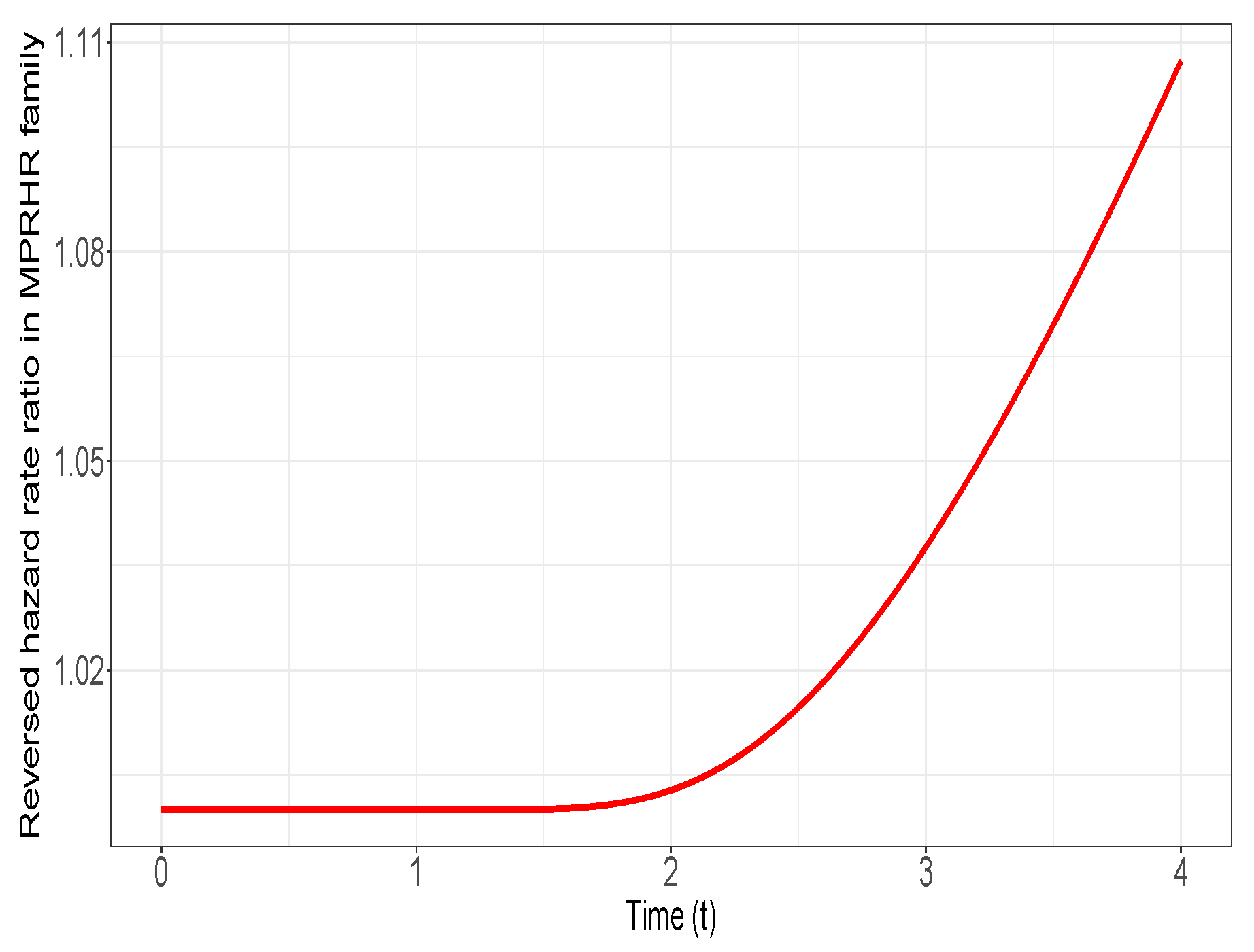
Example 4.

Let $X_0$ have cdf $F\left(t\right)={(1-exp(-\theta .t))}^{\frac{1}{3}},t\ge 0$ and let $Y_0$ have an exponential distribution with cdf $G\left(t\right)=1-exp(-\theta .t),t\ge 0$, where $\theta >0$ is a common parameter in F and G. Note that $\tilde{h}\left(t\right)=\frac{1}{3}.\tilde{s}\left(t\right)$ for all $t>0$, where $\tilde{h}$ is the rhr of $X_0$ and $\tilde{s}$ is the rhr of $Y_0$, respectively. Hence, ${\eta }_0^{★}={\eta }_1^{*}=\frac{1}{3},$ and also, clearly, $X_0{⪯}_b{Y}_0$. Suppose that $X_1^{*}\sim MPRHR({\alpha }_1,{\beta }_1,F)$ and $Y_1^{*}\sim MPRHR({\alpha }_2,{\beta }_2,G)$ such that ${\alpha }_1=5, {\alpha }_2=2, {\beta }_1=5$ and ${\beta }_2=2$. In view of the notations and definitions in Theorem 4, we have

$$M^{*}(\mathit{\alpha },\mathit{\beta },{\eta }_0^{*}):=\underset{u\in [0,1]}{sup}\left(\frac{u^{-\frac{5}{3}}+4}{u^{-2}+1}\right)=2.5,$$

and on the other hand, one has

$$\frac{{\alpha }_1-1}{{\alpha }_2-1}\times \frac{{\beta }_1}{{\beta }_2}\times {\eta }_1^{*}=\frac{10}{3}.$$

Thus, it is obvious that $\frac{{\alpha }_1-1}{{\alpha }_2-1}\times \frac{{\beta }_1}{{\beta }_2}\times {\eta }_1^{*}>M^{*}(\mathit{\alpha },\mathit{\beta },{\eta }_0^{*}).$ Therefore, Theorem 4 is applicable, which provides that $X_1^{*}{⪯}_b{Y}_1^{*}.$ In Figure 4, the curve of $\frac{\tilde{s}(t;{\alpha }_2,{\beta }_2)}{\tilde{h}(t;{\alpha }_1,{\beta }_1)}$ when $\theta =2,$ is plotted to verify that it is non-decreasing in $t\in (0,4).$

Figure 4. Plot of the reversed hazard rate ratio $\frac{\tilde{s}(t;{\alpha }_2,{\beta }_2)}{\tilde{h}(t;{\alpha }_1,{\beta }_1)}$ in Example 4 for ${\alpha }_1=5, {\alpha }_2=2, {\beta }_1=5$, ${\beta }_2=2$ and $\theta =2$ when $t\in (0,4)$.

We have listed in Table A4 in Appendix A the values of the MLEs of $({\alpha }_i,{\beta }_i),i=1,2$ under various sample sizes. We simulated data from $MPRHR({\alpha }_1;{\beta }_1;F)$ and $MPRHR({\alpha }_2;{\beta }_2;G)$ so that the parameters $({\alpha }_i,{\beta }_i),i=1,2$ together with the baseline cdfs F and G are chosen exactly as in Example 4. Further, we report the values of the MLE of $\frac{\tilde{s}(t;{\alpha }_2,{\beta }_2)}{\tilde{h}(t;{\alpha }_1,{\beta }_1)}$ for some selected times t. It is deduced that the estimated reversed hazard rate ratio of the two MPRHR distributions in Example 4 is non-decreasing in t. This proves the result of Theorem 4.

Remark 3.

The examples presented in this section show that the results obtained apply exclusively to exponential laws. The exponential family of distributions is a very important class of distributions. For example, in Bayesian statistics a prior distribution is multiplied by a likelihood function and then normalised to produce a posterior distribution. In the case of a likelihood that belongs to an exponential family, there exists a conjugate prior, which is often also in an exponential family. There are many standard lifetime distributions that belong to this family of distributions. And, in general, the move to semiparametric models is nothing new in statistics (see, for example, Bayesian methods, which can provide more fundamental results in reliability theory from this point of view). However, the two semiparametric models, namely, the MPHR model and MPRHR model, introduced by Balakrishnan et al. [38], have been found to be applied in different contexts, including reliability and survival analysis. This is because these models encompass three reputable classes of models, namely, the Marshall–Olkin or POR model, the PHR model and the PRHR model. These models have so many applications in reliability and survival analysis (see, e.g., Carree [41]).

5. Concluding Remarks

In this paper, we have examined two recently proposed semiparametric models, namely, the MPHR model and the MPRHR model. As shown by Balakrishnan et al. [38], these models include as special cases three important models in the literature, namely, the proportional hazard rate model, the proportional reversed hazard rate model and the proportional odds ratio model. Because these three models have found many applications in the literature so far and because they are available to the two newly defined semiparametric models, an analytical study of the latter models is needed because they cover and generalize the previous studies. The study of stochastic orderings for model comparisons has been carried out in the literature in various contexts, including reliability theory, survival analysis, actuarial analysis, risk theory, biostatistics and many other areas. Stochastic orderings are very useful potential tools for model analysis. For example, stochastic orders are very useful for detecting underestimation and overestimation problems in models. Stochastic orderings are usually recognized as tools for making inferences about models without data. The ordering properties of probability distributions reveal other aspects of the distribution or a family of distributions that can be used for various purposes.

The study conducted in this paper addresses situations in which there is a relative ordering property between two candidates from the MPHR family and, moreover, two candidates from the MPRHR family of semiparametric distributions. In general, the base distributions were assumed to be unknown but to satisfy a relative ordering property according to either the relative hazard rate order (${⪯}_c$) or the relative reversed hazard rate order (${⪯}_b$). It was assumed that the external parameters of the candidate models were generally different. Sufficient conditions were established for the conservation of the relative hazard rate order in the MPHR model and also for the conservation of the relative reversed hazard rate order in the MPRHR model. In the literature, for the preservation of the stochastic order in some scenarios, some stochastic orders are set as assumptions, which is a very strong condition. However, the conditions we found and presented in our work involve comparisons between two numbers, one of which is the supremum or infimum of a function and the other a function of the parameters of the models. With some examples we have shown that even very well-known standard statistical distributions that belong to the exponential family of distributions, such as the Weibull, Gamma or reversed Weibull distributions, can be used as the basic distribution in the MPHR and MPRHR model.

In many studies, different reliability models are considered with different intensities or hazard rate (reversed hazard rate) functions; moreover, there are even studies with compound and generalized intensities that have a discontinuity and atoms, as well as lattice distributions (see, for example, Kalimulina and Zverkina [42] and Kalimulina and Zverkina [43]). As can be seen from the graphs, the intensities considered in this paper are only continuous functions. This is a well-studied class of models (essentially exponential, generally a Weibull distribution). However, generalization of the results of this paper for more complicated intensities can be considered in future work.

In a future study, we can also consider stochastic comparisons in the MPHR and MPRHR models according to other stochastic orders, such as the likelihood ratio order (${⪯}_{lr}$), hazard rate order (${⪯}_{hr}$), reversed hazard rate order (${⪯}_{rh}$) and the usual stochastic order $\left({⪯}_{st}\right)$. In the context of the MPHR model, in view of (20), when $X_1$ and $Y_1$ follow the pdfs $f(x;{\alpha }_1,{\lambda }_1)$ and $g(x;{\alpha }_2,{\lambda }_2)$, respectively, then $X_0{⪯}_{lr}{Y}_0$ implies $X_1{⪯}_{lr}{Y}_1$ if

$$\frac{{\Phi }_1(\overline{G}\left(t\right);{\alpha }_2,{\lambda }_2)}{{\Phi }_1(\overline{F}\left(t\right);{\alpha }_1,{\lambda }_1)}\mathrm{is}\mathrm{non-decreasing}\mathrm{in}t\ge 0,$$

where ${\Phi }_1(u;\alpha ,\lambda ):=\frac{\lambda .\alpha .u^{\lambda -1}}{{(1-\overline{\alpha }.u^{\lambda })}^2}$. In addition, in the context of the MPHR model, when $X_1$ and $Y_1$ follow the sfs $\overline{F}(x;{\alpha }_1,{\lambda }_1)$ and $\overline{G}(x;{\alpha }_2,{\lambda }_2)$, respectively, as given in (19), then $X_0{⪯}_{st}{Y}_0$ implies $X_1{⪯}_{st}{Y}_1$ if

$${\Phi }_2(u;{\alpha }_1,{\lambda }_1)\le {\Phi }_2(u;{\alpha }_2,{\lambda }_2),\mathrm{for}\mathrm{all}u\in [0,1],$$

where ${\Phi }_2(u;\alpha ,\lambda )=\frac{\alpha .u^{\lambda }}{1-\overline{\alpha }.u^{\lambda }}$. In parallel, when the MPHR model is under consideration, as $X_1$ and $Y_1$ have hrs $h(x;{\alpha }_1,{\lambda }_1)$ and $s(x;{\alpha }_2,{\lambda }_2)$, respectively, as formulated in (21), then $X_0{⪯}_{hr}{Y}_0$ yields $X_1{⪯}_{hr}{Y}_1$ if

$$\underset{t\ge 0}{inf}\left(\frac{\Phi (\overline{G}\left(t\right);{\alpha }_2,{\lambda }_2)}{\Phi (\overline{F}\left(t\right);{\alpha }_1,{\lambda }_1)}\right)\ge 1,$$

where $\Phi$ is defined as in (21). On the other hand, concerning the MPRHR model, by appealing to (25) and assuming that $X_1^{*}$ and $Y_1^{*}$ have pdfs $f^{★}(x;{\alpha }_1,{\beta }_1)$ and $g^{*}(x;{\alpha }_2,{\beta }_2)$, respectively, then $X_0{⪯}_{lr}{Y}_0$ implies $X_1^{*}{⪯}_{lr}{Y}_1^{*}$ if

$$\frac{{\Psi }_1(G\left(t\right);{\alpha }_2,{\beta }_2)}{{\Psi }_1(F\left(t\right);{\alpha }_1,{\beta }_1)}\mathrm{is}\mathrm{non-decreasing}\mathrm{in}t\ge 0,$$

where ${\Psi }_1(u;\alpha ,\beta ):=\frac{\beta .\alpha .u^{\beta -1}}{{(1-\overline{\alpha }.u^{\beta })}^2}$. Moreover, by considering the MPRHR model, as $X_1^{*}$ and $Y_1^{*}$ follow cdfs $F^{*}(x;{\alpha }_1,{\beta }_1)$ and $G^{*}(x;{\alpha }_2,{\beta }_2)$, respectively, as provided in (24), then $X_0{⪯}_{st}{Y}_0$ implies $X_1^{*}{⪯}_{st}{Y}_1^{*}$ if

$${\Psi }_2(u;{\alpha }_1,{\beta }_1)\ge {\Psi }_2(u;{\alpha }_2,{\beta }_2),\mathrm{for}\mathrm{all}u\in [0,1],$$

where ${\Psi }_2(u;\alpha ,\beta )=\frac{\alpha .u^{\beta }}{1-\overline{\alpha }.u^{\beta }}$. Furthermore, when the MPRHR model is regarded, so that $X_1^{★}$ and $Y_1^{*}$ have rhrs $\tilde{h}(x;{\alpha }_1,{\beta }_1)$ and $\tilde{s}(x;{\alpha }_2,{\beta }_2)$, respectively, as written in (26), then $X_0{⪯}_{rh}{Y}_0$ yields $X_1^{*}{⪯}_{rh}{Y}_1^{*}$ if

$$\underset{t\ge 0}{sup}\left(\frac{\Psi (G\left(t\right);{\alpha }_2,{\beta }_2)}{\Psi (F\left(t\right);{\alpha }_1,{\beta }_1)}\right)\ge 1,$$

in which $\Psi$ is defined earlier in equations (26). The analogous study can also be carried out in the context of other stochastic orders such as the dispersive order, star order and super-additive order.

References

1. Marshall, A.W.; Olkin, I. Life Distributions; Springer: New York, NY, USA, 2007; Volume 13. [Google Scholar]
2. Prentice, R.L.; Kalbfleisch, J.D. Hazard rate models with covariates. Biometrics 1979, 1979, 25–39. [Google Scholar] [CrossRef]
3. Block, H.W.; Savits, T.H.; Singh, H. The reversed hazard rate function. Probab. Eng. Infor. Sci. 1998, 12, 69–90. [Google Scholar] [CrossRef]
4. Müller, A.; Stoyan, D. Comparison Methods for Stochastic Models and Risks; John Willey and Sons. Inc.: New York, NY, USA, 2002. [Google Scholar]
5. Shaked, M.; Shanthikumar, J.G. (Eds.) Stochastic Orders; Springer: New York, NY, USA, 2007. [Google Scholar]
6. Belzunce, F.; Riquelme, C.M.; Mulero, J. An Introduction to Stochastic Orders; Academic Press: Cambridge, MA, USA, 2015. [Google Scholar]
7. Li, H.; Li, X. Stochastic orders in reliability and risk. In Honor of Professor Moshe Shaked; Springer: New York, NY, USA, 2013. [Google Scholar]
8. Gupta, R.C.; Kirmani, S.N.U.A. Stochastic comparisons in frailty models. J. Stat. Plan. Inference 2006, 136, 3647–3658. [Google Scholar] [CrossRef]
9. Xu, M.; Li, X. Negative dependence in frailty models. J. Stat. Plan. Inference 2008, 138, 1433–1441. [Google Scholar] [CrossRef]
10. Psarrakos, G.; Sordo, M.A. On a family of risk measures based on proportional hazards models and tail probabilities. Insur. Math. Econ. 2019, 86, 232–240. [Google Scholar] [CrossRef]
11. Sankaran, P.G.; Dileep Kumar, M. Reliability properties of proportional hazards relevation transform. Metrika 2019, 82, 441–456. [Google Scholar] [CrossRef]
12. Zhang, M.; Lu, B.; Yan, R. Ordering results of extreme order statistics from dependent and heterogeneous modified proportional (reversed) hazard variables. Aims Math. 2021, 6, 584–606. [Google Scholar] [CrossRef]
13. Arnold, B.C.; Martínez-Flórez, G.; Gxoxmez, H.W. Bivariate Proportional Hazard Models: Structure and Inference. Symmetry 2022, 14, 2073. [Google Scholar] [CrossRef]
14. Kochar, S. Dependence comparisons of order statistics in the proportional hazards model. Probab. Eng. Infor. Sci. 2022, 2022, 730–736. [Google Scholar] [CrossRef]
15. Di Crescenzo, A. Some results on the proportional reversed hazards model. Stat. Probab. Lett. 2000, 50, 313–321. [Google Scholar] [CrossRef]
16. Kirmani, S.N.U.A.; Gupta, R.C. On the proportional odds model in survival analysis. Ann. Inst. Stat. Math. 2001, 53, 203–216. [Google Scholar] [CrossRef]
17. Barlow, R.E.; Proschan, F. Statistical Theory of Reliability and Life Testing: Probability Models; Holt, Rinehart and Winston: New York, NY, USA, 1975; Volume 1. [Google Scholar]
18. Lai, C.D.; Xie, M. Stochastic Ageing and Dependence for Reliability; Springer Science and Business Media: Berlin/Heidelberg, Germany, 2006. [Google Scholar]
19. Pocock, S.J.; Gore, S.M.; Keer, G.R. Long-term survival analysis: The curability of breast cancer. Stat. Med. 1982, 1, 93–104. [Google Scholar] [CrossRef] [PubMed]
20. Champlin, R.; Mitsuyasu, R.; Elashoff, R.; Gale, R.P. Recent Advances in Bone Marrow Transplantation; Gale, R.P., Ed.; UCLA Symposia on Molecular and Cellular Biology: New York, NY, USA, 1983; Volume 7, pp. 141–158. [Google Scholar]
21. Kalashnikov, V.V.; Rachev, S.T. Characterization of queueing models and their stability. In Probability Theory and Mathematical Statistics; VNU Science Press: Amsterdam, The Netherlands, 1986; Volume 2, pp. 37–53. [Google Scholar]
22. Sengupta, D.; Deshpande, J.V. Some results on the relative ageing of two life distributions. J. Appl. Probab. 1994, 31, 991–1003. [Google Scholar] [CrossRef]
23. Rezaei, M.; Gholizadeh, B.; Izadkhah, S. On relative reversed hazard rate order. Commun.-Stat.-Theory Methods 2015, 44, 300–308. [Google Scholar] [CrossRef]
24. Navarro, J.; Del Águila, Y.; Sordo, M.A.; Suárez-Llorens, A. Preservation of stochastic orders under the formation of generalized distorted distributions. Applications to coherent systems. Methodol. Comput. Appl. Probab. 2016, 18, 529–545. [Google Scholar] [CrossRef]
25. Navarro, J.; del Águila, Y. Stochastic comparisons of distorted distributions, coherent systems and mixtures with ordered components. Metrika 2017, 80, 627–648. [Google Scholar] [CrossRef]
26. Lando, T.; Bertoli-Barsotti, L. Distorted stochastic dominance: A generalized family of stochastic orders. J. Math. Econ. 2020, 90, 132–139. [Google Scholar] [CrossRef]
27. Kayid, M.; Al-Shehri, M.A. Preservation of transform orders under a semiparametric model and its mixture. Oper. Res. Lett. 2022, 50, 160–167. [Google Scholar] [CrossRef]
28. Navarro, J.; Pellerey, F. Preservation of ILR and IFR aging classes in sums of dependent random variables. Appl. Stoch. Model. Bus. Ind. 2022, 38, 240–261. [Google Scholar] [CrossRef]
29. Izadkhah, S.; Rezaei, A.H.; Amini, M.; Borzadaran, G.R.M. A general approach for preservation of some aging classes under weighting. Commun.-Stat.-Theory Methods 2013, 42, 1899–1909. [Google Scholar] [CrossRef]
30. Gupta, R.C.; Gupta, R.D. Proportional reversed hazard rate model and its applications. J. Stat. Plan. Inference 2007, 137, 3525–3536. [Google Scholar] [CrossRef]
31. Barlow, R.E.; Proschan, F. Mathematical Theory of Reliability. In Society for Industrial and Applied Mathematics; Society for Industrial and Applied Mathematics: Philadelphia, PA, USA, 1996. [Google Scholar]
32. Rykov, V.V.; Balakrishnan, N.; Nikulin, M.S. (Eds.) Mathematical and Statistical Models and Methods in Reliability: Applications to Medicine, Finance, and Quality Control; Springer Science and Business Media: Berlin/Heidelberg, Germany, 2010. [Google Scholar]
33. Rykov, V.; Zaripova, E.; Ivanova, N.; Shorgin, S. On sensitivity analysis of steady state probabilities of double redundant renewable system with Marshall-Olkin failure model. In Distributed Computer and Communication Networks: 21st International Conference, DCCN 2018, Moscow, Russia, 17–21 September 2018, Proceedings 21; Springer International Publishing: Berlin/Heidelberg, Germany, 2018; pp. 234–245. [Google Scholar]
34. Cox, D.R. Regression models and life-tables. J. R. Stat. Soc. Ser. (Methodol.) 1972, 34, 187–202. [Google Scholar] [CrossRef]
35. Kumar, D.; Klefsjö, B. Proportional hazards model: A review. Reliab. Eng. Syst. Saf. 1994, 44, 177–188. [Google Scholar] [CrossRef]
36. Gupta, R.C.; Gupta, P.L.; Gupta, R.D. Modeling failure time data by Lehman alternatives. Commun.-Stat.-Theory Methods 1998, 27, 887–904. [Google Scholar] [CrossRef]
37. Marshall, A.W.; Olkin, I. A new method for adding a parameter to a family of distributions with application to the exponential and Weibull families. Biometrika 1997, 84, 641–652. [Google Scholar] [CrossRef]
38. Balakrishnan, N.; Barmalzan, G.; Haidari, A. Modified proportional hazard rates and proportional reversed hazard rates models via Marshall-Olkin distribution and some stochastic comparisons. J. Korean Stat. Soc. 2018, 47, 127–138. [Google Scholar] [CrossRef]
39. Ghitany, M.E. Marshall-Olkin extended Pareto distribution and its application. Int. J. Appl. Math. 2005, 18, 17. [Google Scholar]
40. Ghitany, M.E.; Al-Awadhi, F.A.; Alkhalfan, L. Marshall-Olkin extended Lomax distribution and its application to censored data. Commun.-Stat.-Theory Methods 2007, 36, 1855–1866. [Google Scholar] [CrossRef]
41. Carree, M.A. A hazard rate analysis of Russian commercial banks in the period 1994–1997. Econ. Syst. 2003, 27, 255–269. [Google Scholar] [CrossRef]
42. Kalimulina, E.Y.; Zverkina, G.A. On some generalization of Lorden’s inequality for renewal processes. arXiv 2019, arXiv:1910.03381. [Google Scholar]
43. Kalimulina, E.Y.; Zverkina, G.A. On generalized intensity function and its application to the backward renewal time estimation for renewal processes. In Proceedings of the 5th International Conference on Stochastic Methods (ICSM-5), Moscow, Russia, 23–27 November 2020; pp. 306–310. [Google Scholar]
Figure 1. Plot of the hazard rate ratio  s ( t ; α 2 , λ 2 ) h ( t ; α 1 , λ 1 )  in Example 1 for  α 1 = 0.8 , α 2 = 0.1 , λ 1 = 10  and  λ 2 = 1  when  t ( 0 , 4 ) .
Mathematics 11 04652 g001
Figure 2. Plot of the hazard rate ratio  s ( t ; α 2 , λ 2 ) h ( t ; α 1 , λ 1 )  in Example 2 for  α 1 = 10 , α 2 = 3 , λ 1 = 4  and  λ 2 = 2  when  t ( 0 , 4 ) .
Mathematics 11 04652 g002
Figure 3. Plot of the reversed hazard rate ratio  s ˜ ( t ; α 2 , β 2 ) h ˜ ( t ; α 1 , β 1 )  in Example 3 for  α 1 = 0.25 ,   α 2 = 0.5 ,   β 1 = 2  and  β 2 = 18  when  t ( 0 , 4 ) .
Mathematics 11 04652 g003
Figure 4. Plot of the reversed hazard rate ratio  s ˜ ( t ; α 2 , β 2 ) h ˜ ( t ; α 1 , β 1 )  in Example 4 for  α 1 = 5 ,   α 2 = 2 ,   β 1 = 5 β 2 = 2  and  θ = 2  when  t ( 0 , 4 ) .
Mathematics 11 04652 g004