

Reliability Analysis and Optimal Replacement Policy for Systems with Generalized Pólya Censored δ Shock Model


Abstract
:1. Introduction
2. Preliminaries and Model Description
Model Description
- (a)
- ;
- (b)
- .
- (a)
- The GPP with the set of parameters , where , and , is an HPP with intensity λ.
- (b)
- The GPP with the set of parameters , where and , is an NHPP with intensity .
- (c)
- The GPP with the set of parameters , where , and , is a Pólya process with a set of parameters .
3. Reliability of a System with a Generalized Pólya Censored Shock Model
- (1)
- The distribution of is given bywhere ; .
- (2)
- The conditional joint probability density function of in , given that , iswhere .
- (a)
- The probability mass function of M is given byProof. Note thatwhere Λ is a structure random variable with the probability density given byFurthermore, by conditioning on , the GPP reduces to the HPP with the rate λ. Thus, the conditional probability density function of isThus,where the last equality follows from the fact that the binomial expansion and□
- (b)
- The survival function of M is given by
- (c)
- The mean of M is given by
4. Optimal Replacement Policy under
- (1)
- A new system is installed at time . The system is repaired immediately upon its failure. The system is immediately replaced with a new system when the system is observed to fail for the Nth time.
- (2)
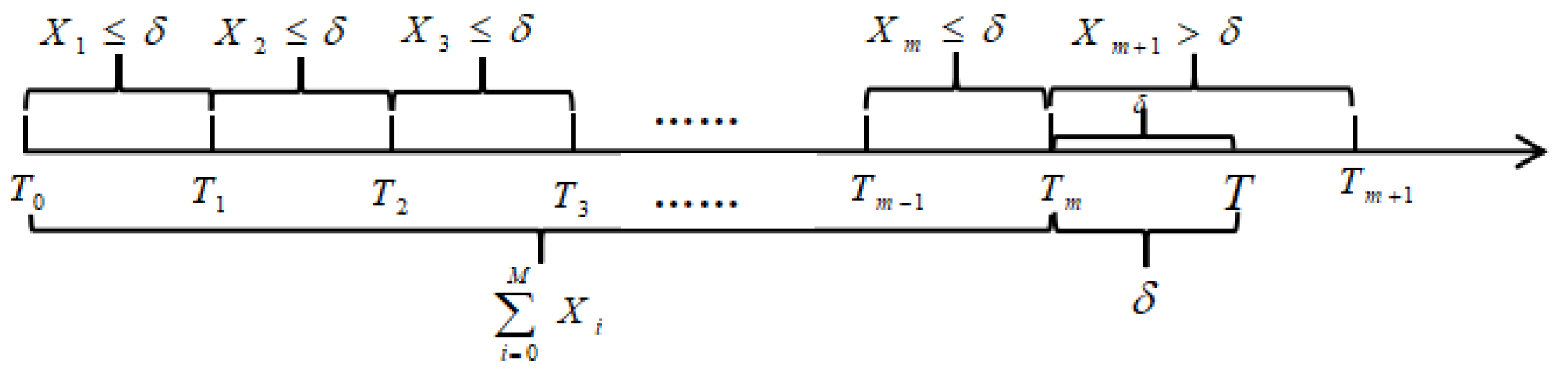
- The system suffers from external shocks. The arrival of the external shocks follows a generalized Pólya process with a set of parameters , , . The system fails when the interval time of successive shocks is larger than . After the nth repair, the system failure threshold decreases as . Denote as the first failure time of the system and let be the operating time of the system after the th repair to the nth failure, where .
- (3)
- Let represent the repair time of the system after the nth failure, where . The repair time sequence forms an increasing geometric process; then, . In particular, when , the maintenance time is ignored.
- (4)
- The system repair cost per unit time is , the operating reward rate per unit time is , the replacement cost is , and the replacement time is negligible.
- (5)
- The GPP, , and are independent.
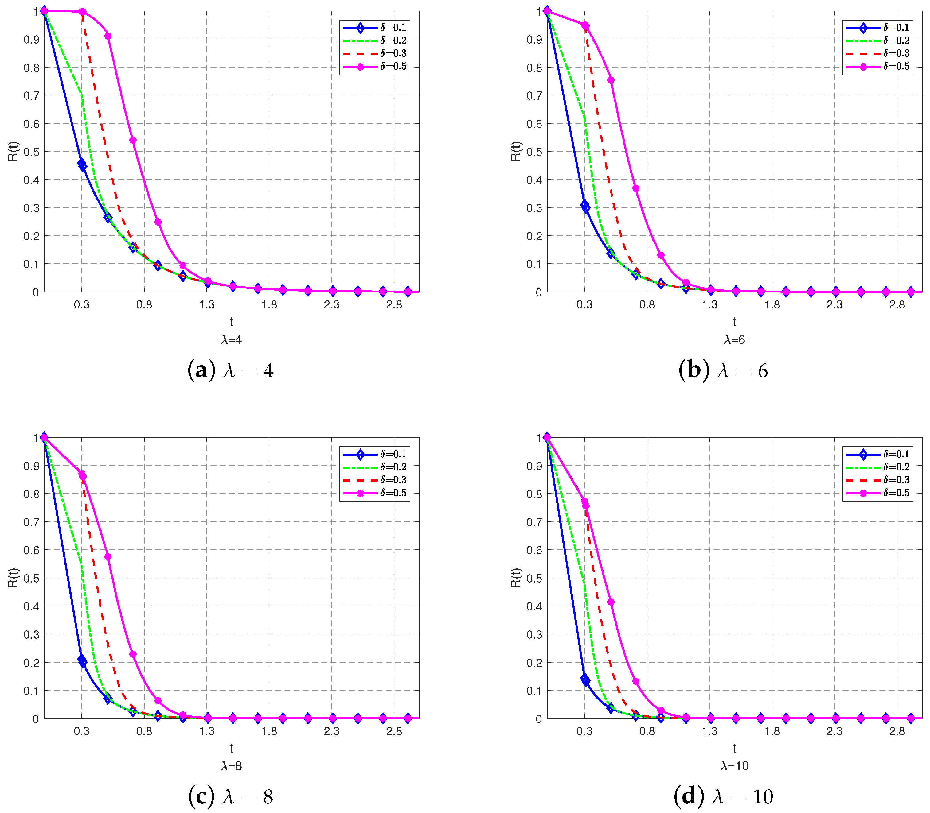
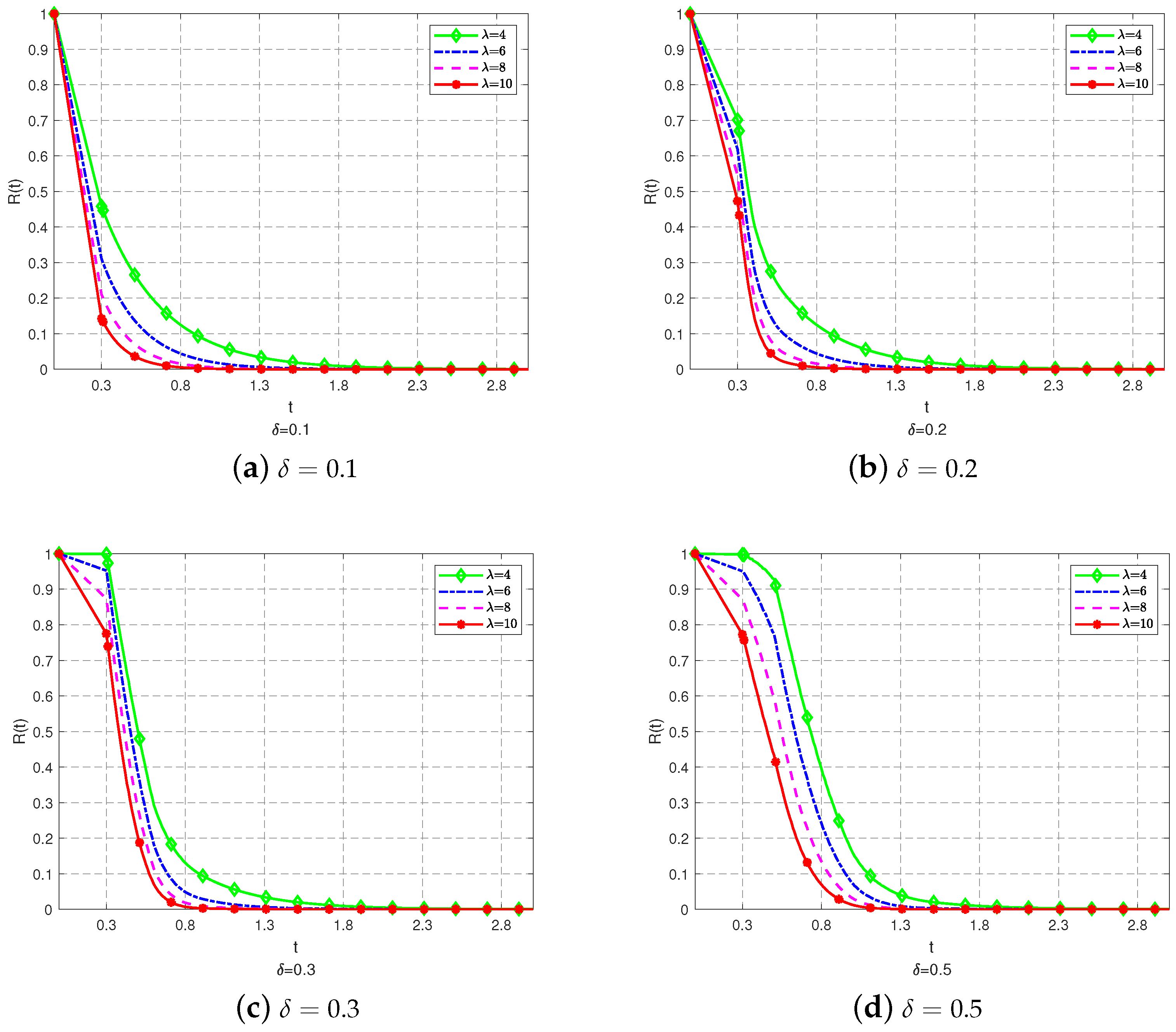
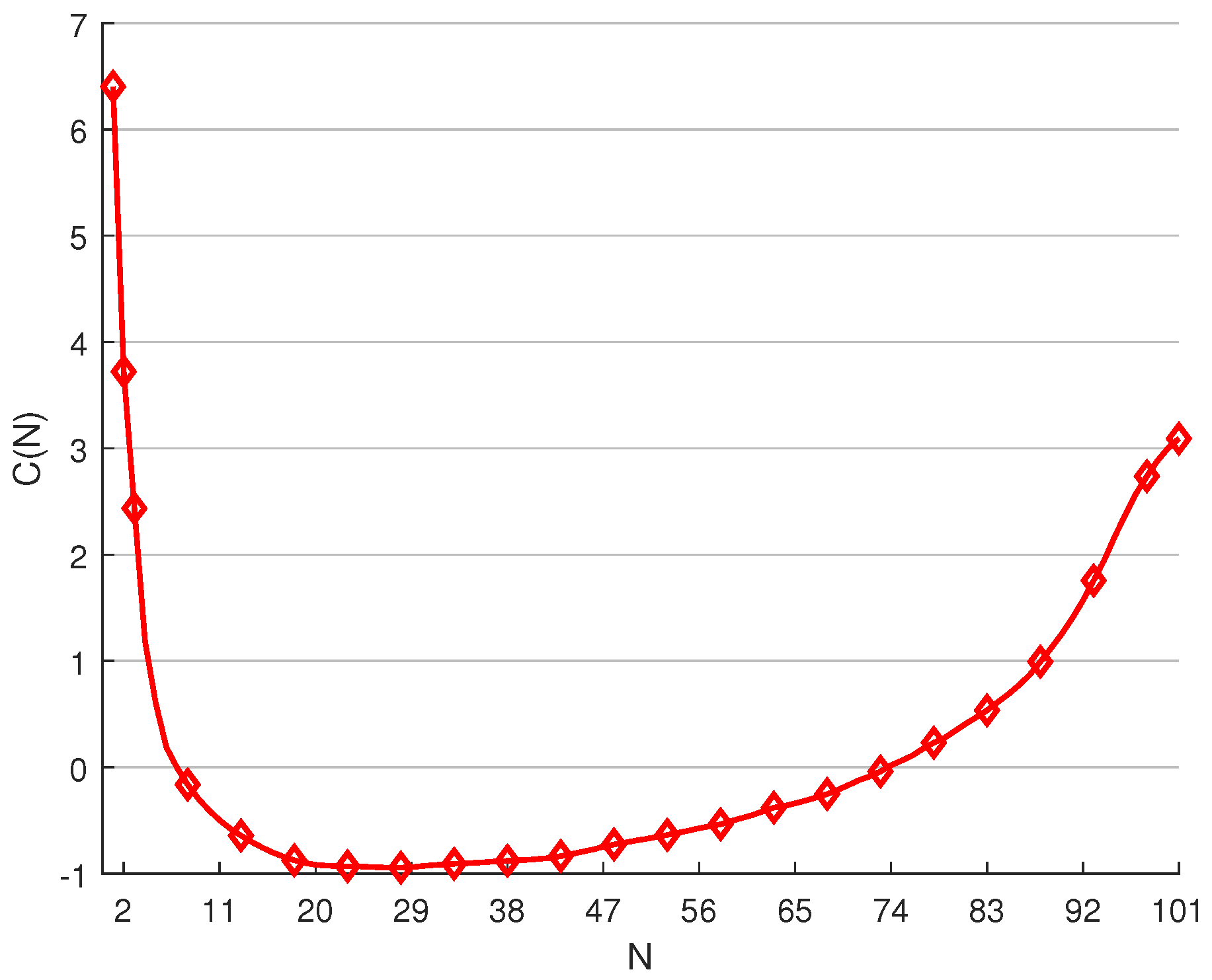
5. Case Study
6. Conclusions
Author Contributions
Funding
Data Availability Statement
Acknowledgments
Conflicts of Interest
Abbreviations
| Notations | |
| T | Life of the system |
| Total shocks number occurred by time t | |
| Stochastic intensity of the generalized Pólya process | |
| Intensity function, | |
| Parameters of the generalized Pólya process | |
| The arrival of external shocks | |
| M | The number of shocks until the system fails |
| The inter-arrival time between the ith and the th shocks | |
| The failure threshold of the censored shock model | |
| The failure rate of the system | |
| The density function of system lifetime T | |
| The distribution function of system lifetime T | |
| The reliability function of system lifetime T | |
| The mean lifetime of the system | |
| J | The Jacobian determinant |
| The conditional density function of | |
| The repair time of the system after the nth failure, | |
| System repair cost per unit time | |
| Operating reward rate per unit time | |
| Replacement cost | |
| N | Replacement policy |
| W | Random length of a cycle under the replacement policy N |
| Expected length of the renewal cycle | |
| Long-run average cost per time | |
| m | The real value of |
| , | Parameters of the generalized Pólya process |
| Acronym | |
| Customer relationship management | |
| Customer lifetime value | |
| Generalized Pólya process | |
| Homogeneous Poisson process | |
| Non-homogeneous Poisson process | |
| Increasing failure rate average | |
| Decreasing failure rate average | |
| Censored shock model | |
| Generalized Pólya censored shock model | |
| Homogeneous Poisson censored shock model | |
| Non-homogeneous Poisson censored shock model |
Appendix A. Proof of Theorem 1
Appendix B. Proof of Theorem 2
Appendix C. Proof of Theorem 4
Appendix D. Proof of Theorem 5
- (1)
- When , i.e., , is increasing, such that ;
- (2)
- When , i.e., , is decreasing, such that .
References
- Esary, J.; Marshall, A. Shock models and wear processes. Ann. Probab. 1973, 1, 627–649. [Google Scholar] [CrossRef]
- Anderson, K. A note on cumulative shock models. J. Appl. Probab. 1988, 25, 220–223. [Google Scholar] [CrossRef]
- Gut, A.; Hüsler, J. Extreme shock models. Extremes 1999, 2, 295–307. [Google Scholar] [CrossRef]
- Mallor, F.; Omey, E. Shocks, runs and random sums. J. Appl. Probab. 2001, 38, 438–448. [Google Scholar] [CrossRef]
- Shanthikumar, J.; Sumita, U. General shock models associated with correlated renewal sequences. J. Appl. Probab. 1983, 20, 600–614. [Google Scholar] [CrossRef]
- Bian, L.; Wang, G.; Liu, P. Reliability analysis for multi-components systems with interdependent competing failure processes. Appl. Math. Model. 2021, 94, 446–459. [Google Scholar] [CrossRef]
- Chen, J.; Li, Z. An extended extreme shock maintenance model for a deteriorating system. Reliab. Eng. Syst. Saf. 2008, 93, 1123–1129. [Google Scholar] [CrossRef]
- Bian, L.; Wang, G.; Duan, F. Reliability analysis for systems subject to mutually dependent degradation and shock processes. Proc. Inst. Mech. Eng. Part J. Risk Reliab. 2021, 235, 1009–1025. [Google Scholar] [CrossRef]
- Li, Z. Some distributions related to Poisson processes and their application in solving the problem of traffic jam. J. Lanzhou Univ. Natural Sci. 1984, 20, 127–136. [Google Scholar]
- Wang, G.; Zhang, Y. A shock model with two-type failures and optimal replacement policy. Int. J. Syst. Sci. 2005, 36, 209–214. [Google Scholar] [CrossRef]
- Eryılmaz, S. Generalized δ-shock model via runs. Stat. Probab. Lett. 2012, 82, 326–331. [Google Scholar] [CrossRef]
- Bian, L.; Wang, G.; Liu, P.; Duan, F. Two shock models for single-component systems subject to mutually dependent failure processes. Qual. Reliab. Eng. Int. 2022, 38, 635–658. [Google Scholar] [CrossRef]
- Wang, G.; Peng, R. A generalised δ-shock model with two types of shocks. Int. J. Syst. Sci. Oper. Logist. 2017, 4, 372–383. [Google Scholar] [CrossRef]
- Wang, G.; Yam, R. Generalized geometric process and its application in maintenance problems. Appl. Math. Model. 2017, 49, 554–567. [Google Scholar] [CrossRef]
- Wang, G.; Zhang, Y.; Yam, R. Preventive maintenance models based on the generalized geometric process. IEEE Trans. Reliab. 2017, 66, 1380–1388. [Google Scholar] [CrossRef]
- Lyu, H.; Ma, L.; Qu, H.; Yang, Z.; Jiang, Y.; Lu, B. Reliability modeling of dependent competing failure processes based on time-dependent threshold level δ and degradation rate changes. Qual. Reliab. Eng. Int. 2023, 39, 2295–2310. [Google Scholar] [CrossRef]
- Ma, M.; Li, Z. Life behavior of censored δ-shock model. Indian J. Pure Appl. Math. 2010, 41, 401–420. [Google Scholar] [CrossRef]
- Eryilmaz, S.; Bayramoglu, K. Life behavior of δ-shock models for uniformly distributed interarrival times. Stat. Pap. 2014, 55, 841–852. [Google Scholar] [CrossRef]
- Bai, J.; Ma, M.; Yang, Y. Parameter estimation of the censored δ-shock model on uniform interval. Commun. Stat.-Theory Methods 2017, 46, 6936–6946. [Google Scholar]
- Bian, L.; Ma, M.; Liu, H.; Ye, J. Lifetime distribution of two discrete censored δ shock models. Commun. Stat.-Theory Methods 2019, 48, 3451–3463. [Google Scholar] [CrossRef]
- Ma, M.; Bian, L.; Liu, H.; Ye, J. Lifetime behavior of discrete Markov chain censored δ shock model. Commun. Stat.-Theory Methods 2021, 50, 1019–1035. [Google Scholar] [CrossRef]
- Ma, M.; Shi, A.; Wang, M. Reliability of Poisson censored δ-shock model. Commun. Stat.-Theory Methods 2022, 52, 8501–8514. [Google Scholar] [CrossRef]
- Chadjiconstantinidis, S.; Eryilmaz, S. Reliability assessment for censored δ-shock Models. Methodol. Comput. Appl. Probab. 2022, 24, 3141–3173. [Google Scholar] [CrossRef]
- Ross, S. Stochastic Processes; John Wiley & Sons: Hoboken, NJ, USA, 1995. [Google Scholar]
- Teugels, J.; Vynckier, P. The structure distribution in a mixed Poisson process. J. Appl. Math. Stoch. Anal. 1996, 9, 489–496. [Google Scholar] [CrossRef]
- Albrecht, P. On some statistical methods connected with the mixed Poisson process. Scand. Actuar. J. 1982, 1, 1–14. [Google Scholar] [CrossRef]
- Eryilmaz, S. δ-shock model based on Polya process and its optimal replacement policy. Eur. J. Oper. Res. 2017, 263, 690–697. [Google Scholar] [CrossRef]
- Konno, H. On the exact solution of a generalized Pólya process. Adv. Math. Phys. 2010, 504267, 1–12. [Google Scholar] [CrossRef]
- Cha, J. Characterization of the generalized Pólya process and its applications. Adv. Appl. Probab. 2014, 46, 1148–1171. [Google Scholar] [CrossRef]
- Cha, J.; Finkelstein, M. New shock models based on the generalized Pólya process. Eur. J. Oper. Res. 2016, 251, 135–141. [Google Scholar] [CrossRef]
- Goyal, D.; Finkelstein, M.; Hazra, N. On history-dependent mixed shock models. Probab. Eng. Informational Sci. 2021, 36, 1080–1097. [Google Scholar] [CrossRef]
- Goyal, D.; Hazra, N.; Finkelstein, M. On the time-dependent delta-shock model governed by the generalized Pólya process. Methodol. Comput. Appl. Probab. 2022, 24, 1627–1650. [Google Scholar] [CrossRef]
- Goyal, D.; Hazra, N.; Finkelstein, M. On the general δ-shock model. Methodol. Comput. Appl. Probab. 2022, 31, 994–1029. [Google Scholar] [CrossRef]
- Barlow, R.; Proschan, F. Statistical Theory of Reliability and Life Testing: Probability Models; Holt, Rinehart and Winston: New York, NY, USA, 1975. [Google Scholar]

| Model | Parameter | Failure Mechanism | System Lifetime |
|---|---|---|---|
| shock model | |||
| censored shock model |
| N | N | N | N | N | |||||
|---|---|---|---|---|---|---|---|---|---|
| 1 | 13 | 30 | 54 | 78 | 0.1974 | ||||
| 2 | 14 | 32 | 56 | 80 | 0.3798 | ||||
| 3 | 15 | 34 | 58 | 82 | 0.5038 | ||||
| 4 | 16 | 36 | 60 | 84 | 0.5941 | ||||
| 5 | 17 | 38 | 62 | 86 | 0.7549 | ||||
| 6 | 18 | 40 | 64 | 88 | 1.2810 | ||||
| 7 | 20 | 42 | 66 | 90 | 1.3709 | ||||
| 8 | 22 | 44 | 68 | 92 | 1.6431 | ||||
| 9 | 24 | 46 | 70 | 0.1368 | 94 | 2.0699 | |||
| 10 | 26 | 48 | 72 | 0.1567 | 96 | 2.4149 | |||
| 11 | 28 | 50 | 74 | 0.1693 | 98 | 2.5950 | |||
| 12 | 29 | −0.9944 | 52 | 76 | 0.1859 | 100 | 3.0909 |
Disclaimer/Publisher’s Note: The statements, opinions and data contained in all publications are solely those of the individual author(s) and contributor(s) and not of MDPI and/or the editor(s). MDPI and/or the editor(s) disclaim responsibility for any injury to people or property resulting from any ideas, methods, instructions or products referred to in the content. |
© 2023 by the authors. Licensee MDPI, Basel, Switzerland. This article is an open access article distributed under the terms and conditions of the Creative Commons Attribution (CC BY) license (https://creativecommons.org/licenses/by/4.0/).
Share and Cite
Bian, L.; Peng, B.; Ye, Y. Reliability Analysis and Optimal Replacement Policy for Systems with Generalized Pólya Censored δ Shock Model. Mathematics 2023, 11, 4560. https://doi.org/10.3390/math11214560
Bian L, Peng B, Ye Y. Reliability Analysis and Optimal Replacement Policy for Systems with Generalized Pólya Censored δ Shock Model. Mathematics. 2023; 11(21):4560. https://doi.org/10.3390/math11214560
Chicago/Turabian StyleBian, Lina, Bo Peng, and Yong Ye. 2023. "Reliability Analysis and Optimal Replacement Policy for Systems with Generalized Pólya Censored δ Shock Model" Mathematics 11, no. 21: 4560. https://doi.org/10.3390/math11214560
APA StyleBian, L., Peng, B., & Ye, Y. (2023). Reliability Analysis and Optimal Replacement Policy for Systems with Generalized Pólya Censored δ Shock Model. Mathematics, 11(21), 4560. https://doi.org/10.3390/math11214560