Reliability of Partitioning Metric Space Data

Abstract

The process of sorting or categorizing objects or information about these objects into clusters according to certain criteria is a fundamental procedure in data analysis. Where it is feasible to determine the distance metric for any pair of objects, the significance and reliability of the separation can be evaluated by calculating the separation/segregation power (SP) index proposed herein. The latter index is the ratio of the average inter distance to the average intra distance, independent of the scale parameter. Here, the calculated SP value is compared to its statistical distribution obtained by a simulation study for a given partition under the homogeneity null hypothesis to draw a conclusion using standard statistical procedures. The proposed concept is illustrated using three examples representing different types of objects under study. Some general considerations are given regarding the nature of the SP distribution under the null hypothesis and its dependence on the number of divisions and the amount of data within them. A detailed modus operandi (working method) for analyzing a metric data partition is also offered.

1. Introduction

Attempting to understand, take control of, or resolve a particular quality or reliability problem, initially we often try to classify the objects under study (OUS) into relatively homogeneous groups. For example, when analyzing the problem of accumulating a large inventory of faulty products of a certain type, we will likely try to divide them into groups provided by different suppliers and, if such a division makes sense, we will use methods that will force these suppliers to compete to supply higher quality products in the hope of being the supplier of choice—divide et impera!

In recent decades, new types of quality and reliability data have been appearing at a pace that sometimes exceeds our ability to comprehend and interpret them [1,2,3,4,5]. The partition of data arrays into clusters, in accordance with some criterion, is a necessary step in the study of a particular phenomenon. The subsequent investigation must confirm or refute the expediency of such a division. If confirmed, the criterion’s discriminatory power must be assessed (or, in other words, the influencing power of a factor in accordance with the levels of which the data were partitioned must be evaluated). If the data come from a metric space, then for any pair of data, a distance characterizing the dissimilarity between them is defined. Choosing the appropriate distance metric is a fundamental problem in quality control, pattern recognition, machine learning, cluster analysis, etc.

Data do not necessarily mean numbers; data can be information of any kind about the OUS, obtained as a result of tests, measurements, observations, inquiries, etc. The distance between data, however, indicating how far apart the studied objects are (i.e., dissimilar), is represented by a scalar/number. Notwithstanding all the shortcomings of such a simplification of the representation of the distinction between complex objects, this idea has one undeniable advantage: simplicity.

In metric space, distance d satisfies the following four axioms:

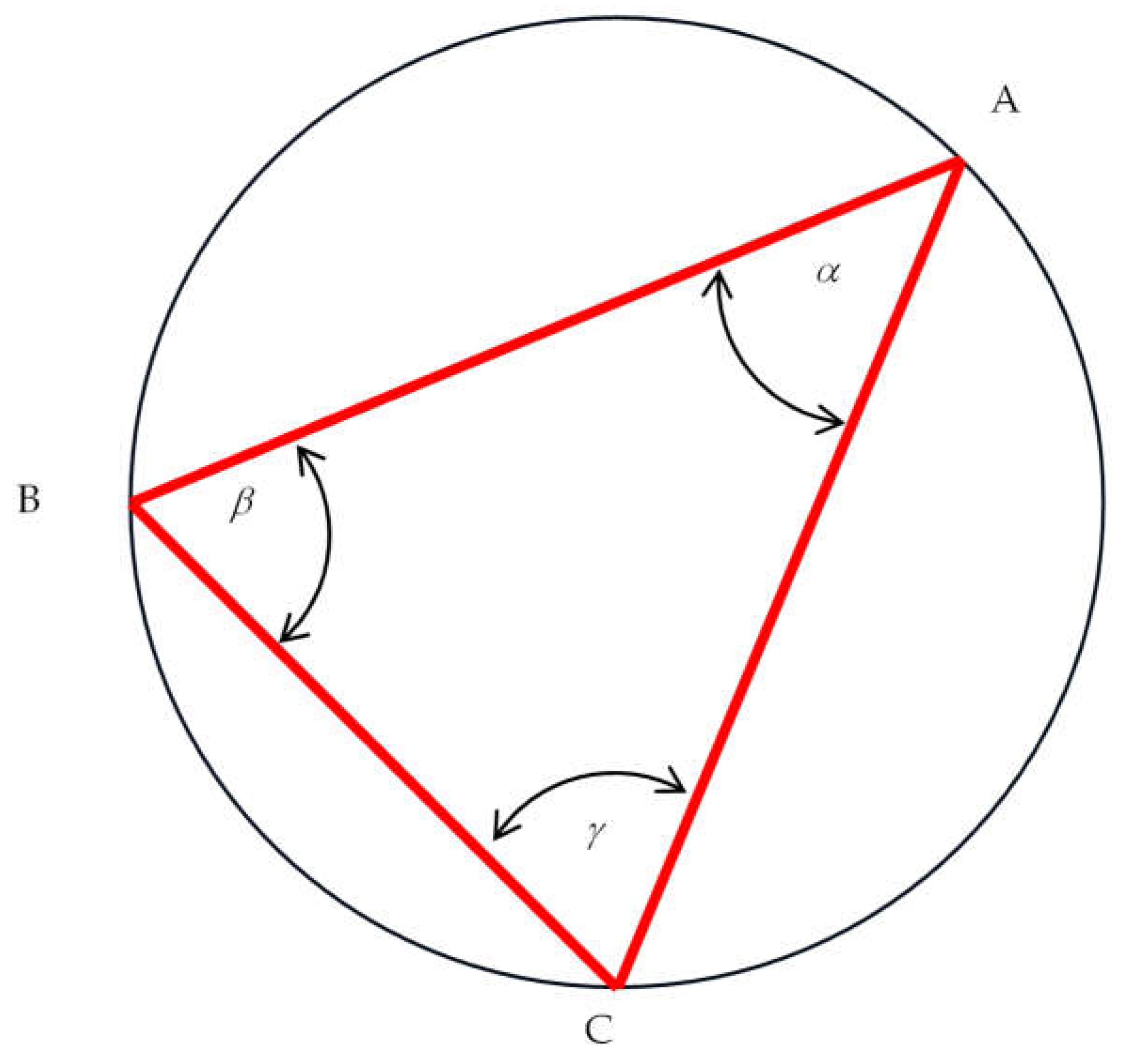
• The distance from a data point to itself is zero: d(x, x) = 0.
• The distance between two distinct points x and y is always positive: d(x, y) > 0.
• The distance from x to y is always the same as the distance from y to x: d(x, y) = d(y, x).
• There is a triangle inequality: d(x, y) + d(y, z) ≤ d(x, z).

The OUS, as well as the data characterizing them, can be very diverse. In our recent article [1], we considered some new types of quality data: categorical, preference chains, strings, shapes, images, tree structured, and product/process distributions. In the short time since the paper was published, not surprisingly, more and more data types have emerged. The continually expanding spectrum of distance metrics used in quality and reliability engineering is also diverse (Figure 1); e.g., see [6] for the use of Wasserstein and Hausdorff metrics for quality control and cyber-attack detection.

Here we assume that in accordance with a selected metric, for a data set ${\left\{X_i\right\}}_{i=1}^N$, of size $N$, related to the phenomenon under study, a matrix d_ij = d(x_i, x_j) of mutual distances for each pair of data x_i and x_j can be determined. This is a symmetric square matrix with non-negative entries and zeros on the main diagonal. From the triangle inequality (axiom 4), it follows that d_ik + d_kj ≤ d_ij for any triad of i, j, and k.

To ascertain the influencing factors, all the data are divided into m groups/segments of size $n_1,n_2, \dots ,n_k, \dots ,n_m$ $(\sum _{k=1}^m{n}_k=N)$ according to a criterion associated with the levels of this/these factor/factors. Respectively, all $\left(\begin{array}{c}N\\ 2\end{array}\right)$ distances are split into two types (Figure 2): those that refer to data pairs belonging to the same group (denoted here by the prefix intra) and those that describe the distances between pairs of data belonging to different groups (denoted here by the prefix inter).

To ascertain whether this partitioning is effective and, if so, to what extent, the degree of distinction achieved, henceforth called segregation power—SP [7]—must be evaluated. If the discrimination turns out to be weak (statistically insignificant), the hypothesis that the partitioning criterion was chosen incorrectly could be accepted. If, on the other hand, the discrimination is not weak (statistically significant), this evaluation should be compared to other partitioning criteria. This article is devoted to the development of a measure suitable for this purpose. The attentive reader will certainly find some analogies with ANOVA; however, the proposed approach differs both in general and in specific details from the latter.

2. Preliminary Materials: Some Definitions and Separation Power (SP) Calculation Method

Before explaining our method, we define some of the concepts used herein.

2.1. Some Definitions

• Intra degrees of connection ${dc}_{intra}$: The sum of data pairs belonging to the same groups, i.e.,
• ${dc}_{intra}=\sum _{i=1}^m\left(\begin{array}{c}{n}_i\\ 2\end{array}\right)=\left(\begin{array}{c}{n}_1\\ 2\end{array}\right)+\left(\begin{array}{c}{n}_2\\ 2\end{array}\right)+\dots .+\left(\begin{array}{c}{n}_m\\ 2\end{array}\right).$
• Inter degrees of connection ${dc}_{inter}$: The sum of data pairs belonging to the different groups, i.e.,
• ${dc}_{inter}=\sum _{i=1}^m\sum _{j>1}^m{n}_i{n}_j=\frac{1}{2}\sum _{i\ne j}{n}_i{n}_j$.
• Total degrees of connection ${dc}_{total}$: The sum of all data pairs, i.e.,
• $d{c}_{total}=\left(\begin{array}{c}N\\ 2\end{array}\right)$. Obviously,
• $d{c}_{total}=d{c}_{intra}+d{c}_{total}=d{c}_{inter}$.
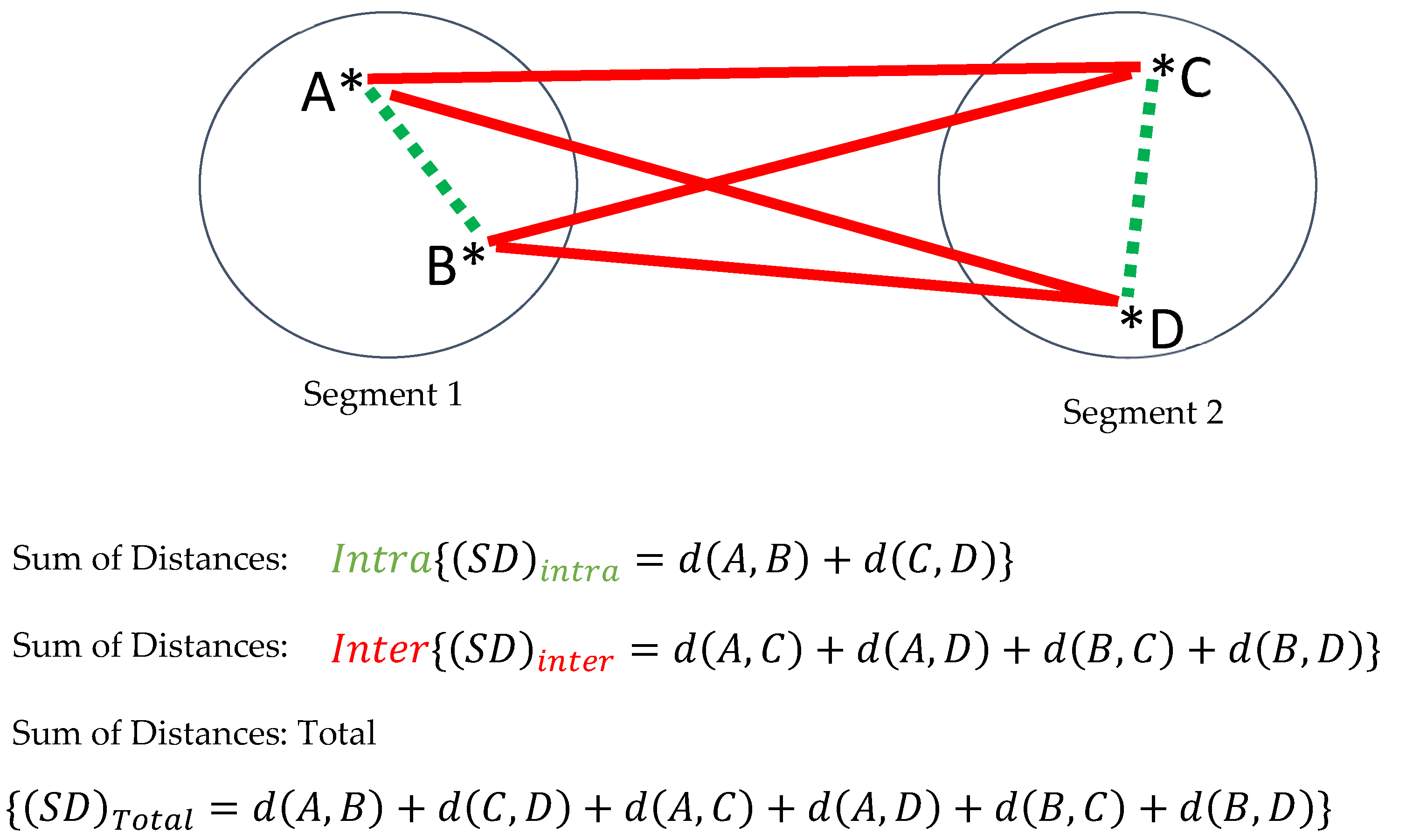
• Intra sum of distances ${SD}_{intra}$: The sum of distances between data pairs belonging to the same groups.
• Inter sum of distances ${SD}_{inter}$: The sum of distances between data pairs belonging to the different groups.
• Total sum of distances ${SD}_{total}$: The sum of distances between all data pairs. Obviously (see Figure 3 for an example),
• ${SD}_{total}={SD}_{intra}+{SD}_{inter}$.
• Intra mean distance ${MD}_{intra}$: The sum of distances between data pairs belonging to the same groups ${SD}_{intra}$ divided by the intra degrees of connection—${dc}_{intra}$—i.e., ${MD}_{intra}=\frac{{SD}_{intra}}{{dc}_{intra}}$;
• Inter mean distance ${MD}_{inter}$: The sum of distances between data pairs belonging to the different groups ${SD}_{inter}$ divided by the inter degrees of connection—${dc}_{inter}$—i.e., ${MD}_{inter}=\frac{{SD}_{inter}}{{dc}_{inter}}$.
• Separation/segregation power—SP$: {MD}_{inter}$ divided by ${MD}_{intra}$, i.e.,

$$SP=\frac{M{D}_{inter}}{M{D}_{intra}}=\frac{S{D}_{inter}/{dc}_{inter}}{S{D}_{intra}/{dc}_{intra}}$$

(1)

2.2. Some Illustrative Examples of SP Calculation for the Different Kinds of Data

We start with the simplest example and continue with more complex ones.

2.2.1. Data Represented by Real Numbers

Times to failure (TTFs) of two products (A and B) randomly selected from the batch supplied by supplier I were 24,000 and 30,000 h, respectively, while the TTFs of two other products (C and D) randomly selected from the batch supplied by supplier II were 17,000 and 19,000 h, respectively. In other words, X_A = 24,000 and X_B = 30,000, whereas X_C = 17,000 and X_D = 19,000. Given this information, let us divide these data into two groups as in Figure 3. The first is A, B (supplier I), and the second is C, D (supplier II). Choosing the range between the TTFs as the distance measure (Euclidean distance), we obtain the matrix of mutual distances shown in

Table 1. The matrix of mutual distances between TTFs.

	A	B	C	D
A	0	6000	7000	5000
B	6000	0	13,000	11,000
C	7000	13,000	0	2000
D	5000	11,000	2000	0

.

Hence, in line with definitions provided above and in Figure 3:

$$S{D}_{intra}=d_{A,B}+d_{C,D}=6000+2000=8000$$

$$d{c}_{intra}=2$$

$$S{D}_{inter}=d_{A,C}+d_{A,D}+d_{B,C}+d_{B,D}=7000+5000+13000+11000=36000$$

$$d{c}_{inter}=4$$

Accordingly,

$$M{D}_{intra}=\frac{8000}{2}=4000; M{D}_{inter}=\frac{36000}{4}=9000$$

and finally:

$$SP=\frac{M{D}_{inter}}{M{D}_{intra}}=\frac{9000}{4000}=2.25$$

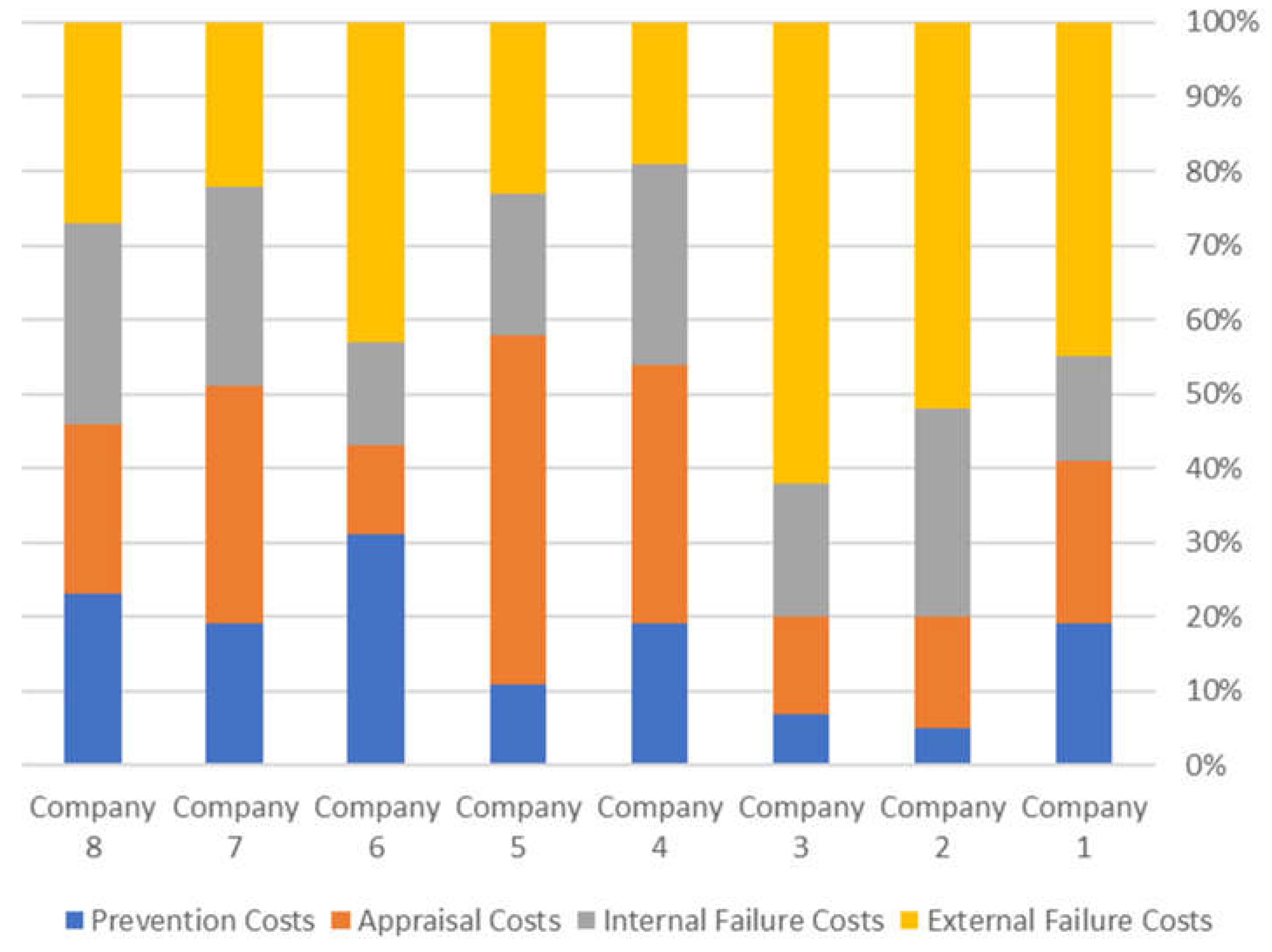
2.2.2. Each Datum Is a Discrete Distribution over Categories (as in a Pie Chart)

Below are real data on the distribution of quality cost proportions by four categories defined by [8] for eight Israeli companies engaged in residential construction in Israel [9] (see

Table 2. Distribution of proportions of quality costs in four categories ([9], p. 109).

	Company 1	Company 2	Company 3	Company 4	Company 5	Company 6	Company 7	Company 8
Prevention costs	0.19	0.05	0.07	0.19	0.11	0.31	0.19	0.23
Appraisal costs	0.22	0.15	0.13	0.35	0.47	0.12	0.32	0.23
Internal failure costs	0.14	0.28	0.18	0.27	0.19	0.14	0.27	0.27
External failure costs	0.45	0.52	0.62	0.19	0.23	0.43	0.22	0.27
Total	1	1	1	1	1	1	1	1

and Figure 4). Although all surveyed companies were certified to the international quality standard, it was striking that companies 1, 2, 3, and 6 spent relatively much more on external failures than the other companies (4, 5, 7, and 8). Let us now calculate the SP between these two clusters. Four proportions reflecting the distribution of quality costs across the whole spectrum of possible costs are known for each company.

The most appropriate distance measure for comparing two distributions ($p_1,\dots p_i,\dots ,p_r$) and ($q_1,\dots q_i,\dots ,q_r$) on a nominal scale is the Hellinger distance, defined as [10]:

$$H\left(P,Q\right)=\frac{1}{\sqrt{2}}\sqrt{\sum _{i-1}^r{\left(\sqrt{p_i}-\sqrt{q_i}\right)}^2}$$

In our case, because we have four quality cost categories, r = 4. Using this distance measure, we obtain the matrix of mutual distances shown in

Table 3. Matrix of mutual distances between companies.

	Company 1	Company 2	Company 3	Company 4	Company 5	Company 6	Company 7	Company 8
Company 1	0.000	0.198	0.169	0.214	0.222	0.122	0.189	0.152
Company 2	0.198	0.000	0.094	0.290	0.290	0.265	0.265	0.240
Company 3	0.169	0.094	0.000	0.328	0.320	0.230	0.302	0.266
Company 4	0.214	0.290	0.328	0.000	0.120	0.269	0.030	0.104
Company 5	0.222	0.290	0.320	0.120	0.000	0.317	0.127	0.191
Company 6	0.122	0.265	0.230	0.269	0.317	0.000	0.244	0.178
Company 7	0.189	0.265	0.302	0.030	0.127	0.244	0.000	0.077
Company 8	0.152	0.240	0.266	0.104	0.191	0.178	0.077	0.000

.

The total degrees of connection are dc_total = 28 (“two out of eight” combinations) split into dc_intra = 12 (twice “two out of four”) and dc_inter = 16 (combinations of each of the four proportions in the first cluster with each of the four proportions in the second cluster). Skipping the routine of calculating the sums of the intra and inter distances, in

Table 4. The total degree of connection split.

$S{D}_{intra}=1.727$	${dc}_{intra}=12$	$M{D}_{intra}=\frac{S{D}_{intra}}{{dc}_{intra}}=0.144$
$S{D}_{inter}=4.082$	${dc}_{inter}=16$	$M{D}_{inter}=\frac{S{D}_{inter}}{{dc}_{inter}}=0.255$
$S{D}_{total}=5.809$	${dc}_{total}=28$

we present only the results.

And finally, $SP=\frac{M{D}_{inter}}{M{D}_{intra}}=1.773$.

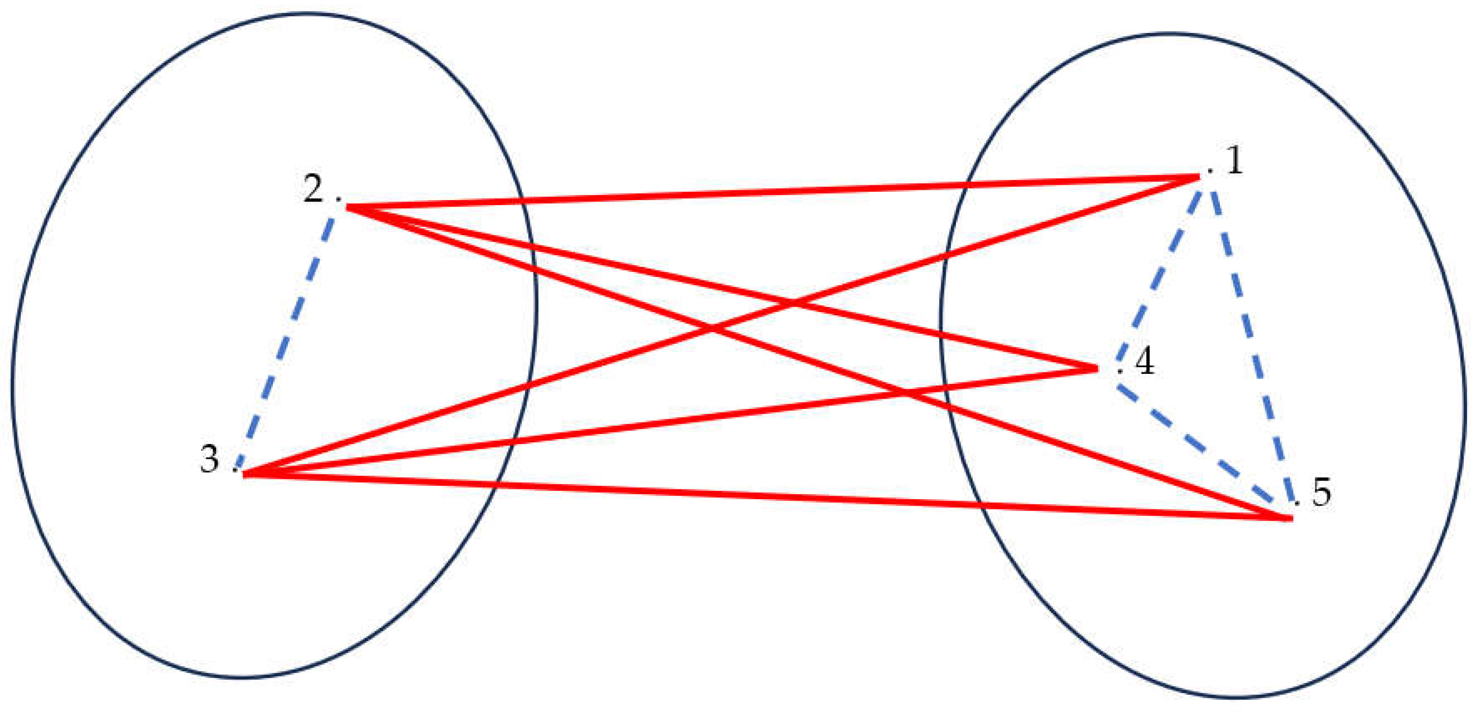
2.2.3. Each Datum Is a Preference Chain of Alternatives

Preference/prioritization chains (PC), along with other new types of structured data, are widely used in engineering, quality management, risk management, genetics, healthcare, customer research, decision making, etc. Let the symbol “>” depict the relationships between two alternatives, i.e., A₁ > A₂ means that A₁ is preferable to A₂. A set of n predetermined alternatives arranged as a string by this symbol (e.g., A₁ > A₂ > A₃> … > A_n) forms a strict preference chain. Obviously, there are n! such chains obtained by permutation of the alternatives. The construction of a chain is based only on relationships among the predetermined alternatives without necessarily being related to the evaluation of the property under study.

According to [11,12], all feasible PCs are scattered on the surface of the n(n − 1)/2-dimensional sphere. If one of them—for example, the naturally ordered chain A₁ > A₂ > A₃ > … > A_n—is considered as a base, the north pole ([N]), then the reverse chain is located on the south pole [S] of this sphere and all the remaining (n! − 2) PCs are located on [n(n − 1)/2] − 1 parallels formed by flat disks, which cut the N–S axis equidistantly. The so-called geodesic distance between two PCs is proportional to the length of the geodesic arc connecting them on the surface of a multidimensional globe. The radius of this globe, for convenience, is chosen so that the maximum possible distance (e.g., from [N] to [S]) is equal to 1. For details regarding calculation of the geodetic distance, we refer readers to [11].

In one of the experiments described in [11], five experts/judges prioritize five alternatives. Judges two and three are women, while judges one, four, and five are men.

Table 5. Distance matrix between each pair of judges.

		Judge j
		1	2	3	4	5
Judge i	1	0	0.59	0.73	0.33	0.38
	2	0.59	0	0.46	0.45	0.44
	3	0.73	0.46	0	0.65	0.61
	4	0.33	0.45	0.65	0	0.37
	5	0.38	0.44	0.61	0.37	0

shows the mutual distances between the respective preference chains.

To check the discrimination power of gender (if such exists), we divide the five judges into two clusters (2, 3) and (1, 4, 5) according to gender; see Figure 5.

Then,

• $M{D}_{intra}=\frac{\left[d_{\mathrm{2,3}}+\left(d_{\mathrm{1,4}}+d_{\mathrm{1,5}}+d_{\mathrm{4,5}}\right)\right]}{4}=0.385$
• $M{D}_{inter}=\frac{\left[(d_{\mathrm{2,1}}+d_{\mathrm{2,4}}+d_{\mathrm{2,5}})+\left(d_{\mathrm{3,1}}+d_{\mathrm{3,4}}+d_{\mathrm{3,5}}\right)\right]}{6}=0.578$

This implies $SP=\frac{M{D}_{inter}}{M{D}_{intra}}=1.502$.

2.3. Checking the Homogeneity Hypothesis H₀

In its most general form, the conservative (null) hypothesis of homogeneity H₀ means that data being studied across all groups are drawn from the same initial original population distribution. In other words, the scatter of data, of course, reflects the scatter of data within the population itself, but in no way indicates the influence of the level of the factor, in accordance with which the partitioning into groups was made, on the data being studied. Thus, the division of data into groups/segments does not make any sense, and the difference in the data is due to noise factors only. For example, when analyzing the academic achievements of students, an assumption H₀ can mean the independence of the latter from a characteristic/factor such as gender or hair color.

As in ANOVA, we assume that if SP exceeds a certain threshold, determined for a given risk by the distribution of the SP under H₀, it can serve as an indicator of the influence of a discriminating/segregating factor. The p-value can also serve as an indicator of discrimination/segregation: the smaller it is, the greater the influence of the segregating factor. The considerations given in Section 3.1 and Appendix A, Appendix B and Appendix C support the proposition that, for a given H₀, the distribution of SP depends only on the type of partition, i.e., vector ($n_1,n_2,\dots ,n_k,\dots ,n_m)$. Some general conclusions about the SP distribution can be made on the basis of an analytical analysis supported by simulation (see Section 3 and Appendix A, Appendix B and Appendix C).

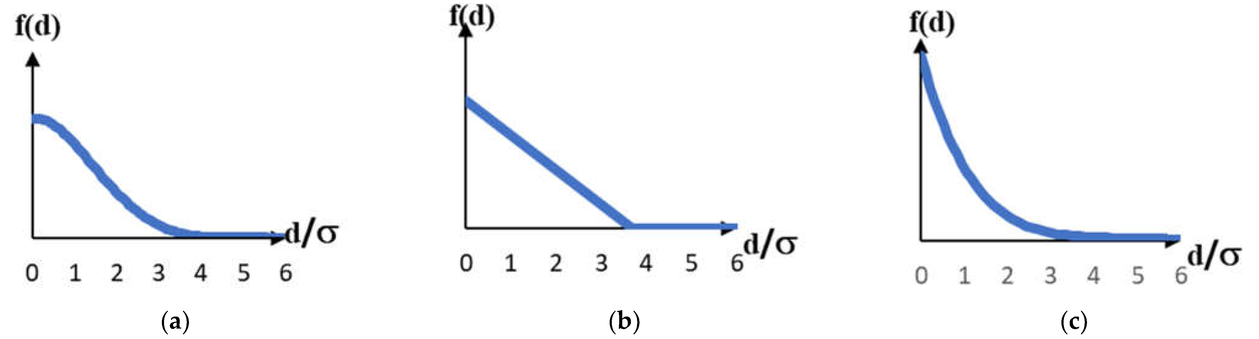
2.4. Some Simple Examples of Distance Metric Distribution

Suppose we have a pair of data points randomly and independently drawn from the same distribution and the distance d is defined as a range between them.

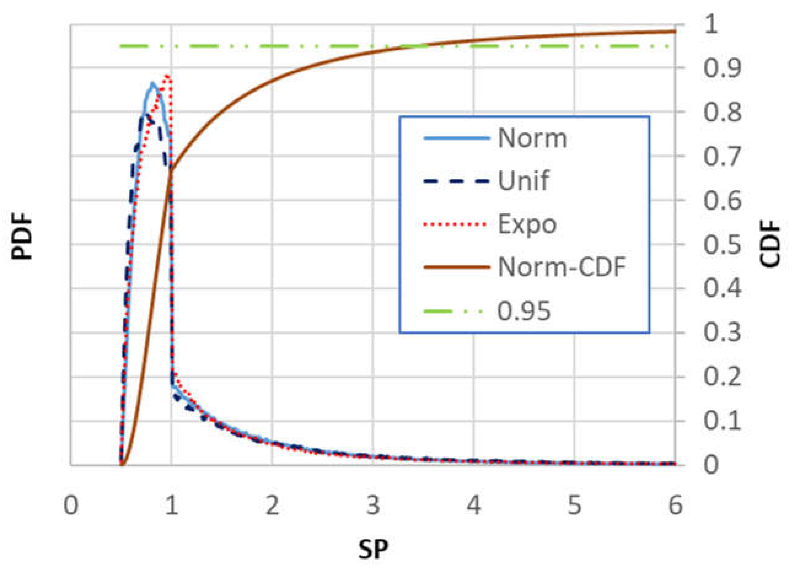
2.4.1. Normal Distribution

If the distribution is normal, then d is distributed according to (2a) (see Figure 6a [13,14]):

$$f\left(d\right)=\frac{1}{\sigma \sqrt{\pi }}{e}^{-{\left(\frac{d}{2\sigma }\right)}^2} (d\ge 0),$$

(2a)

where σ is the standard deviation of the original normal distribution $N\left(\mu ,{\sigma }^2\right)$ and f(d) means the probability density function (PDF).

Clearly, the mean distance as well as its variance depend on the scale parameter σ of the native normal distribution only:

$$E\left(d\right)=\frac{2}{\sqrt{\pi }}\sigma$$

(3a)

$$VAR\left(d\right)=\left(2-\frac{4}{\pi }\right){\sigma }^2$$

(4a)

2.4.2. Uniform Distribution

Now suppose a pair of data points are randomly and independently drawn from the same uniform distribution U(a, b); then the distance d between them is distributed according to the triangular distribution (2b) (see Figure 6b [15,16]):

$$f\left(d\right)=\frac{2}{b-a}\left(1-\frac{d}{b-a}\right), (0\le d\le b-a)$$

(2b)

with

$$E\left(d\right)=\frac{2}{\sqrt{3}}\sigma$$

(3b)

$$VAR\left(d\right)=\frac{2}{3}{\sigma }^2$$

(4b)

where ${\sigma }^2=\frac{{\left(b-a\right)}^2}{12}$ denotes the variance of the uniform distribution U(a, b). Both Equations (3b) and (4b) do not depend on the location parameter (a + b)/2 of U(a, b).

2.4.3. Exponential Distribution

Finally, in the case of an exponential distribution $Exp(x_0,\lambda )$, anchored at the “starting” value $x_0$ (location parameter), and the spread reciprocal λ, the distance d is distributed according to Equation (2c) (see Figure 6c [15,16]):

$$f\left(d\right)=\lambda e^{-\lambda d} (d\ge 0)$$

(2c)

with

$$E\left(d\right)=\sigma$$

(3c)

$$VAR\left(d\right)={\sigma }^2$$

(4c)

where $\sigma =\frac{1}{\lambda }$ denotes the standard deviation of the exponential distribution $Exp(x_0,\lambda )$.

2.4.4. Conclusions Derived from the above Examples

Naturally, independence of the pairwise distance distribution on the location parameter of the original native data distribution holds not only for the distributions mentioned above. It holds for any kind of data distribution for which the location and the scale parameters can be determined independently. In this sense, we can talk about the translational invariance of the distance distribution. Consequently, under H₀, both E(SD_intra) and E(SD_inter), given partitioning, do not depend on the location parameter and are proportional to the scale parameter σ. Thus, the ratio E($M{D}_{inter}$)/E($M{D}_{intra}$) does not depend on either the location or the scale parameter, and equals one. The latter gives us a reason to assume that under H₀, the distribution of SP = $M{D}_{inter}/M{D}_{intra}$ also does not depend on these parameters, but is determined only by the method of partitioning and type of original data distribution. Detailed proof of this statement is given in Appendix A and simulation studies provided by the authors for normal, uniform, and exponential original distributions confirm this assumption. Figure 7 illustrates this universal SP distribution for a partition of four data sets as shown in Figure 3. The authors experimented with many different location and scale parameters, and the results were always repeatable. The same thing happened with other types of partitioning, different from those shown in Figure 3 (e.g., A-BCD or more data), used by the authors.

3. Results of the Theoretical and Simulation Studies

3.1. Some General Considerations Regarding SP Distribution under H₀

As noted in Section 2.4.4, expectations of the numerator and denominator of SP under H₀ are equal: E($M{D}_{inter}$) = E($M{D}_{intra}$). Simple conclusions could be drawn regarding the variances of the numerator and denominator of SP, if not for the fact that the terms in both the numerator and the denominator are distributed identically, but not independently; additionally, two distances from a common vertex datum are correlated, not independent (see Appendix B). The specific value of the correlation coefficient ρ (the same for all pairs of correlated distances) depends on the type of original data distribution. In the case of a normal original data distribution, for example, it equals 0.224. It should be noted that correlations exist not only between pairs of distances that are terms in the numerator (or denominator), but also between distances, one of which belongs to the inter connection and the other to the intra connection, if they come from a common vertex datum (e.g., d(A,C) and d(A,B) with common vertex A in Figure 3). It is not difficult to prove that:

$$VAR\left(S{D}_{inter}\right)={dc}_{inter}·VAR\left(d\right)+2·cov·\sum _{i=1}^m\left[n_i·\left(\begin{array}{c}N-n_i\\ 2\end{array}\right)\right]$$

(5)

$$VAR\left(S{D}_{intra}\right)={dc}_{intra}·VAR\left(d\right)+6·cov·\sum _i\left(\begin{array}{c}{n}_i\\ 3\end{array}\right)$$

(6)

$$COV\left(S{D}_{intra},S{D}_{inter}\right)=2·cov·\sum _{i\ne j}\left[n_i·\left(\begin{array}{c}{n}_j\\ 2\end{array}\right)\right]$$

(7)

where VAR(d) means variance of d, e.g., $\left(2-\frac{4}{\pi }\right){\sigma }^2$ for distribution (2a) and $cov$ means covariance between two distances with a common vertex, e.g., $cov=\rho \ast VAR\left(d\right)\approx 0.163{\sigma }^2$ for distribution (2a).

Accordingly,

$$VAR\left(M{D}_{inter}\right)=\frac{VAR\left(d\right)}{d{c}_{inter}}+\frac{2·cov·\sum _{i=1}^m\left[n_i·\left(\begin{array}{c}N-n_i\\ 2\end{array}\right)\right]}{{dc}_{inter}^2}$$

(8)

$$VAR\left(M{D}_{intra}\right)=\frac{VAR\left(d\right)}{d{c}_{intra}}+\frac{6·cov·\sum _{i=1}^m\left(\begin{array}{c}{n}_i\\ 3\end{array}\right)}{{dc}_{intra}^2}$$

(9)

$$COV\left(M{D}_{intra},M{D}_{inter} \right)=\frac{2·cov·\sum _{i\ne j}\left[n_i·\left(\begin{array}{c}{n}_j\\ 2\end{array}\right)\right]}{d{c}_{intra}·d{c}_{inter}}$$

(10)

If there is only a small number of OUS, it is impossible to draw general theoretical conclusions about the shape of the SP distribution under H₀ using Equations (8)–(10) only. In such cases, only multiple simulations under a given partitioning, such as the one discussed in Section 2.4.4, Figure 7, can help. The situation, however, is greatly facilitated when the number of OUS (data) in groups or the number of groups increases (see Appendix C). The more OUS there are, the closer E(SP) is to 1, and the distribution itself narrows. In the limiting case, $E\left(SP\right)\to 1, VAR\left(SP\right)\to 0$. Figure 8a,b illustrate the effect of the number of partition groups m on the cumulative distribution function (CDF) and the PDF of the SP distribution (under H₀, the original data are distributed according to normal distribution, $\forall n=10$). Figure 9 illustrates the effect of the amount of data in every one of ten equally sized groups (m = 2).

3.2. Some Remarks on Deriving the SP Distribution from a Simulation Process under H₀

Since different null hypotheses are possible for different types of OUS, there is no universal SP distribution for a certain partition. Nevertheless, under a certain null hypothesis, such a distribution can be obtained by repeating the data simulation over and over and doing the subsequent SP calculations. The data structure significantly affects the simulation model. This is demonstrated in Section 3.2.1, Section 3.2.2 and Section 3.2.3 using the examples described in Section 2.2.1, Section 2.2.2 and Section 2.2.3.

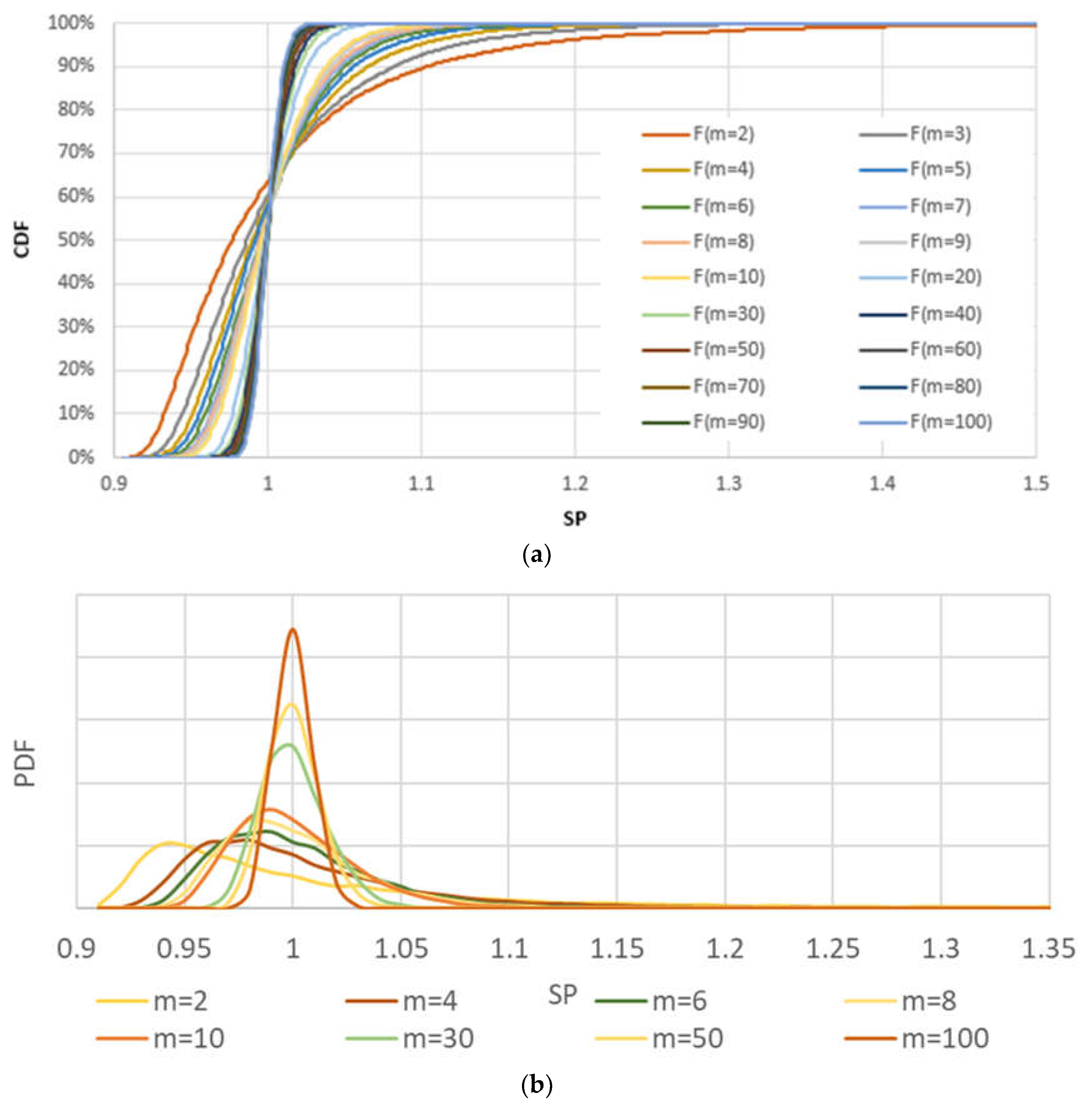
3.2.1. The Case Described in Section 2.2.1

In general, the process is clear. We simulate four pieces of data according to the normal, uniform, or other assumed distribution and compare the calculated SP and the SP_(1−α) percentile or, alternatively, calculate the corresponding p–value. In our case, the SP_0.95 percentile equals 3.43 (assuming normal, uniform, or exponential distribution; see also Figure 7) and the p–value is 10.6%. Accordingly, the conclusion is that the available data are not enough, i.e., are insufficient, to establish that products supplied by two suppliers differ in their reliability level.

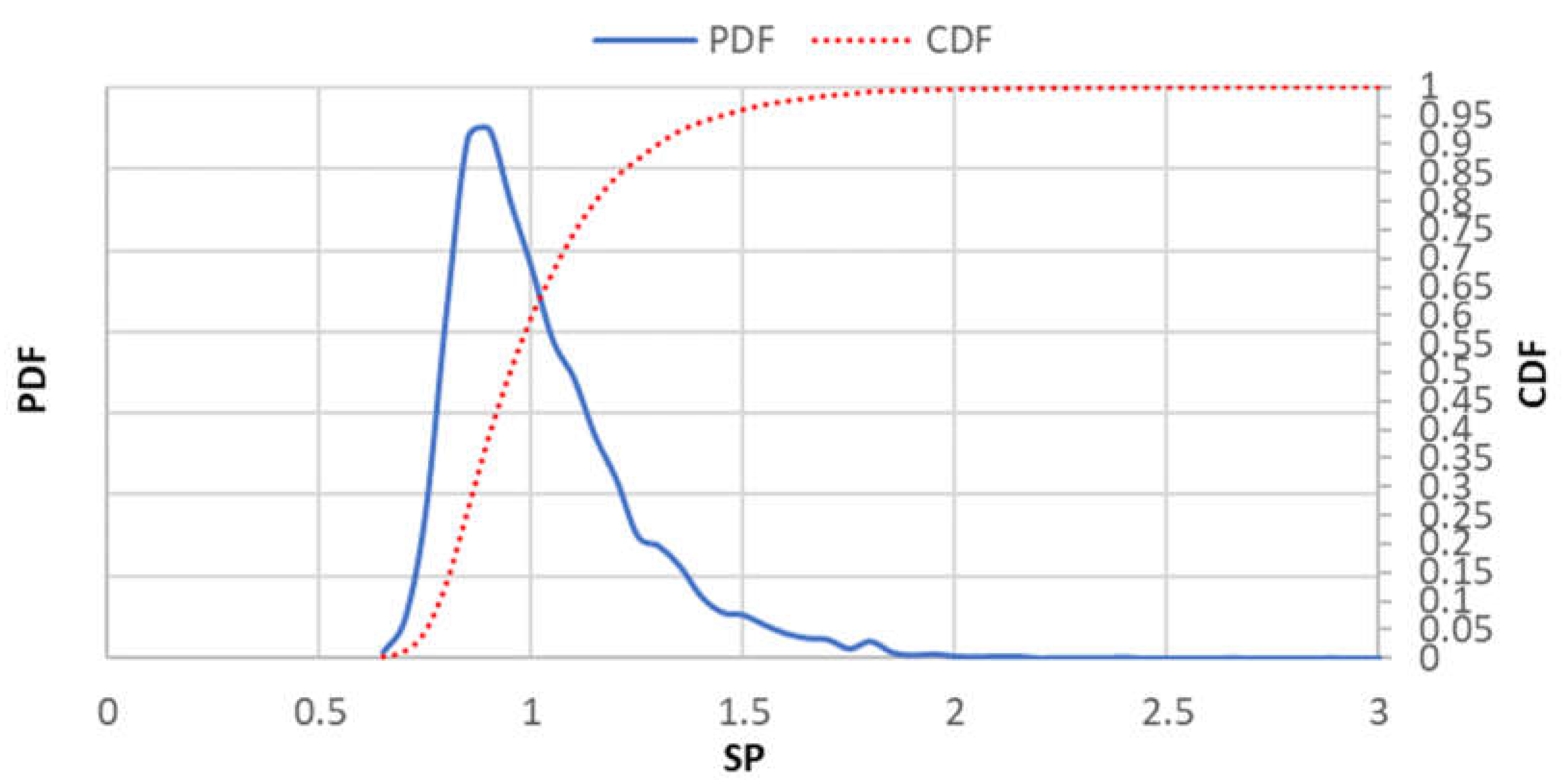
3.2.2. The Case Described in Section 2.2.2

The H₀ hypothesis determines the distribution of the categories’ proportions. In the simplest, binary case, for example, this may be the expected proportions of satisfactory and faulty products in a supplied batch of a certain size N. Let us assume that all batches are the same size and that the null hypothesis H₀ assumes the same level of quality from all suppliers. In this case, one can use the binomial (and in the general case, the multinomial) distribution for simulating the number/proportion of satisfactory and faulty products in a batch.

Let us further assume that batch sizes can vary from supplier to supplier. In this case, for the simulation, we need the Beta distribution of the proportions of bad (or good) items or, in the general multicategory case, the Dirichlet distribution Dir(γ). The latter is a continuous multivariate probability distribution parameterized by a vector $\mathit{\gamma }=({\gamma }_1,{\gamma }_2,\dots ,{\gamma }_r)$ of positive reals and is known as the multivariate generalization of the Beta distribution that describes the bivariate case only. The procedure for determining the parameters of these distributions (out of the scope of this article) is based on preliminary information (both theoretical and experimental) and is described in detail in [17]. We restrict ourselves to saying that the more accurate the preliminary information, the smaller the scale parameter that determines the variance of the simulated data. Unfortunately, in [9], which is where the example given in Section 2.2.3 is taken from, such preliminary information (total cost of quality at each company) is missing, thus making it impossible to formulate H₀.

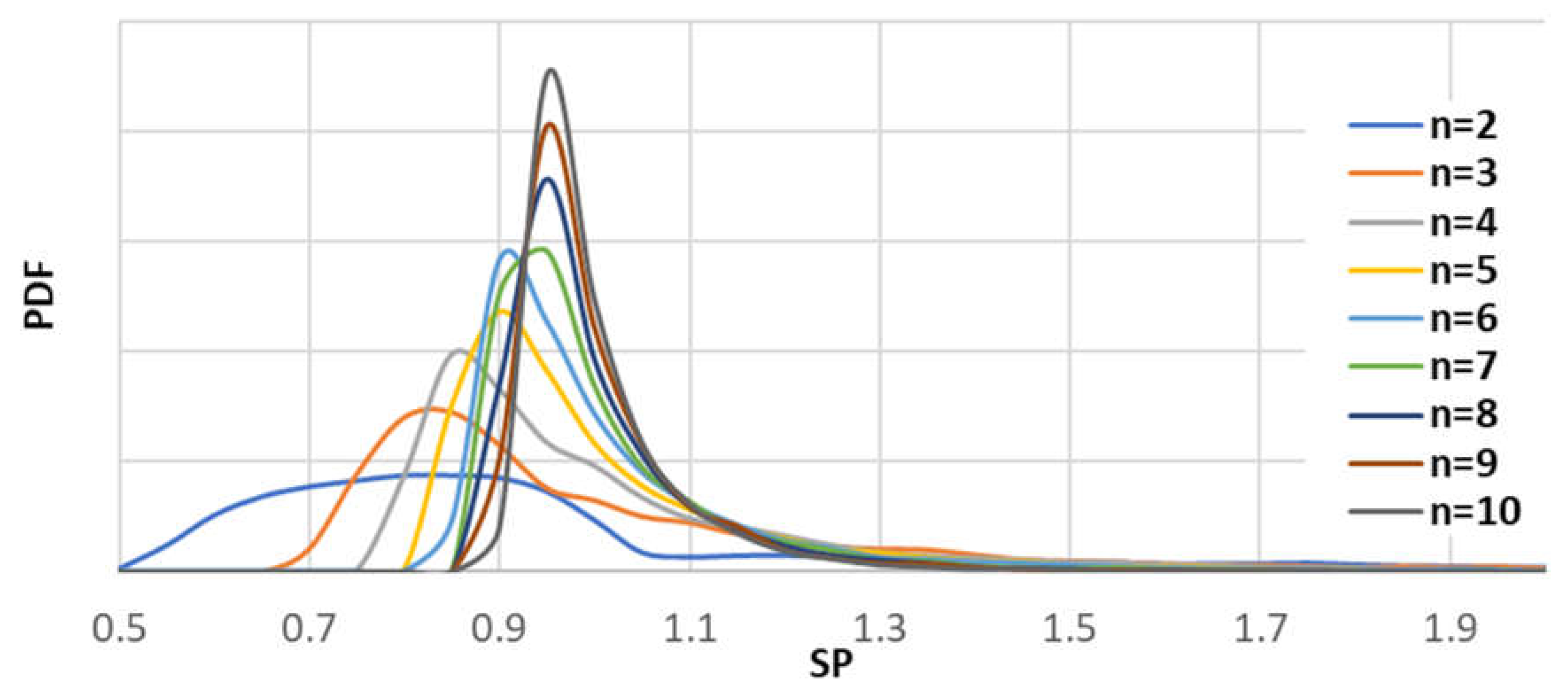
3.2.3. The Case Described in Section 2.2.3

In this example, gender equality and the absence of real preferences between alternatives were chosen as the null hypothesis H₀.

The SP distribution under this assumption for the (2,3) partition (see Figure 5) is shown in Figure 10. For α = 5%, the critical SP_0.95 = 1.476 and the p–value for the calculated SP = 1.502 equals 4.39%. Thus, we can conclude that gender has a small effect on preferences.

Another type of assumed distribution may be the so-called Mallow’s distribution, according to which preference chains are dispersed (spread) around a certain dominant preference chain serving as a “gold standard”. We refer the readers to [12] for details.

3.3. General Methodology: Modus Operandi for Analyzing a Metric Data Partition (10 Steps)

• Decide on the OUS population.
• Make an assumption about the type of the expected distribution of these objects within a homogeneous population.
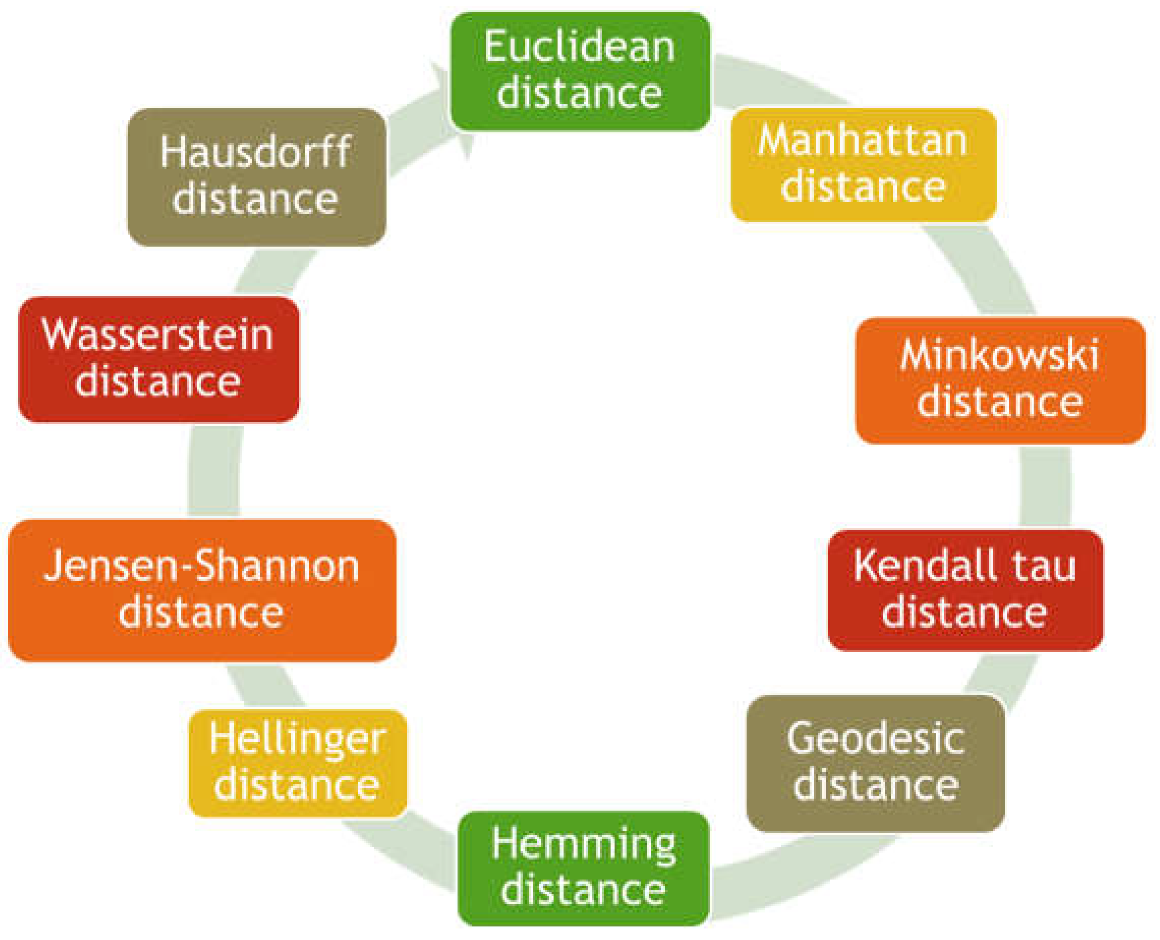
• Choose a distance metric suitable for this distribution (see Figure 1).
• Decide on the factor that, in your opinion, can discriminate/distinguish between the OUSs (heterogeneity hypothesis), and which levels serve as the basis for dividing/separating objects into groups (partitioning).
• Provide a corresponding data partitioning/division.
• Calculate the SP (as in Section 3, for example)
• Simulate the SP distribution under H₀ in accordance with the vector of the partition just made $(n_1, n_2, \dots ,n_k,\dots ,n_m)$ and the chosen distance metric. Every simulation process cycle includes:

  (a)

  Random generation of N data from a population of OUS (as per step 1) characterized by the assumed distribution (as per step 2).

  (b)

  Distance matrix calculation (as per step 3).

  (c)

  Partitioning these distances into their inter and intra components (as per steps 4 and 5).

  (d)

  SP calculation, which ends the cycle and returns us to (a).

• Determine the alpha risk α of homogeneity hypothesis H₀ rejection.
• Find the (1 − α) percentile of the simulated SP distribution, or alternatively, the p–value of the calculated SP.
• Make a final decision according to the results of step 9.

4. Discussion

This article continues the theme previously raised by a number of authors about processing new types of quality and reliability data and related problems [1,2,3,4,5].

The main goal of clustering OUS is to divide them into distinctively dissimilar but internally homogeneous groups. Such partitioning makes sense only if inter group differences significantly exceed intra group differences. This task becomes markedly easier when the difference between OUS can be expressed using a distance metric. In this case, we suggest that the verification of the correctness of the partition according to a certain criterion (for example, the level of a potentially influencing factor) can be carried out by comparing the average inter group and intra group distances. More precisely, the authors propose to use a ratio between these distances they call separation/segregation power (SP) as an indicator of such a comparison.

It is well known that even in a homogeneous population, objects are not absolutely identical, but differ due to random, noisy disturbances/perturbations (the so-called null hypothesis H₀). This, in turn, means that even for a homogeneous population, the distances between objects are neither zero nor constant; rather, they are characterized by a certain distribution, the type and parameters of which can be very different depending on the OUS. Usually, these distributions are characterized by a so-called scale parameter, to which the mean distance is proportional. The SP distribution, as shown in the paper, however, is insensitive to this as well as to any location parameter.

For a given H₀ about the behavior of a homogeneous set of OUS, the SP distribution depends only on the kind of partitioning (partition vector). Its universal theoretical analysis is barely possible because of, among other reasons, the fact that two distances with a common datum are correlated. Nevertheless, it can be calculated by simulation methods (step 7 in Section 3.3).

Three examples of different OUS and corresponding SP distributions under the H₀ are discussed in the article. As the amount of data increases, the mean SP tends to be 1, and the distribution itself narrows.

The location of the calculated SP value compared to its distribution under the H₀ makes it possible to draw a conclusion about the expediency of the generated partition and its discrimination/separation/segregation power using standard statistical methods (comparing SP_calculated to SP_1−α or the p-value to the α risk).

Though the proposed approach (see the general methodlogy in Section 3.3) is similar in spirit to ANOVA, it is innovative in that it is applicable to any type of object whose dissimilarity can be described by means of a distance metric: pie charts, prioritization chains, strings, tree structured data, etc. A certain disadvantage is the need to conduct a simulation study of the SP distribution when partitioning different kinds of OUS and the type of their spread in a homogeneous population as described in Section 3.3 (step 7). One way to circumvent this issue would be by creating a bank of such calculators along the lines of those given in [18].

We hope that the potential inherent in the analysis of metric space quality/reliability data provided here will inspire reliability engineers to explore other territories such as data-collecting sensor systems [19], clustering, discriminant analysis, experimental design, and so on. We hope that this work will serve as a catalyst for the development of new methodologies where data-driven conclusions will become the driving force of the investigation.

References

- Marmor, Y.N.; Bashkansky, E. Processing new types of quality data. Qual. Reliab. Eng. Int. 2020, 36, 2621–2638. [Google Scholar] [CrossRef]
- Song, W.; Zheng, J. A new approach to risk assessment in failure mode and effect analysis based on engineering textual data. Qual. Eng. 2024. [Google Scholar] [CrossRef]
- González del Pozo, R.; Dias, L.C.; García-Lapresta, J.L. Using Different Qualitative Scales in a Multi-Criteria Decision-Making Procedure. Mathematics 2020, 8, 458. [Google Scholar] [CrossRef]
- Weiß, C.H. On some measures of ordinal variation. J. Appl. Stat. 2019, 46, 2905–2926. [Google Scholar] [CrossRef]
- Grzybowski, A.Z.; Starczewski, T. New look at the inconsistency analysis in the pairwise-comparisons-based prioritization problems. Expert. Syst. Appl. 2020, 159, 113549. [Google Scholar] [CrossRef]
- Yang, W.; Chen, J.; Zhang, C.; Paynabar, K. Online detection of cyber-incidents in additive manufacturing systems via analyzing multimedia signals. Qual. Reliab. Eng. Int. 2022, 38, 1340–1356. [Google Scholar] [CrossRef]
- Gadrich, T.; Bashkansky, E.; Zitikis, R. Assessing variation: A unifying approach for all scales of measurement. Qual. Quant. 2015, 49, 1145–1167. [Google Scholar] [CrossRef]
- Feigenbaum, A.V. Total Quality Control, 3rd ed.; McGraw Hill: New York, NY, USA, 1991. [Google Scholar]
- Rosenfeld, Y.; Jabrin, H.; Baum, H. Costs of Non-Qualiy in Residential Construction in Israel; National Institute for Construction Research: Haifa, Israel, 2019. Available online: https://www.gov.il/BlobFolder/reports/research_1077/he/r1077.pdf (accessed on 16 July 2023). (In Hebrew)
- Le Cam, L.M.; Yang, G.I. Asymptotics in Statistics: Some Basic Concepts; Springer Science & Business Media: New York, NY, USA, 2000. [Google Scholar] [CrossRef]
- Vanacore, A.; Marmor, Y.N.; Bashkansky, E. Some metrological aspects of preferences expressed by prioritization of alternatives. Measurement 2019, 135, 520–526. [Google Scholar] [CrossRef]
- Marmor, Y.N.; Gadrich, T.; Bashkansky, E. Accuracy of multiexperts’ prioritization under Mallows’ model of errors creation. Qual. Eng. 2021, 33, 286–299. [Google Scholar] [CrossRef]
- McKay, A.T.; Pearson, E.S. A note on the distribution of range in samples of n. Biometrika 1933, 25, 415–420. [Google Scholar] [CrossRef]
- Hartley, H.O. The range in random samples. Biometrika 1942, 32, 334–348. [Google Scholar] [CrossRef]
- Crooks, G.E. Field Guide to Continuous Probability Distributions; Berkeley Institute for Theoretical Science: Berkeley, CA, USA, 2019; Available online: https://threeplusone.com/pubs/FieldGuide.pdf (accessed on 16 July 2023).
- Johnson, H.L.; Kotz, S.; Balakrishnan, N. Continuous Univariate Distributions, 2nd ed.; John Wiley & Sons: New York, NY, USA, 1994. [Google Scholar]
- Gadrich, T.; Bashakansky, E. A Bayseian approach to evaluating uncertainty of inaccurate categorical measurements. Measurement 2016, 91, 186–193. [Google Scholar] [CrossRef]
- Gadrich, T.; Marmor, Y.N. Two-way ORDANOVA:Analyzing ordinal variation in a cross-balanced design. J. Stat. Plan. Inference 2021, 215, 330–343. [Google Scholar]
- Kumar, P.; Kumar, A. Quantifying Reliability Indices of Garbage Data Collection IOT-based Sensor Systems using Markov Birth-death Process. Int. J. Math. Eng. Manag. Sci. 2023, 8, 1255–1274. [Google Scholar] [CrossRef]
- Seltman, H. Approximations for Mean and Variance of a Ratio. Available online: https://www.stat.cmu.edu/~hseltman/files/ratio.pdf (accessed on 19 July 2019).