Modeling and Control of a DC-DC Buck–Boost Converter with Non-Linear Power Inductor Operating in Saturation Region Considering Electrical Losses

Abstract

The present work proposes a nonlinear model of a buck–boost DC-DC power converter considering the nonlinear magnetic characteristics of the power inductor and electrical losses of the system. The Euler–Lagrange formalism is used for formulating the proposed model. Previous research works have reported mathematical models to describe power inductor dynamics. However, a gap in the literature remains regarding modeling this kind of element when it operates within power converters. Also, a linear-based controller scheme is proposed to regulate a non-ideal buck–boost DC-DC power converter. A methodology for tuning the proposed controller is presented, which considers the nonlinear model structure of the power converter, the linearization procedure based on an identification process, and a frequency domain analysis based on the approximated linear model. Finally, the tuned control scheme is tested on the nonlinear model of the power converter under several operational conditions showing excellent performance by effectively regulating the output voltage. The results are compared with those derived from alternative control strategies, and a better performance is generally obtained.

1. Introduction

DC-DC power converters connect two direct current (DC) systems and efficiently control the energy flow between them [1]. The operation of these devices can reduce losses caused by the energy conversion process by controlling the state of the switchers. [2]. One way to classify DC-DC power converters is based on the relation between their input and output voltage values, which are buck, boost, and buck–boost converters [3]. The DC-DC buck–boost power converter can be applied as an actuator in various processes owing to its adaptability to function within a specified operational range. This adaptability is exemplified by its capacity to provide an output voltage that can be either higher or lower than the input voltage supplied. DC-DC buck–boost power converters are used in applications that need high flexibility for reducing or increasing voltage to a reference value [4]. These converters have been applied for supplying voltage to constant or variable loads [5], correcting the power factor in wind turbine systems, and controlling LED technology lighting circuits [6] and energy storage systems [7]. Some studies have developed mathematical models of ideal converters to describe them dynamically, as was done in [8]. Other authors have developed more realistic models considering internal electrical losses in the converter operation [9].

Power inductors are fundamental components for DC-DC buck–boost power converters [10]. Magnetic hysteresis and magnetic saturation are nonlinear phenomena that have remarkable effects on the operation of power inductors [11,12]. Several models have been developed to represent the magnetic saturation in power inductors, for example, polynomial models [13], neural models [10], models based on power behavior [14], and models based on trigonometric functions [12]. Each model has its particularities, and its use depends of the application [14]. None of these models have been applied to simulate the effects of magnetic saturation in a power inductor that operates within a buck–boost DC-DC power converter. In this research work, this gap is covered using the Euler–Lagrange formalism, which is used as a mathematical tool for integrating the inductor model described in [12] into the dynamics of a DC-DC buck–boost power converter.

Controllers are essential for regulating the power converter operation and ensuring good performance for the intended applications. Controllers have to be designed and tuned considering the characteristics of the power converter, such as their electrical losses, the nominal values of their components, and the operations that heed to be executed. Many authors have proposed controllers to regulate the operation of power converters. Linear controllers, such as the classical PI, have found application in various studies, as in [9]. Several authors have tuned the gains of the PI controller by employing a linear model of a DC-DC converter, combined with the Ziegler–Nichols tuning method, as found in [15,16]. In [17], the tuning process was developed using an identification algorithm and frequency response analysis to guarantee a robust control scheme for a buck power converter. Also, nonlinear control strategies have been considered for this purpose, such as passivity-based control (PBC) [3] and adaptive control strategy [13]. Other researchers have explored controller schemes that blend both linear and nonlinear strategies, as demonstrated in [18], where a PI controller is combined with a PBC to ensure zero error at the voltage output in the steady state.

Many of the research mentioned above, especially those related to the implementation of nonlinear control schemes, predominantly emphasize the tuning process of controllers to ensure power converter stability. However, these studies often overlook crucial aspects related to controller performance, such as robustness and transient response characteristics. Furthermore, they tend to provide a limited analysis of the nonlinear model structure used to characterize the power converter, including its relative and absolute degrees, so they leave a noticeable gap in those researches.

The main contributions are:

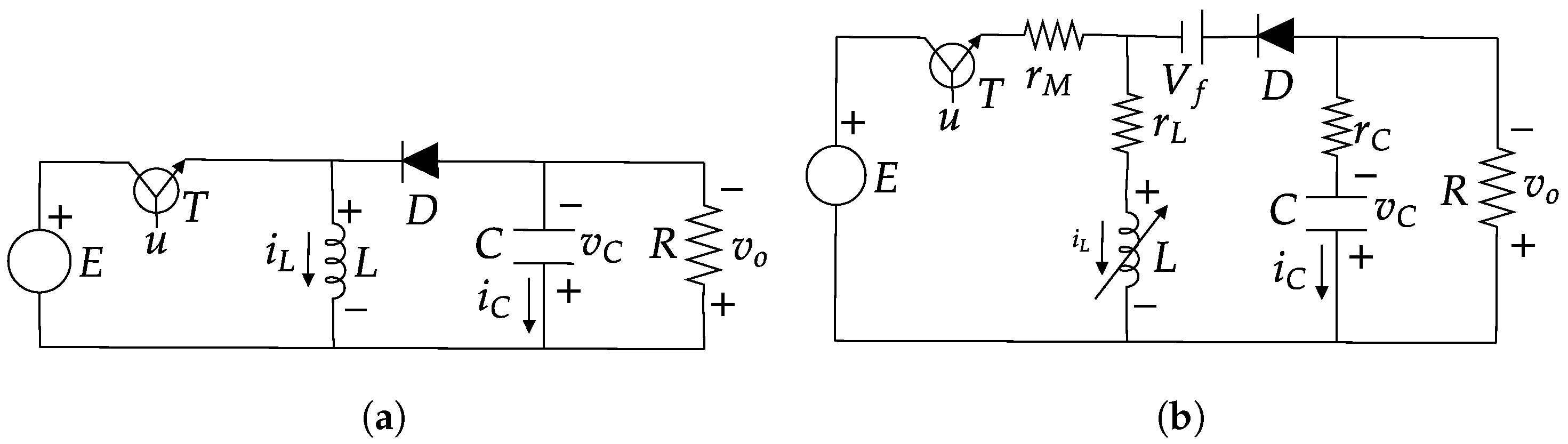
• This study introduces a mathematical model to simulate magnetic saturation effects and electrical losses in a power inductor operating in a buck–boost DC-DC converter. The model integrates a nonlinear arc-tangent-based inductor model with a converter model accounting for electrical losses. The Euler–Lagrange formalism is used for coupling those effects.
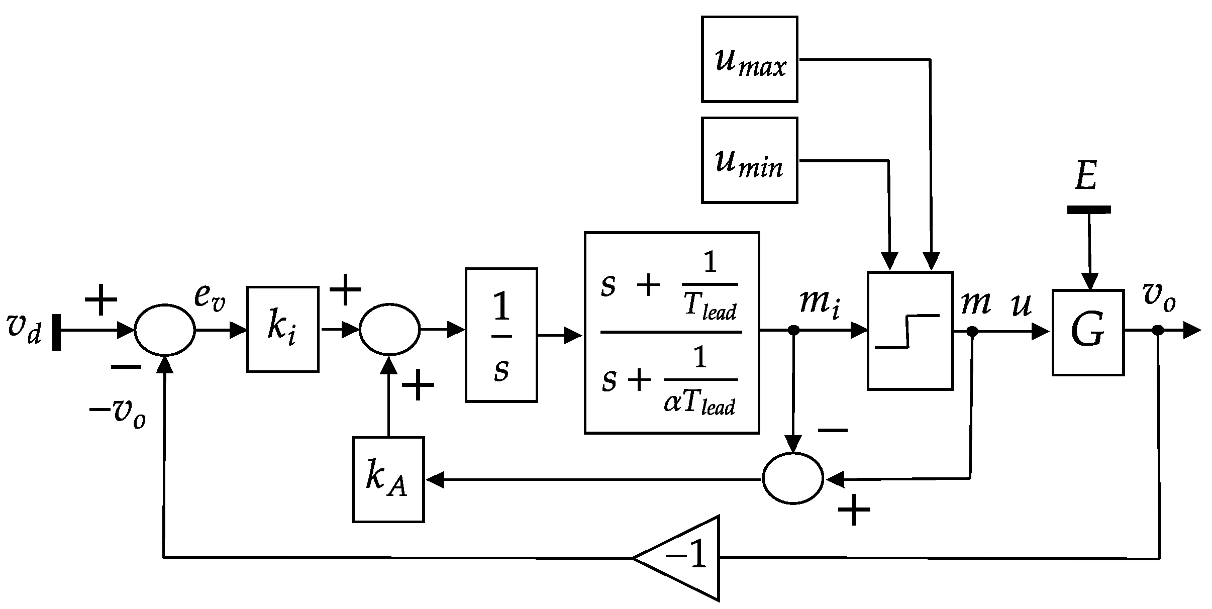
• The study suggests a simple but effective linear control strategy for voltage regulation in the converter. This method employs a standard integral controller with a lead-compensator action, combined with an anti-windup mechanism. The parameters for the anti-windup scheme are determined based on the mathematical model, specifically considering the converter behavior during steady-state operation.
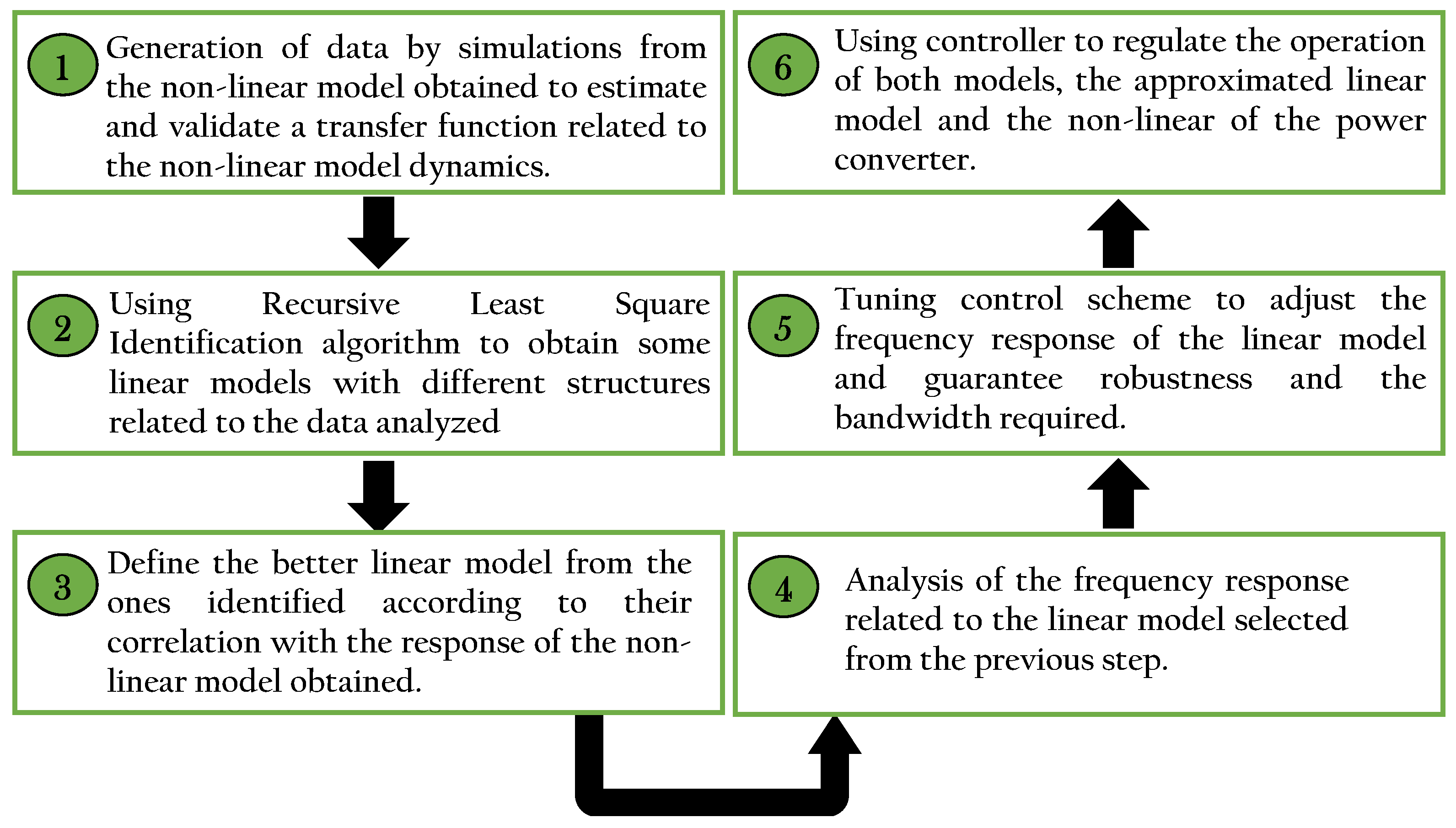
• The article introduces a comprehensive tuning procedure consisting of two primary stages. Firstly, a linearization of the non-linear model is achieved through an identification algorithm, aligning with the structure of its state–space representation. Subsequently, the generated linear model is employed to fine-tune control scheme parameters using frequency response analysis, ensuring both the stability and robustness of the controlled device.

However, the reported results in this research work are a first step focused on controlling physical buck–boost DC-DC power converters for further implementations.

The article is organized as follows: Section 2 defines the problem formulation on which the present study is based. Section 3 shows the mathematical model of an ideal DC-DC buck–boost conventional power converter and the control strategy proposed to regulate its operation. Section 4 proposes the experimentally validated mathematical expression for modeling a non-linear inductance that can operate on deep magnetic saturation region [12]. In Section 5, the space-state model of the non-ideal power converter in space state is developed. Section 6 shows the results that are compounded by the analysis of the behavior of the proposed power converter model as well as the design of the proposed control scheme and the performance of the control system. The tuning methodology is based on a linear model identification from the non-linear one using a recursive least-square algorithm and frequency response analysis of the linear model estimated. Section 7 presents a comparative analysis that contrasts the non-linear PI controller proposed in [9] and the PBC+PI approach introduced in [13], with the proposed linear controller scheme designed in this research work. Finally, conclusions are presented in Section 8.

2. Problem Formulation

The operation of the power inductor in its saturation region introduces dynamics that can compromise the performance of a DC-DC buck–boost power converter, potentially affecting its integrity. Furthermore, the presence of electrical losses within the converter is undesirable as it limits its operating range. Therefore, when designing the controller scheme for regulating the operation of the power converter, both characteristics must be considered.

The topology of an ideal DC-DC buck–boost power converter is shown in Figure 1a. The device shown is a SISO second-order system. In Figure 1, L is the inductance of the power inductor inside the converter; C is the capacitance of the integrated capacitor in the circuit; R represents the connected load to the device; D is the required diode in this circuital configuration; T is the switcher used for controlling the device operation state; and u is the excitation signal used for controlling the state of the element T, which can have discrete values $\left[0,1\right]$. This converter supplies an output voltage $v_o$ of reverse polarity concerning input voltage E.

As illustrated in Figure 1, the power converter topology has a basic structure that depends on a minimal number of electrical components. Operational versatility and structural simplicity are the primary factors behind selecting this power converter as the subject of study in the current research.

The topology presented in Figure 1b takes into account the electrical losses and non-linear characteristics of the power inductor. $r_M$ is the resistance associated with the switcher device T, $r_L$ is the inductor coil resistance, $r_C$ represents capacitor operation losses, $V_f$ is the drop voltage on the diode when it is activated, and inductance L is a non-linear parameter that depends on the magnetic permeability.

3. Modeling and Control of an Ideal DC-DC Buck–Boost Converter

3.1. Mathematical Model of an Ideal DC-DC Buck–Boost Power Converter

The circuits shown in Figure 2 represent the power converter operation in their different states. These are used to generate the model of the ideal power converter. The circuit of Equation (1a) is valid when the converter switcher is on while the circuit of Equation (1b) is used when the switcher is off.

The energy equations related to the circuit represented by Figure 2a are the following:

$${\mathcal{T}}_{u=1}\left({\dot{q}}_L\right)=\frac{1}{2}L{\dot{q}}_L^2$$

(1a)

$${\mathcal{U}}_{u=1}\left(q_C\right)=\frac{1}{2C}{q}_C^2$$

(1b)

$${\mathcal{F}}_{q_C}^{u=1}=0$$

(1c)

$${\mathcal{F}}_{q_L}^{u=1}=E$$

(1d)

$${\mathcal{D}}_{u=1}\left({\dot{q}}_C\right)=\frac{1}{2}R{\dot{q}}_C^2$$

(1e)

The energy equations related to the circuit represented by Figure 2b are shown in the relation Equation (2):

$${\mathcal{T}}_{u=0}\left({\dot{q}}_L\right)=\frac{1}{2}L{\dot{q}}_L^2$$

(2a)

$${\mathcal{U}}_{u=0}\left(q_C\right)=\frac{1}{2C}{q}_C^2$$

(2b)

$${\mathcal{F}}_{q_L}^{u=0}=0$$

(2c)

$${\mathcal{F}}_{q_C}^{u=0}=0$$

(2d)

$${\mathcal{D}}_{u=0}({\dot{q}}_L,{\dot{q}}_C)=\frac{1}{2}R{({\dot{q}}_L+{\dot{q}}_C)}^2$$

(2e)

$\mathcal{T}$ is the circuit kinetic energy, which is caused for stored energy in the power inductor; $\mathcal{U}$ is the potential energy related to the stored energy in the capacitor; $\mathcal{D}$ represents elements that generate heat not reusable for the device; and $\mathcal{F}$ represents all the signals that excite the system in such a way that its state of operation has changed. The $\mathcal{D}$ and $\mathcal{F}$ terms are defined as generalized forces [3].

Using the energy expressions in the Euler–Lagrange formalism, the ideal converter dynamical model is given by:

$$L\frac{d}{dt}{i}_L=(1-u)v_C+uE$$

(3a)

$$C\frac{d}{dt}{v}_C=-(1-u)i_L+\frac{1}{R}{v}_C$$

(3b)

The state variables are the inductor current $i_L$ and capacitor voltage $v_C$. Equation (3a,b) are the space representation of an averaging model where u can have continuous values belonging to the interval $\left[0;1\right)$[9]. Input voltage E is considered a constant value, while u is the signal that regulates the converter operation. The obtained ideal converter model is nonlinear, as can be seen in Equation (3a,b). The following relation represents the system output variable:

$$v_o=v_C$$

(4)

3.2. Proposed Controller Scheme

The control law employed to regulate the operation of the power converter is founded on the adjustment of the duty cycle of the PWM signal, denoted as u, which is applied to the gate of the circuit switcher, for the purpose of governing its voltage output. The controller characterized by the relation Equation (5) is the basis of the proposed control scheme.

$$M\left(s\right)=\alpha k_i\frac{T_{lead}s+1}{s\left(\alpha T_{lead}s+1\right)}E\left(s\right)$$

(5)

The controller is structured by an I action with a lead-compensator, where $k_i$ is the gain associated with the integral action, $T_{lead}$ is the time associated with the lead-compensation action, and $\alpha$ is the coefficient of the lead compensation action. $E\left(s\right)$ is the voltage tracking error, and it is obtained from Equation (6), from which $V_d^{*}\left(s\right)$ is the desired output voltage and $V_o\left(s\right)$ is the converter output voltage. $M\left(s\right)$ is the command signal generated by the controller and is related to the duty cycle used as a signal to adjust the operation of the power converter switcher.

$$E\left(s\right)=V_d^{*}\left(s\right)-V_o\left(s\right)$$

(6)

The duty ratio generated by the controller to regulate the power converter must be restricted to the interval $m\in (0;1)$ because if it is not, the system will revert to operating conditions that are incompatible with the averaging mathematical model [9]. In the study performed in [19], the authors experimentally validated that the maximum effective duty ratio of a real DC-DC buck–boost power converter is lower than one. The range of u depends on the electrical losses of the device. This result means that this control signal is effective in a range that is less than ideal. If this consideration is not regarded, some issues related to the stability of the controlled device may be generated. The maximum value associated with this range can be computed considering the nonlinear model behavior of the power converter operating in the stationary state along the whole ideal range of values for the control input u.

The valid operational range for u can be achieved by saturating the control signal inside this interval. However, one pitfall of this strategy is that, as is well known, a controller with an integral action and control signal saturation can lead to instability. These adverse effects of the saturation over the integral action can be avoided using an anti-windup scheme coupled to the proposed linear controller. Many authors used this methodology to implement their controllers in processes that have some restrictions over the command signal [20,21].

The scheme proposed for the linear controller is shown in Figure 3, where it is necessary that $v_d\ge 0$. In the scheme control, $k_A$ is the gain associated with the anti-windup strategy, and $u_{max}$ and $u_{min}$ are the limits of control signal saturation.

3.3. Methodology for Tuning the Linear Controller

The tuning of the proposed controller is made by adjusting the $k_i$ gain, the $\alpha$ coefficient, and the $T_{lead}$ term to satisfy the desired response of the power converter. This response has to be robust against parametric variations. Frequency analysis is an easy way to ensure stability, robustness, and performance by means of the gain and phase margins [22]. However, this requires linear models for its application. Therefore, an approximated linear model of the non-linear one is required. One way to achieve this linear model is via an identification procedure, as in [17].

As a first step, the input/output data of the non-linear non-ideal power converter model is required, generated within the practical duty cycle ratio. The second step is to estimate and validate a linear model that can represent the non-linear model dynamics. In this phase, it is essential to establish the structure of the linear model to be employed, which is determined by the absolute and relative degree associated with the nonlinear system.

The linear controller is designed and tuned based on the frequency analysis of the obtained linear model in such a way that the gain and phase margins are large enough to guarantee robust stability. Another characteristic to consider in the design process is the bandwidth of the controlled system, which is related to the response of the controlled converter.

Finally, the controller is evaluated based on the analysis of the time responses of the control system, throughout a wide operating range, using converter nonlinear model. Figure 4 summarizes the entire process.

Additionally, the performance of the proposed controller scheme is compared to other schemes based on their time responses. The comparison also takes into account controller complexity and the number of required feedback signals for regulation.

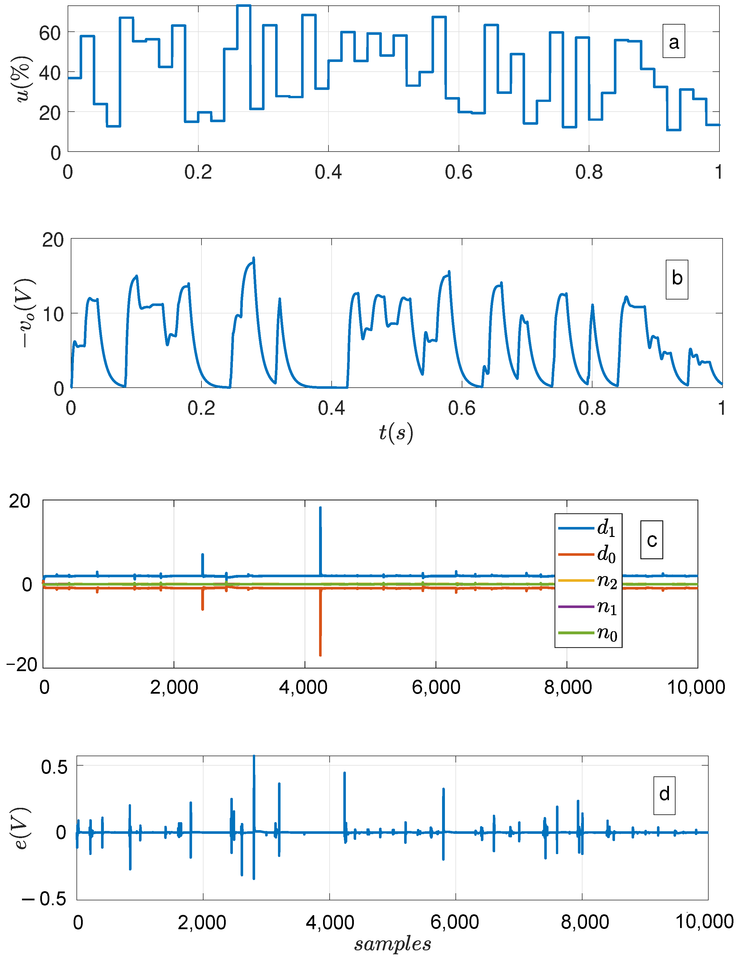
3.4. Recursive Least-Square Identification Algorithm

The recursive least-square identification algorithm is used to identify the dynamics of discrete processes [23]. This algorithm was used in previous studies to fit transfer functions in the z-domain considering a set of sampled data as in [24]. Consider the strictly proper discrete transfer function as the following expression:

$$G\left(z\right)=\frac{Y\left(z\right)}{U\left(z\right)}=\frac{b_m{z}^{m-n}+\cdots +b_0{z}^{-n}}{1+a_{n-1}{z}^{-1}+\cdots +a_1{z}^{-n+1}+a_0{z}^{-n}}$$

(7)

where $m,n\in \mathbb{N}$; $m\le n$. $Y\left(z\right)$; and $U\left(z\right)$ are the system output and input, respectively. The difference equation associated with the previous transfer function can be expressed as:

$$y_r\left(k\right)=-(a_{n-1}y(k-1)+\cdots +a_{1}y(k-n+1)+a_{0}y(k-n))+(b_{m}u(k-n+m)+\cdots +b_{0}u(k-n))$$

(8)

$y_r\left(k\right)$ is the real output of the system in a kth sample instant, with $k\in Z$. Expressing the difference equation in vectorial form:

$$y_r\left(k\right)={\theta }_r^T\varphi (k-1)$$

(9)

the term ${\theta }_r$ represents the real parameters associated with the dynamic of the system and corresponds to the form:

$$\theta ={[-a_{n-1}-a_{n-2}\cdots -a_1-a_0{b}_m\cdots b_0]}^T$$

(10)

and $\varphi (k-1)$ is the observed data vector and is equivalent to the next vector:

$$\varphi (k-1)={[y(k-1)\dots y(k-n)u(k-n+m)\dots u(n-m)]}^T$$

(11)

In a practical model based on the difference equation, the previous expression can be expressed by adding a noise component generated by the normal operation of the sensor. In this paper, the noise is not considered because the study was carried out based on simulation tests. There are some methods used for identifying the dynamics of practical systems as the use of noise and/or the perturbation observer, as was done in [23].

During the identification process, the real and the estimated outputs are compared.

$$e\left(k\right)=y_e\left(k\right)-y_r\left(k\right)$$

(12)

where $y_e\left(k\right)$ is the estimated output generated by the identification algorithm and $e\left(k\right)$ is the error between $y_r\left(k\right)$ and $y_e\left(k\right)$. The aim of the identification algorithm is minimize the estimation error. The estimated output can be obtained by the following vectorial expression:

$$y_e\left(k\right)={\theta }_e^T\varphi (k-1)$$

(13)

where ${\theta }_e$ is the vector compounded by the estimated coefficients. The vectors ${\theta }_r$ and ${\theta }_e$ must have the same structure to guarantee the convergence of the identification algorithm; then, it is required to know the absolute degree and the relative degree associated with the dynamics of the system analyzed.

The ${\theta }_e$ vector has to be estimated from the observed data in a recursive way to minimize the cost function $\mathcal{J}=e{\left(k\right)}^2$ [23]. This goal can be achieved using the quadratic criteria Equation (14):

$$\mathcal{J}\left({\theta }_e\left(i\right)\right)=\sum _{i=1}^k\left(\prod _{j=1}^k\lambda \left(j\right)\right)e{\left(i\right)}^2$$

(14)

where $\lambda \left(k\right)$ is a pondered constant value for all k domain. This value is defined as the forgetting factor of the algorithm [25]. The term $\lambda$ must be included inside the interval $(0;1]$. The development of Equation (14) to obtain its minimum value allows us to obtain the following equations to fit the model parameters based on the observed data [26]:

$${\theta }_e\left(k\right)={\theta }_e(k-1)+\lambda F(k+1)\varphi (k-1)e\left(k\right)$$

(15a)

$$e\left(k\right)=y_r\left(k\right)-{\theta }_r{(k-1)}^T\varphi (k-1)$$

(15b)

$$F(k+1)=\frac{1}{\lambda }\left(F\left(k\right)-\frac{F\left(k\right)\varphi (k-1)\varphi {(k-1)}^{T}F\left(k\right)}{1+\varphi {(k-1)}^{T}F\left(k\right)\varphi (k-1)}\right)$$

(15c)

the matrix $F\left(k\right)$ is a co-variance one and must be positive definite for achieving convergence of the identification method.

The recursive least-square identification algorithm with the forgetting factor converges in the situation associated with the present study if the following conditions are satisfied:

• The number of poles and zeros of the function to be modeled are already known. Then, the structure of ${\theta }_e$ and ${\theta }_r$ must be similar.
• $u\left(k\right)$ is a persistent excitation signal.
• $u\left(k\right)$ and $y\left(k\right)$ must be bounded.

This identification method will be use to obtain a linear model that closely approximates the non-linear behavior of the DC-DC buck–boost power converter.

4. Non-Linear Inductance Model

One of the nonlinearities in the power inductor operation is magnetic saturation, which can be categorized into three types: oscillating inductor saturation; partial saturation, further divided into weak, deep and roll-off regions; and full saturation. This magnetic phenomenon produces variations in the inductance of the power inductor under certain operational conditions. The effective inductance is represented as [11]:

$$L(i,T)=\frac{\partial }{\partial i}\mathsf{\Phi }(i,T)$$

(16)

which depends on the magnetic flux variation related to the operational temperature of the inductor core and coil current [12]. The stored energy expression in the inductor considering a constant value in the temperature is determined by the following expression [11]:

$$E_L=\int \mathsf{\Phi }\left(i_L\right)d{i}_L=\int L\left(i_L\right)i_{L}d{i}_L$$

(17)

Non-linear inductance relies on several factors. In [12], an arc-tangent-based model is introduced to represent the inductance-power inductor current relationship. The present research employs this model to explore the behavior of the power inductor as the current $i_L$ varies. The choice of this model is justified by its versatility, capable of describing inductance behavior across a wide range of $i_L$ values, including deep saturation. In contrast, other models, such as polynomial-based models, are limited to specific operational regions. Additionally, the arc-tangent model simplifies the tuning process as it relies solely on manufacturer-provided data, reducing tuning complexity compared to other models.

The equation provided defines the arc-tangent-based model for a power inductor, which was empirically tested by [12]:

$$L\left(i_L\right)=L_d+\frac{L_n-L_d}{2}\left[1-\frac{2}{\pi }arctan\left[\sigma (i_L-I_L)\right]\right]$$

(18)

where:

• $L_n$: The horizontal asymptote parameter related to the maximum inductance value when operated on the weak saturation region. This parameter is equal to the nominal inductance value provided by its manufacturer.
• $L_d$: The horizontal asymptote parameter related to the minimum inductance value when operated on the deep saturation region. This parameter is obtained from the data provided by the inductor manufacturer.
• $\sigma$: This factor represents the roll-off region behavior between both defined saturation regions.
• $I_L$: This parameter is the current when the element inductance is equal to the average value between $L_n$ and $L_d$.

The $\sigma$ and $I_L$ parameters can be obtained using the inductor performance curves provided by the manufacturer related to the terminal current. The following expressions determine these parameters:

$$I_L=\frac{I_{x_2}cot\left(\pi {\Gamma }_{x_1}\right)-I_{x_1}cot\left(\pi {\Gamma }_{x_2}\right)}{cot\left(\pi {\Gamma }_{x_1}\right)-cot\left(\pi {\Gamma }_{x_2}\right)}$$

(19a)

$$\sigma =\frac{cot\left(\pi {\Gamma }_{x_1}\right)-cot\left(\pi {\Gamma }_{x_2}\right)}{I_{x_2}-I_{x_1}}$$

(19b)

where the relations $x_1<x_2$, $x_1>10\%$ and $x_2<90\%$ should be satisfied. $I_x$ is the required current for the inductance that may equal $x{L}_n$. The parameter ${\Gamma }_x$ is calculated as:

$${\Gamma }_x=\frac{L_x-L_d}{L_n-L_d}$$

(20)

5. Non-Ideal DC-DC Buck–Boost Power Converter Proposed Model

The circuits shown in Figure 5 are proposed to model the non-ideal DC-DC buck–boost power converter.

The following equations are related to the energy storage in the circuits elements of Figure 5a:

$${\mathcal{T}}_{u=1}\left({\dot{q}}_L\right)=\int L\left({\dot{q}}_L\right){\dot{q}}_L$$

(21a)

$${\mathcal{U}}_{u=1}\left(q_C\right)=\frac{1}{2C}{q}_C^2$$

(21b)

$${\mathcal{F}}_{q_L}^{u=1}=E$$

(21c)

$${\mathcal{F}}_{q_C}^{u=1}=0$$

(21d)

$${\mathcal{D}}_{u=1}({\dot{q}}_L,{\dot{q}}_C)=\frac{1}{2}\left((r_M+r_L){\dot{q}}_L^2+(R+r_C){\dot{q}}_C^2\right)$$

(21e)

for the circuit of Figure 5b:

$${\mathcal{T}}_{u=0}\left({\dot{q}}_L\right)=\int L\left({\dot{q}}_L\right){\dot{q}}_L$$

(22a)

$${\mathcal{U}}_{u=0}\left(q_C\right)=\frac{1}{2C}{q}_C^2$$

(22b)

$${\mathcal{F}}_{q_L}^{u=0}=-V_f$$

(22c)

$${\mathcal{F}}_{q_C}^{u=0}=0$$

(22d)

$${\mathcal{D}}_{u=0}({\dot{q}}_L,{\dot{q}}_C)=\frac{1}{2}\left(r_L{\dot{q}}_L^2+r_C{\dot{q}}_C^2+R{({\dot{q}}_L+{\dot{q}}_C)}^2\right)$$

(22e)

The subsequent relations allow one to rewrite the energy Equations (21) and (22), considering that the control signal u is continuous and satisfies the condition $u\in \left[0,1\right]$.

$${\mathcal{T}}_u\left({\dot{q}}_L\right)=\int L\left({\dot{q}}_L\right){\dot{q}}_L$$

(23a)

$${\mathcal{U}}_u\left(q_C\right)=\frac{1}{2C}{q}_C^2$$

(23b)

$${\mathcal{F}}_{q_L}^u=uE-(1-u)V_f$$

(23c)

$${\mathcal{F}}_{q_C}^u=0$$

(23d)

$${\mathcal{D}}_u({\dot{q}}_L,{\dot{q}}_C)=\frac{1}{2}\left((u{r}_M+r_L){\dot{q}}_L^2+r_C{\dot{q}}_C^2+R{((1-u){\dot{q}}_L+{\dot{q}}_C)}^2\right)$$

(23e)

The Lagrangian function representing the analyzed device is equivalent to the following expression:

$$\mathcal{L}({\dot{q}}_L,q_C)={\mathcal{T}}_u\left({\dot{q}}_L\right)-{\mathcal{U}}_u\left(q_C\right)=\int L\left({\dot{q}}_L\right){\dot{q}}_L-\frac{1}{2C}{q}_C^2$$

(24)

The terms $q_C$ and $q_L$ are the system generalized coordinates, where $q_C$ is the instantaneous charge in the capacitor, and $q_L$ is related to the charge of the inductor. When Equation (18) is coupled with the Lagrangian, then the following relations arise from the Euler–Lagrange formalism application:

$$\frac{\partial \mathcal{L}}{\partial {\dot{q}}_L}=\frac{\partial \left(\int \left(L\left({\dot{q}}_L\right){\dot{q}}_{L}d{\dot{q}}_L\right)\right)}{\partial {\dot{q}}_L}=L\left({\dot{q}}_L\right){\dot{q}}_L$$

(25a)

$$\frac{d}{dt}\left(\frac{\partial \mathcal{L}}{\partial {\dot{q}}_L}\right)=L_{eq}\left(i_L\right){\ddot{q}}_L=L\left({\dot{q}}_L\right){\ddot{q}}_L+\dot{L}\left({\dot{q}}_L\right){\dot{q}}_L$$

(25b)

$$\frac{\partial \mathcal{L}}{\partial q_L}=0$$

(25c)

$${\mathcal{F}}_{q_L}^u=uE+(1-u)V_f$$

(25d)

$$\frac{\partial {\mathcal{D}}_u}{\partial {\dot{q}}_L}=(u{r}_M+r_L){\dot{q}}_L^2+(1-u)R\left[(1-u){\dot{q}}_L+{\dot{q}}_C\right]$$

(25e)

$$\frac{\partial \mathcal{L}}{\partial q_C}=-\frac{q_C}{C}$$

(26a)

$$\frac{d}{dt}\left(\frac{\partial \mathcal{L}}{\partial {\dot{q}}_C}\right)=\frac{\partial \mathcal{L}}{\partial {\dot{q}}_C}=0$$

(26b)

$${\mathcal{F}}_{q_C}^u=0$$

(26c)

$$\frac{\partial {\mathcal{D}}_u}{\partial {\dot{q}}_C}=r_C{\dot{q}}_C+R\left[(1-u){\dot{q}}_L+{\dot{q}}_C\right]$$

(26d)

Defining $i_L={\dot{q}}_L$ and $v_C=C{q}_C$, the dynamical model of the non-ideal converter can be represented by the next set of equations:

$$L_{eq}\frac{d}{dt}{i}_L\left(t\right)=-\left[u{r}_M+r_L+\frac{R{r}_C}{R+r_C}{(1-u)}^2\right]i_L+\frac{R}{R+r_C}(1-u)v_C+u(E+V_f)-V_f$$

(27)

$$C\frac{d}{dt}{v}_C\left(t\right)=-\frac{R}{R+r_C}(1-u)i_L-\frac{v_C}{R+r_C}$$

(28)

The following expression obtains the converter output voltage:

$$v_o=\frac{R}{R+r_C}{v}_C-\frac{R{r}_C}{R+r_C}(1-u)i_L$$

(29)

The expression Equation (25b) can be rewritten as:

$$L_{eq}\left(i_L\right)\frac{d{i}_L}{dt}=L\left(i_L\right)\frac{d{i}_L}{dt}+i_L\frac{dL\left(i_L\right)}{dt}$$

(30)

Therefore, the expression of $L_{eq}\left(i_L\right)$, when all the above conditions are considered in the inductor operation, is the following:

$$L_{eq}\left(i_L\right)=L\left(i_L\right)+i_L\frac{dL\left(i_L\right)}{d{i}_L}$$

(31)

The term $\frac{dL\left(i_L\right)}{d{i}_L}$, taking into account the function in Equation (18), is equivalent to the following expression:

$$\frac{dL\left(i_L\right)}{d{i}_L}=\frac{L_d-L_n}{\pi }\frac{\sigma }{{\sigma }^2{(i_L-I_L)}^2+1}$$

(32)

Then, Equation (31) can be formulated as:

$$L_{eq}\left(i_L\right)=L_d+\frac{L_n-L_d}{2}\left[1-\frac{2}{\pi }arctan\left[\sigma \left(i_L-I_L\right)\right]\right]+i_L\left(\frac{L_d-L_n}{\pi }\right)\frac{\sigma }{{\sigma }^2{\left(i_L-I_L\right)}^2+1}$$

(33)

Equations (27)–(29) and (33) define the state–space representation of a non-ideal DC-DC buck–boost power converter proposed in this work, which is compounded for a non-ideal power inductor.

6. Results and Analysis

6.1. Nominal Values of the Power Converter Components

The inductor under study has the characteristics shown in

Table 1. Nominal values of the non-linear power converter components for (a) power inductor, (b) power switcher, (c) power diode, and (d) other elements.

Parameter	Value	Measure Unit
	(a)
$L_n$	10	mH
$L_d$	2	mH
$I_{30}$	0.44	A
$I_{70}$	0.37	A
$r_L$	6.55	$\mathsf{\Omega }$
	(b)
$I_D$	49	A
$P_D$	94	W
$V_{DSS}$	55	V
$V_{G{S}_{\left(th\right)}}$	4	V
$r_M$	17.5	m$\mathsf{\Omega }$
$t_{d_{on}}$	12	nS
$t_{d_{off}}$	44	nS
	(c)
$V_f$	0.48	V
$I_f$	10	A
$V_{RRM}$	60	V
$I_R$	65	mA
	(d)
C	100	$\mathsf{\mu }$F
R	100	$\mathsf{\Omega }$
$r_C$	31	m$\mathsf{\Omega }$

a. This inductor is identified by the serial number RFS1317-106KL and manufactured by the Coilcraft company. The values in Equation (18) related to the function model of a non-linear inductor are $\sigma =40.41$ and $I_L=0.43$. These values are calculated from the data registered in Table 1a and using Equations (19) and (20). The non-linear inductance behavior is shown in Figure 6. The IRLZ44N channel-n MOSFET is considered as the switcher of the power circuit, and the STPS10L60 Schottky diode is the element selected for the circuitry integration. Table 1b,c show the characteristics of those components. The nominal values related to the other components of the power converter are shown in Table 1d.

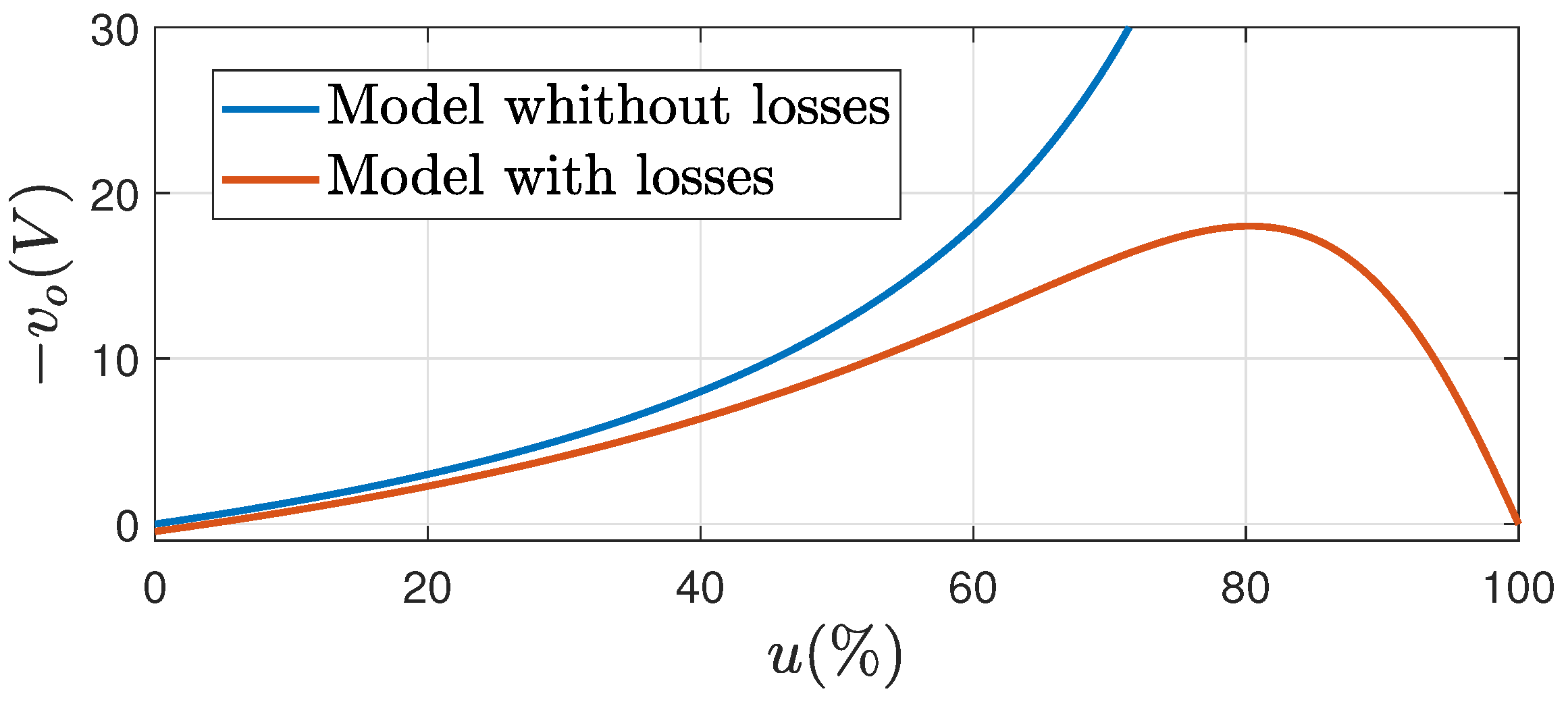
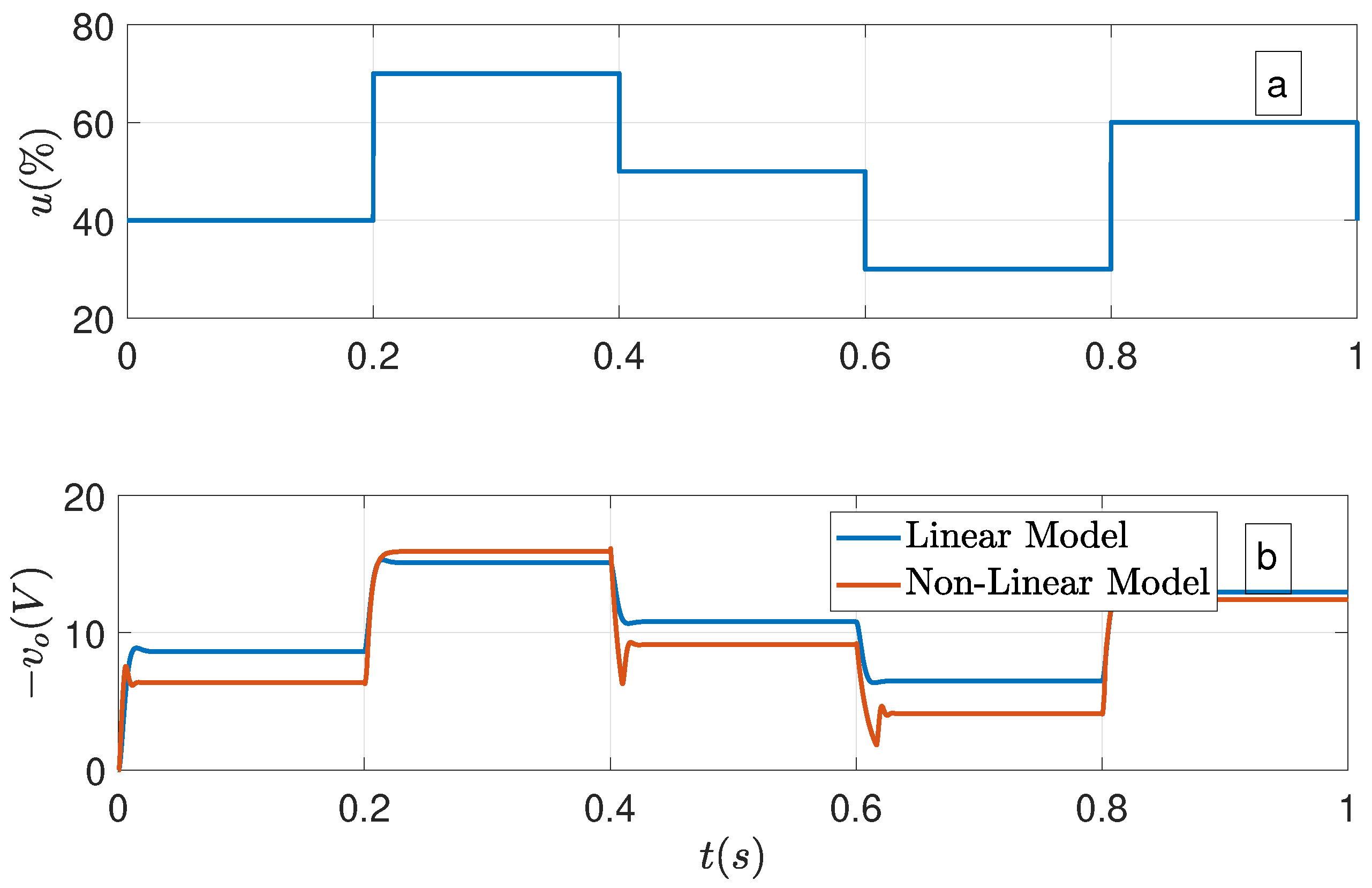
6.2. Analysis of the Ideal and Non-Ideal Models in Static-State Operation

The controllability of the power converter is related to the control signal values that can be applied as a duty ratio to the converter switcher. Therefore, the operational range of the electronic device is associated with the voltage values that the converter can give at its output. This range is restricted to the interval $[0,v_{max}]$.

The equilibrium points of the system are obtained based on the stationary state. The matrix Equation (34a) represents the equilibrium points associated with the ideal converter model [19]. The stationary state operation of the non-linear power converter corresponds to the matrix Equation (34b).

$$\left[\begin{array}{c}{\overline{i}}_L\\ \\ {\overline{v}}_C\end{array}\right]=\left[\begin{array}{c}\left(\frac{{\overline{v}}_C-E}{RE}\right){\overline{v}}_C\\ \\ -\left(\frac{\overline{u}}{1-\overline{u}}\right)E\end{array}\right]$$

(34a)

$$\left[\begin{array}{c}{\overline{i}}_L\\ \\ {\overline{v}}_C\end{array}\right]=\left[\begin{array}{c}\frac{\overline{u}(E+V_f)-V_f}{\overline{u}{r}_M+r_L+R{(1-\overline{u})}^2}\\ \\ -\frac{R(1-\overline{u})(\overline{u}(E+V_f)-V_f)}{\overline{u}{r}_M+r_L+R{(1-\overline{u})}^2}\end{array}\right]$$

(34b)

where ${\overline{i}}_L$, ${\overline{v}}_C$, and $\overline{u}$ are variables referring to the stationary state around a given operational point.

The performance of the ideal and non-ideal power converters at stationary state are compared in Figure 7. The common elements of both converters have identical characteristics. The test applies a 12 V tension at the converter input and a control signal sequence u restricted to the range $u\in \left[0;1\right]$.

The ideal converter provides an infinite voltage range, but this is impossible to achieve in real power converters due to electrical losses. These losses decrease the voltage and control input range. With a small duty ratio (0–40%), both converters have similar output voltages. However, as the duty ratio increases, the output voltage of the non-ideal converter differs significantly from the ideal.

The variation in the slope of the output voltage of the power converter must be considered for the design of the control scheme, mainly if it is based on continuous controllers. The controller cannot operate near this point because it can result in an undesirable behavior of the controlled converter. Due to the facts mentioned above, a duty cycle range of 0% to 80% is selected to ensure the stability of the controlled power converter. The selection of this range is justified because it provides better resolution for regulating the power converter. Any value outside this range is considered ineffective for the controller purpose.

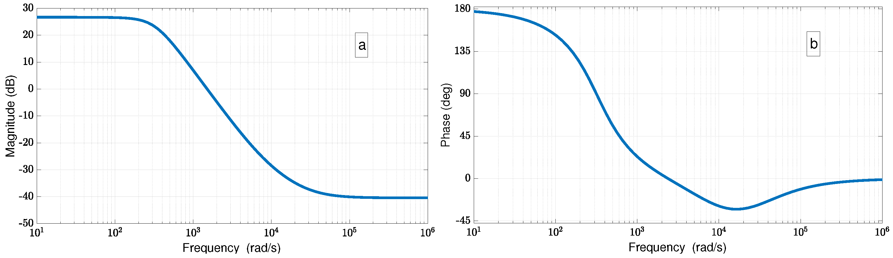
6.3. Identification of the Approximated Linear Model

The analysis related to the absolute and relative grade of the power converter is required for proposing a linear model structure that can generate a dynamical response similar to the one generated by the non-linear model. As can be seen in the state–space representation associated with the power converter model developed (see Equations (27)–(29) and (33)), the absolute grade of the converter is two, comprising the capacitor voltage $v_C$ and the power inductor current $i_L$. On the other hand, the relative grade of the system is zero because the output expression (see Equation (29)) depends explicitly on the control signal applied.

Another valuable criterion for constructing an approximated linear model from a nonlinear one is based on the analysis of the nonlinear model behavior around equilibrium points. The following matrix equations provide a state–space representation that describes the dynamics of a power converter operating at a specific operational point.

$$\dot{\mathbf{x}}=\mathbf{A}\mathbf{x}+\mathbf{B}u$$

(35)

$$y=\mathbf{C}\mathbf{x}+Du$$

(36)

where $\dot{\mathbf{x}}\in {\mathbb{R}}^n$ and $\mathbf{x}\in {\mathbb{R}}^n$. The term n is the number of states that characterize the system. In this case, the following change of notation is considered: $v_C=x_1$ and $i_L=x_2$, then $\mathbf{x}={\left[x_1{x}_2\right]}^T$.

The state matrix of the system ($\mathbf{A}$) and the input to state vector ($\mathbf{B}$) are generated by the following expressions:

$$\mathbf{A}={\left.\left[\begin{array}{cc}\frac{\partial F(\mathbf{x},u)}{\partial x_1}& \frac{\partial F(\mathbf{x},u)}{\partial x_2}\\ \\ \frac{\partial G(\mathbf{x},u)}{\partial x_2}& \frac{\partial G(\mathbf{x},u)}{\partial x_2}\end{array}\right]\right|}_{({\overline{x}}_1,{\overline{x}}_2,\overline{u})}$$

(37a)

$$\mathbf{B}={\left.\left[\begin{array}{c}\frac{F(\mathbf{x},u)}{\partial u}\\ \\ \frac{G(\mathbf{x},u)}{\partial u}\end{array}\right]\right|}_{({\overline{x}}_1,{\overline{x}}_2,\overline{u})}$$

(37b)

where $F(\mathbf{x},u)={\dot{x}}_1$ and $G(\mathbf{x},u)={\dot{x}}_2$. In our case, these functions can be rewritten as:

$$F(\mathbf{x},u)=-\frac{R}{C(R+r_c)}(1-u)x_2-\frac{1}{C(R+r_c)}{x}_1$$

(38a)

$$G(\mathbf{x},u)=\frac{1}{L_{eq}\left(x_2\right)}\left[-\left[u{r}_M+r_L+\frac{R{r}_C}{R+r_C}{(1-u)}^2\right]x_2+\frac{R}{R+r_C}(1-u)x_1+(E+V_f)u-V_f\right]$$

(38b)

The terms ${\overline{x}}_1$, ${\overline{x}}_2$, and $\overline{u}$ are the state variables and the control input applied at stationary state operation. The value of $L_{eq}\left(x_2\right)$ is given by the expression (33). The state-to-output vector ($\mathbf{C}$) and the feed-through term (D) are computed as follows:

$$\mathbf{C}={\left.\left[\begin{array}{cc}\frac{y(\mathbf{x},u)}{\partial x_1}& \frac{y(\mathbf{x},u)}{\partial x_2}\end{array}\right]\right|}_{({\overline{x}}_1,{\overline{x}}_2,\overline{u})}$$

(39a)

$$D={\left.\frac{y(\mathbf{x},u)}{\partial u}\right|}_{({\overline{x}}_1,{\overline{x}}_2,\overline{u})}$$

(39b)

where $y(\mathbf{x},u)=v_0$, so:

$$y(\mathbf{x},u)=\frac{R}{R+r_C}{x}_1-\frac{R{r}_C}{R+r_C}(1-u)x_2$$

(40)

The approximated linear model in its transfer function form can be obtained from the following equation:

$$G_a\left(s\right)=\mathbf{C}{(s\mathbf{I}-\mathbf{A})}^{-1}\mathbf{B}+D$$

(41)

The relations (34b), (37), (39) and (41) are used to generate the linear model of the system around an equilibrium point. The expression (42) is a linear structure of this power converter that models its dynamics around any equilibrium point.

$$G_a\left(s\right)=\frac{v_o\left(s\right)}{u\left(s\right)}=k\frac{(s+n_1)(s+n_2)}{(s+d_1)(s+d_2)}$$

(42)

where $d_1,d_2,n_1,n_2\in \mathbb{C}$. Also, as the power converter is stable when it operates in open loop, the real part of $d_1,d_2$ is less or equal than zero. The results related to the structure of the transfer function around a set of equilibrium points are shown in

Table 2. Transfer functions obtained from the linearization process.

u	k	${\mathit{n}}_1$	${\mathit{n}}_2$	${\mathit{d}}_1$	${\mathit{d}}_2$
0.2	8.8552 × 10${}^{-4}$	−3.2258 × 10${}^5$	4.1379 × 10${}^4$	−384.27 + 754.79i	−384.27 − 754.79i
0.4	8.8552 × 10${}^{-4}$	−1.1672 × 10${}^6$	1.0533 × 10${}^4$	−387.08 + 535.59i	−387.08 − 535.59i
0.5	8.8552 × 10${}^{-4}$	−2.0267 × 10${}^6$	5.5972 × 10${}^3$	−393.43 + 418.61i	−393.43 − 418.61i
0.6	8.8552 × 10${}^{-4}$	−3.4670 × 10${}^6$	3.1637 × 10${}^3$	−452.49 + 267.93i	−452.49 − 267.93i
0.8	8.8552 × 10${}^{-4}$	−1.0044 × 10${}^7$	113.1119	−3432.1	−163.8523

. These equilibrium points are selected inside the control signal range $u\in [0.2;0.8]$.

An essential characteristic of the approximated linear models in Table 2 is the non-minimum phase zero present in $\frac{v_o\left(s\right)}{u\left(s\right)}$. This behavior in a DC-DC buck–boost power converter has been reported in prior studies, such as [3,18,27]. This non-minimum phase zero restricts the operating frequencies of the converter, affecting its response time.

The recursive least-square identification algorithm with the forgetting factor is applied to identify a linear model. Analyzing the sampling time of the previously obtained results is necessary to apply the identification method. One criterion for determining the sampling time is based on the system time constant. However, this approach may not be practical in systems with oscillatory behavior. For detecting oscillations, the identification process requires a sampling time that is sufficiently small, satisfying the Nyquist/Shannon sampling period theorem, for their detection. In our study, since the equilibrium point analysis revealed a pair of complex conjugate poles, we selected the same sampling time of the simulation ($t_s={10}^{-4}$ s) because it is much shorter than the oscillation period of the system, which is approximately ${10}^{-2}$ s.

The discrete linear model, including the zero-order hold, has the following structure:

$$G_d\left(z\right)=\frac{v_o\left(z\right)}{u\left(z\right)}=\frac{n_2{z}^2+n_{1}z+n_0}{z^2+d_{1}z+d_0}$$

(43)

The vectors and matrix used along the identification procedure are structured as shown in the following relations:

$${\theta }_0=[0.1,0.1,0.1,0.1,0.1]$$

(44)

$$\varphi =\left[y\right(k-1),y(k-2),u(k),u(k-1),u(k-2\left)\right]$$

(45)

$$F=\left[\begin{array}{ccccc}100& 0& 0& 0& 0\\ 0& 200& 0& 0& 0\\ 0& 0& 300& 0& 0\\ 0& 0& 0& 400& 0\\ 0& 0& 0& 0& 400\end{array}\right]$$

(46)

vector (44) represents the initial values for the coefficients of the discrete model. The voltage input applied at the power input of the converter is $E=12$ V. The forgetting factor chosen for the procedure equals 0.95 for obtaining robustness in the identification performance. The input and output signals used for the identification process are shown in Figure 8a and Figure 8b, respectively. The identification process of the values for the discrete model coefficients is shown in Figure 8c; meanwhile, the estimation error along the whole procedure is represented in Figure 8d.

The mean of the error associated with the identification process is equal to 8.4193 × 10${}^{-4}$ V. As shown in Figure 8d, some error peaks represent the behavior of the algorithm to match the approximated model to the dynamics of the non-linear one.

Table 3. Data associated with the estimated parameters of the approximated linear discrete model.

Parameter	Mean	Variance	Corrected Value
$d_1$	−1.9473	0.0348	−1.9519
$d_0$	0.9487	0.0342	0.9529
$n_2$	0.0095	3.5856 × 10${}^{-4}$	0.0095
$n_1$	−0.0102	8.5356 × 10${}^{-5}$	−0.0106
$n_0$	−0.0193	8.5191 × 10${}^{-4}$	−0.0209

shows some static values of the estimated parameters. The data selected for generating the approximated linear model of the power converter are shown in the column called ”Corrected Value”. This quantity is set based on the value mean of the numeric estimation inside the variance previously computed of the data obtained.

The variance of the estimated values is always lower than its respective mean, as seen in Table 3. This result represents that the valid values of the estimated ones never change their sign, which is essential to guarantee a suitable identification procedure.

The discrete linear model estimated is related to the transfer function in the z-domain shown in the expression (47). This transfer function is structured considering a sampling time equivalent to ${10}^{-4}$ s.

$$G_d\left(z\right)=\frac{0.009499z^2-0.01056z-0.02086}{z^2-1.952z+0.9529}$$

(47)

This discrete model obtained in the s-domain is equivalent to the following continuous transfer function:

$$G_c\left(s\right)=\frac{0.009499s^2+199.6s-2.246\times {10}^6}{s^2+482.3s+1.04\times {10}^5}$$

(48)

The gain associated with the previous transfer function is 0.0095. This transfer function has two zeros: a minimum phase one $(z_1=-2.9128\times {10}^4)$ and a non-minimum phase one $(z_2=8.116\times {10}^3)$. The poles estimated by the identification algorithm are a pair of complex conjugated poles $(p_{1,2}=-241.16\pm 214.1i)$. The identification algorithm could detect the structure related to the converter dynamics analyzed. Figure 9 shows the response of both models (the linear and the non-linear one) when the same control input is applied to them. Both models shown in the Figure are strongly co-related.

The frequency response of the linear model estimated is shown in Figure 10. The initial value of the frequency response phase is 180${}^{\circ }$ because of the voltage inversion of this kind of converter at its output. The gain margin is −26.7 dB, and the phase margin is −169${}^{\circ }$, so this power converter is unstable in a closed-loop configuration.

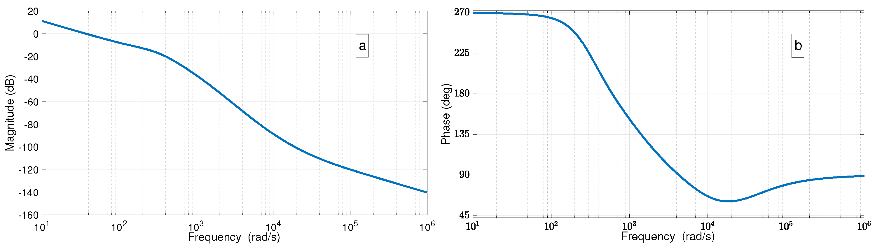
6.4. Controller Scheme Tuning

The voltage measured at the output of the power converter must be inverted to guarantee a good performance of the controller. In another way, if the reference voltage is positive, the controller can never follow that reference because of the inverting characteristic of this kind of power converter. Figure 11 shows the frequency response of the linear model controlled by a I controller coupled with a lead compensation action. The integral action is chosen to guarantee zero error at a stationary state. The gain associated with the controller is selected to reach an appropriate bandwidth, improving the response time. The lead compensation is commonly used for improving stability margins and achieves the desired result through the merits of its phase lead contribution [22]. The controller designed for regulating the linear model is equivalent to the transference function shown in (49).

$$C\left(s\right)=-10\frac{s+200}{s(s+1200)}$$

(49)

The phase and the gain margin of the power converter are 88.7${}^{\circ }$ and 26.9 dB, respectively. This phase margin guarantees robustness at variations over the equilibrium point. The bandwidth of this device is equal to 52.3 rad/s. If this bandwidth is not greater than the commutation time associated with the switcher, then it is valid for this converter. If the application for the power converter requires a wider bandwidth, the controller must be changed to guarantee good performance. The period of the lead compensation action is $T_{lead}=0.005$ s, and its alpha coefficient is $\alpha =\frac{1}{6}$.

Figure 12 shows the temporal responses of the controlled system considering both models (linear and nonlinear). The input voltage applied at the power input of the controller of the converter is 12 V.

As seen in Figure 12, the linear controller tuned has robustness to regulate the behavior of the non-linear model of the power converter using a tuning based on the frequency analysis of a linear approximated model. The proposed methodology is practical for designing linear controllers with outstanding performance.

The result related to the maximum voltage value that the non-ideal power converter can supply justifies the use of an anti-windup configuration to avoid the unstable behavior of the controlled device, when there is a higher reference value at the controller input. It is a maximum value on the saturation control signal of $u_{max}=80\%$. The anti-windup gain $\left(k_A\right)$ is defined using the following relation, and it is based on the results obtained from [17]:

$$k_A=5k_i=50.$$

(50)

Figure 13 shows the relevance of using the anti-windup scheme, which allows for the more robust behavior of the converter controller. This figure shows how the behavior of the converter is degraded by applying a reference voltage to the controller greater than a particular value.

7. Comparison of Results with Other Control Strategies

This section compares various control strategies employed in previous studies for regulating the DC-DC buck–boost power converter. The strategies for comparison include a non-linear PI controller tuned using Lyapunov functions [9] and an adaptive passivity control combined with a linear PI controller (adaptive PBC+PI) [13].

7.1. PBC Controller

The passivity control-based strategy PBC was used for regulating DC-DC power converters in many studies as [3,8,13,18,27]. The motivation for implementing it was related to its robustness when used on passive $SISO$ systems [28]. In [3], a structure of this control strategy was defined and used on an ideal DC-DC buck–boost power converter with a similar topology to the one considered in our study. The PBC proposed in [3] indirectly regulates the converter output voltage by the current of the power inductor. This regulation is considered in this way because of the non-minimum phase characteristic of the power converter. The following expression defines the indirect control law used for this controller:

$$i_d^{*}=v_d^{*}\left[\frac{v_d^{*}-E}{RE}\right]$$

(51)

where $i_d^{*}$ is the desired power inductor current, which depends on the desired voltage at the converter output. The expression (51) is obtained from the space representation of the ideal power converter model shown in the matrix Equation (34a). The PBC strategy is designed based on the mathematical model of the power device to be controlled [3]. For this reason, if the model does not consider some dynamical aspects or its parameters have some uncertainties, the PBC controller itself cannot guarantee the stationary zero error condition [18].

In [13], an adaptive controller that couples the PBC strategy with a classical PI controller was developed. The author defines this controller as Adaptive PBC+PI. The objective of PI inclusion was justified for avoiding errors in the operation on the stationary state. The expressions that define this control law are shown in the following equations:

$$\frac{d}{dt}{m}^c=\frac{1-\delta }{C\left[E-e_i{R}_1\right]}\left[{(1-\delta )}^2{i}_d^{*}-\frac{\delta E-e_i{R}_1}{R}-\frac{R_{1}C}{L}(\delta E+v_C(1-\delta ))\right]$$

(52)

where,

$$\delta =\mathsf{\Delta }+m^{c-1}$$

(53a)

$$\mathsf{\Delta }=k_p{e}_v+k_i\gamma$$

(53b)

$$\frac{d}{dt}\gamma =e_v$$

(53c)

$$e_i=i_d^{*}-i_L$$

(53d)

$\gamma$ is the voltage error derivative (see (53b) and (53c)); $\mathsf{\Delta }$ is the command signal generated by the classical PI added to the PBC strategy; $m^c$ is the control signal provided by the PBC+PI at the switcher converter; $m^{c-1}$ is the previous control signal generated; and $\delta$ is related to the values $m^{c-1}$ and $\mathsf{\Delta }$, and it is introduced into the Adaptive PBC+PI. The term $e_i$ is the difference between the desired and inductor currents. This control scheme allows the PBC to generate a signal based on the voltage error at the converter output. $R_1$ is the dissipative term that is integrated on the PBC strategy [19] and has to satisfy the condition $R_1>0$ to ensure the control system stability.

7.2. Non-Linear PI Controller

In [9], a non-linear PI controller is designed based on the Lyapunov function applied to the ideal converter mathematical model. The expressions that define the control law are as follows:

$$\varphi =k_p\left[{\mathsf{\Delta }}_1(E-v_d^{*})e_i+{\mathsf{\Delta }}_2{v}_d^{*}\left(\frac{v_d^{*}-E}{RE}{e}_v\right)\right]$$

(54a)

$$m=\frac{v_d^{*}}{v_d^{*}-E}+\varphi$$

(54b)

$$\frac{d}{dt}\xi =\gamma {\mathsf{\Delta }}_2\left(\frac{E}{v_d^{*}-E}+\varphi \right)e_v$$

(54c)

$$\gamma =\frac{{\mathsf{\Delta }}_1-{\mathsf{\Delta }}_2}{L{\mathsf{\Delta }}_1{\mathsf{\Delta }}_2}$$

(54d)

$$e_i=i_d^{*}+\xi -i_L$$

(54e)

$$e_v=v_d^{*}-v_o$$

(54f)

Equation (51) is used to calculate $i_d^{*}$. This controller has excellent robustness and high accuracy against variations in the applied source voltage and loads [9]. The required conditions to guarantee this performance are $k_p>0$, ${\mathsf{\Delta }}_1>0$ and ${\mathsf{\Delta }}_2>0$ [19].

7.3. Comparison of Results

The tuning of the adaptive PBC+PI and non-linear PI strategies is defined in [19] and is shown in

Table 4. Tuning parameters of the controllers.

Controller	Parameter	Value
Non-linear PI	$k_p$	0.1
	${\mathsf{\Delta }}_1$	0.2
	${\mathsf{\Delta }}_2$	0.1
Adaptive PBC+PI	$k_p$	0.01
	$k_i$	0.4
	$R_1$	2

.

7.3.1. Variations on Reference Voltage

Figure 14 displays the results of a tracking test for each control scheme. This test assesses the controlled converter ability to perform tracking tasks, which are relevant when the buck–boost converter is employed for regulating equipment, such as a DC motor, or as part of an MPPT controller in photovoltaic applications. The supplied voltage at the power input of the converter is set to 12 V. The sequence associated with the desired voltage and the converter voltage output is shown in Figure 14a. Figure 14b shows the power inductor current.

The PBC and the proposed controller are robust. However, the non-linear PI is not robust when the reference voltage is equal to or greater than a particular value, precisely when $v_d$ > 18 V. When the non-linear PI controller has stable performance, it produces a high and potentially dangerous current response in the inductor. So, this strategy demands components that are capable of handling higher current values than the other analyzed controllers. This increased demand for circuit elements leads to higher costs associated with the physical implementation of the converter.

When considering both robust control strategies under these operational conditions, the PBC controller exhibits a faster response than the proposed controller at the start of converter operations. When changing desired output voltages while the power converter is already operating in other operational conditions, the proposed controller demonstrates a slightly quicker response. The inductor current associated with the PBC controller is lower than that of the linear controller presented in this study. However, the difference between the two curves is not significantly relevant.

In this test, the controller with the best-reported performance was the PBC controller, even though its design does not consider the non-linear behavior associated with the power inductor. Also, the performance of the proposed linear controller is outstanding.

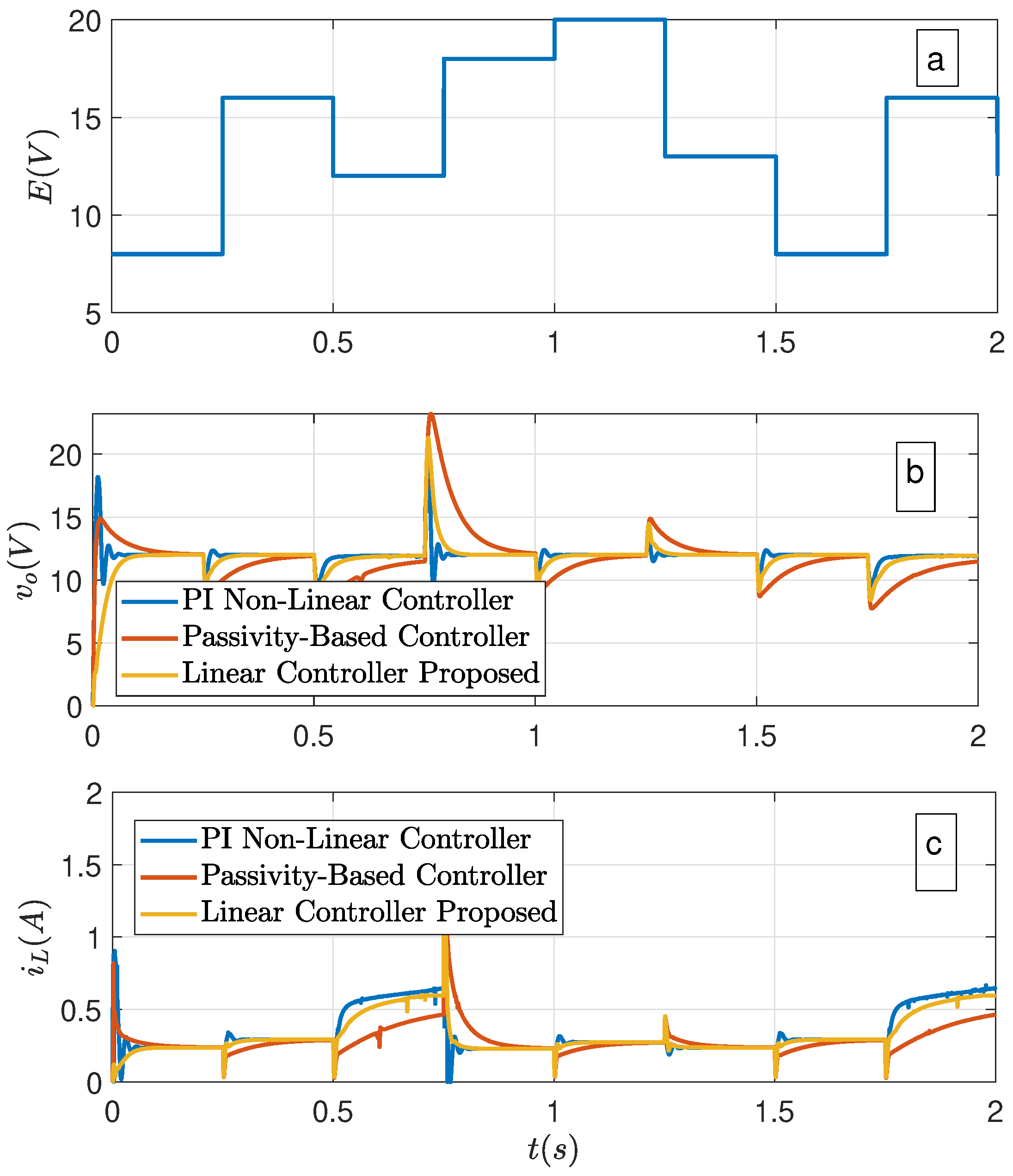
7.3.2. Variations on Supplied Voltage

Figure 15 displays how the analyzed controllers respond to voltage perturbations at the power converter input. This situation applies when the power converter maintains a constant output voltage to a particular load despite the variations at its input.

All three of the controllers exhibit stable behavior during this test. The non-linear PI controller generates the fastest response, and its inductor current peak values are considerably smaller than those obtained in the previous test. The PBC has the slowest response. Its response is characterized by over-damping behavior and results in the lowest current values in the power inductor. The response associated with the proposed controller is faster than the PBC controller and is over-damped. The current associated with the power inductor is less than the non-linear PI controller.

In this scenario, the PBC strategy is too slow to generate fast responses to reject these perturbations. Nevertheless, due to the low current values, components controlled by this strategy may be cost-effective. The non-linear PI controller stands out as the optimal choice as the response velocity is the primordial aspect. However, it is worth noting that the linear controller proposed in this study offers a response closely matching that of the non-linear PI controller.

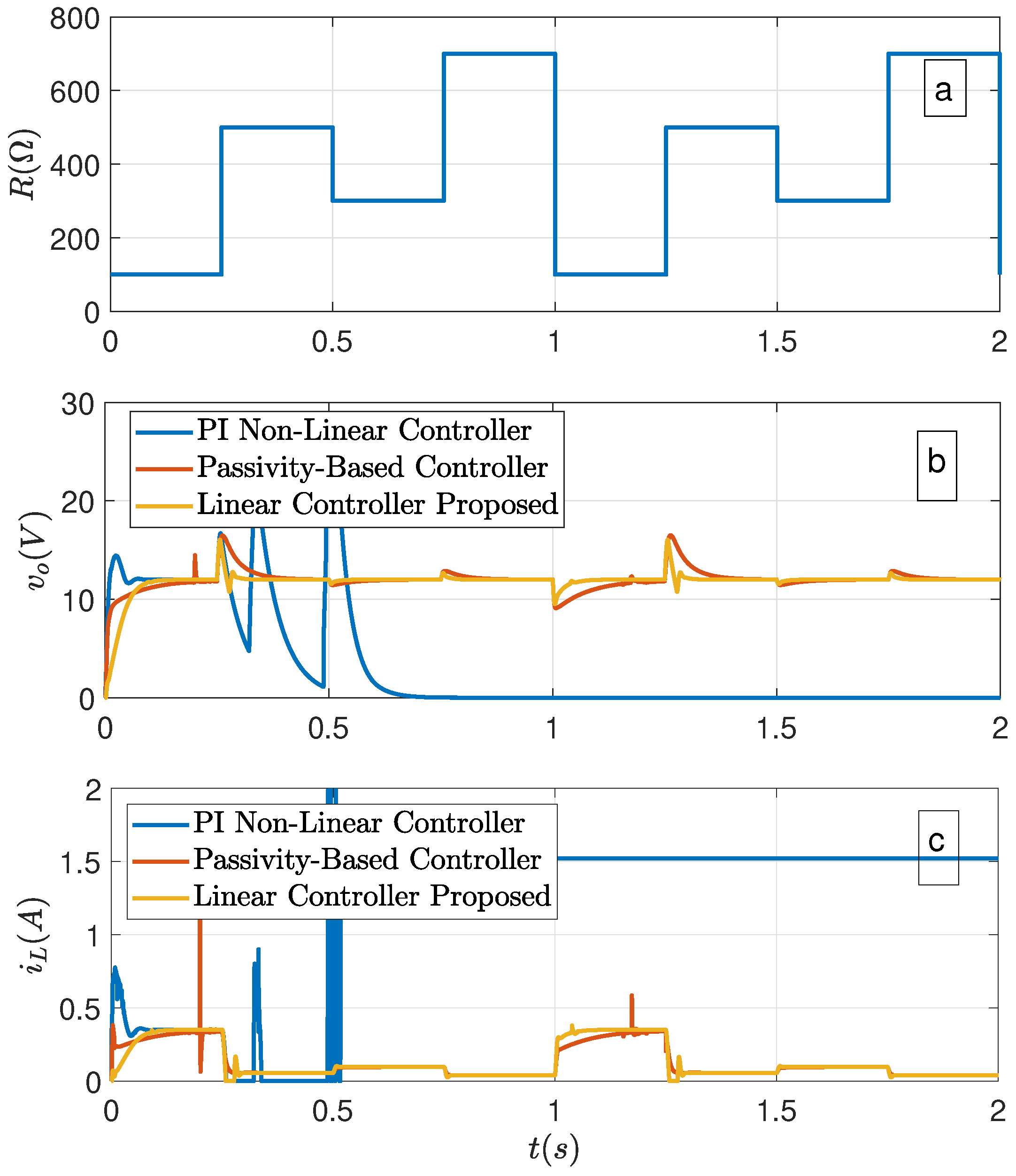
7.3.3. Variations on Load

Figure 16 illustrates the response of the controlled converter using the three previously analyzed strategies when variations in the connected load introduce perturbations.

In this scenario, the non-linear PI controller does not perform robustly. As shown in Figure 16, this controller cannot guarantee the desired output voltage in some cases. So, under these operational conditions, this controller is not appropriate.

The PBC strategy exhibited the slowest response, while the performance of the proposed linear controller is equally robust but faster in comparison. The inductor current requirements for the proposed controller and the PBC strategy are similar. Therefore, the proposed controller is well-suited for these operating conditions due to its robustness, fast response, and low inductor current combination.

7.4. Summary of the Results

Table 5. Summary of the results (◼—good performance), (◼—medium performance), and (◼—bad performance).

Controller		Test 1		Test 2		Test 3	Reference
Non-linear PI	◼	Not robust	◼	The fastest	◼	Not robust	[9]
Lyapunov-based				and robust
Passivity-based	◼	Robust	◼	The slowest	◼	Robust	[13]
		and fast		and robust		and slow
I + lead	◼	Robust	◼	Robust	◼	Robust	This article
compensation				and fast		and fast

shows a summary related to the results:

The proposed controller consistently outperformed all other options in the tests, displaying robustness and fast response times. This controller exhibits robust performance across various operating conditions, such as voltage reference changes and perturbations during the power converter operation.

However, the non-linear PI controller, when it generates stable behavior over the converter operation, delivers the fastest response. This control scheme has the drawback of demanding high inductor current values during transient operation, which requires higher-quality circuit elements, increasing manufacturing costs. The PBC strategy involves robust behavior but is unsuitable for applications requiring fast responses, particularly when the input voltage to the converter can change.

Another crucial factor to consider is the complexity of the controller structure and the number of required signals for implementing it. Both the PBC and non-linear PI controllers require output voltage and inductor current measurements, which can increase implementation complexity and associated expenses. Furthermore, the control laws applied in these controllers are more complex than the proposed control scheme, so they potentially require more computational effort than the proposed controller.

The controller proposed in this work relies on the output voltage of the power converter. Assuming that the controller is implemented as an analog device, it also requires control signal saturation limits, as depicted in Figure 3. If the controller is implemented as a digital device, it only requires the output voltage. Additionally, digital controller implementation can be more complex as data acquisition devices are often essential.

8. Conclusions

Using the Euler–Lagrange formalism, this study modeled a non-ideal DC-DC buck–boost power converter with electrical losses and a power inductor operating in its deep saturation region. The dynamical and stationary behavior of the power converter was analyzed. The results obtained from these analyses defined the restrictions on the operation of the power converter, such as its controllability.

The behavior of the power converter is regulated by a linear controller. The proposed tuning methodology identifies a linear model and analyzes the estimated model in the frequency domain. The identification procedure is based on the recursive least-square algorithm with the forgetting factor, which can effectively estimate a linear model based on the behavior of a non-linear model. The frequency analysis is based on the Bode diagram, a well-proven tool for knowing characteristics associated with the stability and robustness of the device controlled.

The controller designed and tested has an integral action, a lead compensation action, and an anti-windup scheme. The proposed controller performance was robust and had an excellent transient response and a simple structure. The performance of this linear controller is better than the other control strategies reviewed several operating conditions.

References

1. Wilamowski, B.M.; Irwin, J.D. Power Electronics and Motor Drives; CRC Press: Boca Raton, FL, USA, 2018. [Google Scholar]
2. Abdurraqeeb, A.M.; Al-Shamma’a, A.A.; Alkuhayli, A.; Noman, A.M.; Addoweesh, K.E. RST Digital Robust Control for DC/DC Buck Converter Feeding Constant Power Load. Mathematics 2022, 10, 1782. [Google Scholar] [CrossRef]
3. Ortega, R.; Perez, J.A.L.; Nicklasson, P.J.; Sira-Ramirez, H.J. Passivity-Based Control of Euler–Lagrange Systems: Mechanical, Electrical and Electromechanical Applications; Springer Science & Business Media: Berlin/Heidelberg, Germany, 2013. [Google Scholar]
4. Xie, L.; Shi, J.; Yao, J.; Wan, D. Research on the Period-Doubling Bifurcation of Fractional-Order DCM Buck–Boost Converter Based on Predictor-Corrector Algorithm. Mathematics 2022, 10, 1993. [Google Scholar] [CrossRef]
5. Riffo, S.; Gil-González, W.; Montoya, O.D.; Restrepo, C.; Muñoz, J. Adaptive Sensorless PI+Passivity-Based Control of a Boost Converter Supplying an Unknown CPL. Mathematics 2022, 10, 4321. [Google Scholar] [CrossRef]
6. Surya, S.; Williamson, S. Generalized Circuit Averaging Technique for Two-Switch PWM DC-DC Converters in CCM. Electronics 2021, 10, 392. [Google Scholar] [CrossRef]
7. Nam, N.N.; Kim, S.H. Robust Tracking Control of Dual-Active-Bridge DC-DC Converters with Parameter Uncertainties and Input Saturation. Mathematics 2022, 10, 4719. [Google Scholar] [CrossRef]
8. Sira-Ramirez, H.; Perez-Moreno, R.; Ortega, R.; Garcia-Esteban, M. Passivity-based controllers for the stabilization of Dc-to-Dc Power converters. Automatica 1997, 33, 499–513. [Google Scholar] [CrossRef]
9. Martinez-Lopez, M.J.; Moreno-Valenzuela, J.; He, W. A robust nonlinear PI-type controller for the DC–DC buck–boost power converter. ISA Trans. 2022, 129, 687–700. [Google Scholar] [CrossRef] [PubMed]
10. Oliveri, A.; Lodi, M.; Storace, M. Nonlinear models of power inductors: A survey. Int. J. Circuit Theory Appl. 2022, 50, 2–34. [Google Scholar] [CrossRef]
11. Kaiser, J.; Dürbaum, T. An Overview of Saturable Inductors: Applications to Power Supplies. IEEE Trans. Power Electron. 2021, 36, 10766–10775. [Google Scholar] [CrossRef]
12. Di Capua, G.; Femia, N. A Novel Method to Predict the Real Operation of Ferrite Inductors With Moderate Saturation in Switching Power Supply Applications. IEEE Trans. Power Electron. 2016, 31, 2456–2464. [Google Scholar] [CrossRef]
13. Wang, B.; Feng, H. The buck–boost converter adopting passivity-based adaptive control strategy and its application. In Proceedings of the 7th International Power Electronics and Motion Control Conference, Harbin, China, 2–5 June 2012; Volume 3, pp. 1877–1882. [Google Scholar] [CrossRef]
14. Lodi, M.; Oliveri, A.; Storace, M. Behavioral Models for Ferrite-Core Inductors in Switch-Mode DC-DC Power Supplies: A Survey. In Proceedings of the 2019 IEEE 5th International forum on Research and Technology for Society and Industry (RTSI), Florence, Italy, 9–12 September 2019; pp. 242–247. [Google Scholar] [CrossRef]
15. Almawlawe, M.D.; Kovandzic, M. A Modified Method for Tuning PID Controller for buck–boost Converter. Int. J. Adv. Eng. Res. Sci. 2016, 3, 236938. [Google Scholar] [CrossRef]
16. Vijayalakshmi, S.; Arthika, E.; Priya, G.S. Modeling and simulation of interleaved buck–boost converter with PID controller. In Proceedings of the 2015 IEEE 9th International Conference on Intelligent Systems and Control (ISCO), Coimbatore, India, 9–10 January 2015; pp. 1–6. [Google Scholar] [CrossRef]
17. Sanchez-Flores, J.A.; Gonzalez-Valdes, J.Y.; Liceaga-Castro, J.U.; Liceaga-Castro, E.; Amezquita-Brooks, L.A.; Garcia-Salazar, O.; Martinez-Vazquez, D.L. Experimental workbench for aircraft ram air micro-turbine generators. In Proceedings of the 2017 IEEE International Autumn Meeting on Power, Electronics and Computing (ROPEC), Ixtapa, Mexico, 8–10 November 2017; pp. 1–6. [Google Scholar] [CrossRef]
18. Wang, B.; Ma, Y. Research on the passivity-based control strategy of buck–boost converters with a wide input power supply range. In Proceedings of the 2nd International Symposium on Power Electronics for Distributed Generation Systems, Hefei, China, 16–18 June 2010; pp. 304–308. [Google Scholar] [CrossRef]
19. Martinez-Lopez, M.J. Modelado y Control de Convertidores de Potencia; Tesis de grado, Instituto Politécnico Nacional: Mexico City, Mexico, 2021. [Google Scholar]
20. Huba, M.; Chamraz, S.; Bistak, P.; Vrancic, D. Making the PI and PID Controller Tuning Inspired by Ziegler and Nichols Precise and Reliable. Sensors 2021, 21, 6157. [Google Scholar] [CrossRef] [PubMed]
21. Zand, J.P.; Sabouri, J.; Katebi, J.; Nouri, M. A new time-domain robust anti-windup PID control scheme for vibration suppression of building structure. Eng. Struct. 2021, 244, 112819. [Google Scholar] [CrossRef]
22. Ogata, K. Modern Control Engineering; Prentice Hall: Upper Saddle River, NJ, USA, 2010; Volume 5. [Google Scholar]
23. Liceaga-Castro, J.U.; Siller-Alcalá, I.I.; Alcántara-Ramírez, R. least-square Identification using Noise Reduction Disturbance Observer. Trans. Syst 2019, 18, 313–318. [Google Scholar]
24. Jiménez-González, J. Identificación de Parámetros en Tiempo real de un Motor de CD de Imanes Permanentes sin Escobillas. Master’s Thesis, Universidad Autónoma Metropolitana (México), Unidad Azcapotzalco, Azcapotzalco, Mexico, 2021. [Google Scholar]
25. Jimenez-Gonzalez, J.; Gonzalez-Montañez, F.; Jimenez-Mondragon, V.M.; Liceaga-Castro, J.U.; Escarela-Perez, R.; Olivares-Galvan, J.C. Parameter Identification of BLDC Motor Using Electromechanical Tests and Recursive Least-Squares Algorithm: Experimental Validation. Actuators 2021, 10, 143. [Google Scholar] [CrossRef]
26. Landau, I.D.; Zito, G. Digital Control Systems: Design, Identification and Implementation; Springer: Berlin/Heidelberg, Germany, 2006; Volume 130. [Google Scholar]
27. Sira-Ramirez, H.J.; Silva-Ortigoza, R. Control Design Techniques in Power Electronics Devices; Springer Science & Business Media: Berlin/Heidelberg, Germany, 2006. [Google Scholar]
28. Liceaga-Castro, J.U.; Siller-Alcalá, I.I.; Liceaga-Castro, E.; Amézquita-Brooks, L.A. MIMO Passive Control Systems Are Not Necessarily Robust. J. Control Sci. Eng. 2016, 2015, 508102. [Google Scholar] [CrossRef]
Figure 1. DC-DC buck–boost converter topologies analyzed. (a) Ideal and (b) non-ideal considering electrical losses and the non-linear inductor.
Mathematics 11 04617 g001
Figure 2. Equivalent circuits for modeling an ideal DC-DC buck–boost converter. (a) Circuit when the control signal is at high level ( u = 1 ) . (b) Converter equivalent circuit when the control signal is at low level ( u = 0 ) .
Mathematics 11 04617 g002
Figure 3. Scheme of the proposed controller.
Mathematics 11 04617 g003
Figure 4. Proposed methodology to design the controller.
Mathematics 11 04617 g004
Figure 5. Equivalent circuits of the converter operation state. (a) On ( u = 1 ) . (b) Off ( u = 0 ) .
Mathematics 11 04617 g005
Figure 6. Behavior of the non-linear inductance.
Mathematics 11 04617 g006
Figure 7. Comparison between the ideal and non-ideal power converter models.
Mathematics 11 04617 g007
Figure 8. Identification process. (a) Input signal applied to the power converter model. (b) Output signal generated. (c) Estimation of the parameters of the discrete linear model. (d) Error associated with the estimation of the parameters.
Mathematics 11 04617 g008
Figure 9. Comparison of the linear and the non-linear models. (a) Input voltage applied at the control input. (b) Output voltage.
Mathematics 11 04617 g009
Figure 10. Bode diagram related to the approximated linear model of the power converter. (a) Magnitude. (b) Phase.
Mathematics 11 04617 g010
Figure 11. Bode diagram related to the approximated linear model of the I-controller. (a) Magnitude. (b) Phase.
Mathematics 11 04617 g011
Figure 12. Temporal response of the controlled systems.
Mathematics 11 04617 g012
Figure 13. Differences between the anti-windup built-in controller and the linear controller during the regulation of the power converter operation.
Mathematics 11 04617 g013
Figure 14. Comparison of the response generated by the controllers under changes in the reference voltage. (a) Output voltage. (b) Inductor current.
Mathematics 11 04617 g014
Figure 15. Comparison of the response generated by the controllers reviewed above and the proposed one when changes in the supplied voltage are applied. (a) Input voltage applied. (b) Behavior of the output voltage and (c) inductor current.
Mathematics 11 04617 g015
Figure 16. Comparison of the response generated by the controllers under changes in the connected load. (a) Load connected at the converter output. (b) Output voltage. (c) Inductor current.
Mathematics 11 04617 g016