Abstract
Long COVID, a long-lasting disorder following an acute infection of COVID-19, represents a significant public health burden at present. In this paper, we propose a new mechanistic model based on differential equations to investigate the population dynamics of long COVID. By connecting long COVID with acute infection at the population level, our modeling framework emphasizes the interplay between COVID-19 transmission, vaccination, and long COVID dynamics. We conducted a detailed mathematical analysis of the model. We also validated the model using numerical simulation with real data from the US state of Tennessee and the UK.
MSC:
92D30
1. Introduction
A serious consequence following infection with SARS-CoV-2 is the potential occurrence of a long-lasting disorder known as post-acute sequelae of COVID-19 (or, long COVID) [1,2]. The cause of long COVID is unclear at present, but possible contributors include persistent reservoirs of SARS-CoV-2 in certain tissues and their continued interactions with host microbiome communities, injuries to one or more organs from the acute infection, ongoing activities of primed immune cells and other immune dysregulations, clotting/coagulation issues, and dysfunctional vagus nerve signals [3,4,5].
A number of studies have highlighted the persistence and complications of the long COVID syndrome. For example, a cohort study followed 147 Italian patients who were hospitalized for COVID-19 and found that 87% still had symptoms 60 days after they were discharged from the hospital [6]. Another study [7] found that 76% of hospitalized COVID-19 patients (or, 1265 out of 1655) in Wuhan, China, were still experiencing symptoms 6 months after their infection. In the United States, CDC estimated that up to a third of COVID-19 cases may result in long-term symptoms [8], indicating that tens of millions of Americans diagnosed with COVID-19 may endure long-lasting consequences of the illness. The situation is further complicated by the fact that individuals who are infected with only mild symptoms, and those who are fully vaccinated but later develop breakthrough infections, can become COVID long-haulers [9,10,11].
In order to assess the impact of long COVID on the healthcare system and to design effective strategies for resource distribution, it is critical to quantify and predict the burden of long COVID at the population level. However, several systematic reviews and meta-analyses found that COVID long-haulers exhibited a wide variety of symptoms and that the long COVID rates are highly heterogeneous across different populations, ranging from 10% to 67% [11,12,13,14,15]. Such a heterogeneous pattern indicates that no single formula can be applied to every population to quantify the burden of long COVID. Instead, the evaluation and prediction of long COVID prevalence have to take into account the specific population characteristics and the epidemic/pandemic trends.
Mathematical models can overcome such challenges and help us to better quantify the population dynamics associated with long COVID. However, in contrast to the large number of mathematical, statistical, and computational models already published for COVID-19 transmission and spread (see reviews in [16,17,18,19]), very few modeling studies have been devoted to long COVID. The currently available models for long COVID are mainly based on machine learning and statistical techniques, with a focus on identifying individuals at risk of long COVID [20,21,22,23,24,25]. Their findings, though very useful, do not improve the understanding of the population dynamics of long COVID. Moreover, none of these studies have employed mechanistic models.
In this work, we propose a novel mechanistic model based on differential equations to investigate the dynamics of long COVID and its population-level prevalence. Since long COVID stems from acute infection, we will link the population dynamics of long COVID with the transmission dynamics of COVID-19. In addition, since COVID-19 vaccines have played an important role in fighting the virus, we will also incorporate the impact of vaccination in our model. Our goal is to accurately predict the prevalence of long COVID in a given population with the available data. We will implement the model in real-world applications using data from both the US and the UK.
The remainder of this paper is organized as follows. We present the formulation of our mechanistic model in Section 2 and perform a detailed mathematical analysis in Section 3. We then present data fitting and numerical simulation in Section 4. Finally, we conclude our paper with some discussion in Section 5.
2. Model Formulation
We used differential equations to construct our mathematical model and investigated the population dynamics of long COVID. We considered a model that involves five compartments representing the number of the following individuals: the susceptible individuals (denoted by S), the vaccinated individuals (denoted by V), the infected and infectious individuals with short-term symptoms (denoted by I), the individuals with long-term symptoms; i.e., COVID long-haulers (denoted by L), and the recovered individuals (denoted by R). Based on numerous clinical studies, the duration of infectiousness of SARS-CoV-2 is always limited to a relatively short period [26]. We, thus, assume that individuals with long COVID are not contagious.
The model is described by the following differential equations:
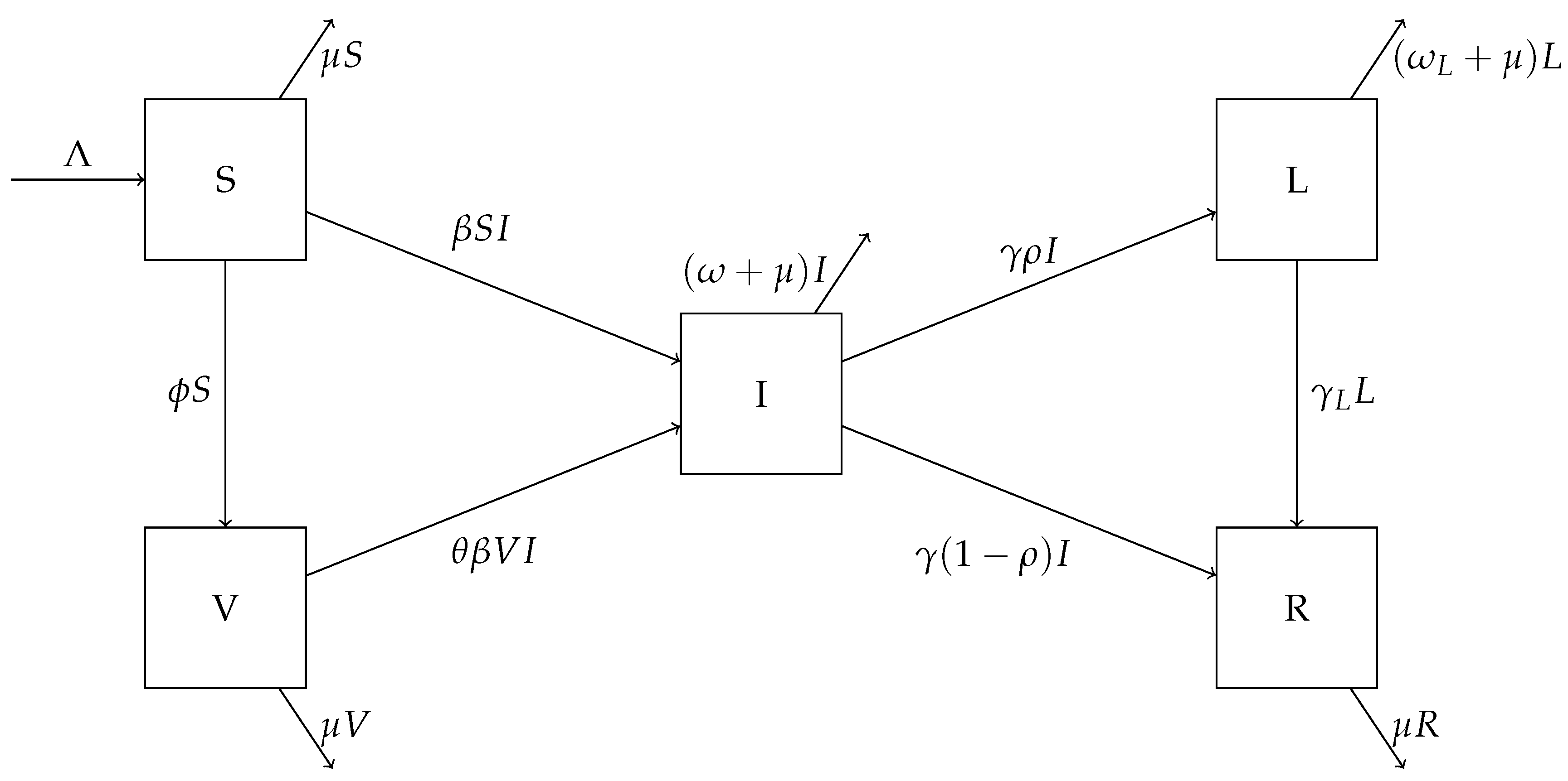
A flow chart for this model is shown in Figure 1. The parameter is the population influx rate, is the transmission rate, is the natural death rate for the human hosts, and is the vaccination rate. Susceptible individuals become infected by contacting infectious individuals. In addition, susceptible individuals are vaccinated at the rate . We assume that a portion of () in vaccinated individuals are at risk for breakthrough infections, that is, the degree of protection for the vaccines is . Infected individuals exit the acute infection period at the rate ; among these, a portion will develop long COVID and enter the L compartment, whereas the other portion will truly recover from the disease and enter the R compartment. Since we are concerned with a relatively long time period, individuals in all these compartments are subject to natural mortality at an average rate . In addition, the parameter is the rate of recovery for COVID long-haulers, and and are the disease-induced death rates in the acute infection and long COVID states, respectively.
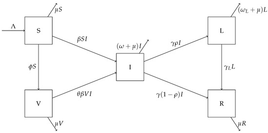
Figure 1.
A flow chart showing movement between the compartments of the system (1).
3. Mathematical Analysis
System (1) has a feasible domain
It can be easily verified that is positively invariant for the vector field of (1). It is also straightforward to obtain the following result:
Theorem 1.
System (1) has a unique disease-free equilibrium (DFE) in the domain Ω
The basic reproduction number of our model can be derived by the standard next-generation matrix technique [27], with the new infection matrix F and the transition matrix V computed as
The spectral radius of the next-generation matrix then gives the basic reproduction number of system (1):
Note that the term related to in Equation (4) represents the risk associated with the breakthrough infection.
Theorem 2.
System (1) has a positive endemic equilibrium
in Ω if and only if . The endemic equilibrium is unique when it exists.
Proof.
At a nontrivial equilibrium of system (1), we have
Now, we write each equation as a function of I. From (6)–(8), we obtain
and
respectively. Substituting (11) into (12), we obtain
Similarly, substitution of (11) into (13) yields
Equating (14) and (15), we obtain an equation in terms of a single variable I:
where the function f is defined as
The function is strictly decreasing for , and when . Hence, Equation (16) has a positive solution at if and only if
Through simple algebraic manipulation, it can be easily seen that Equation (18) is equivalent to . Clearly, the positive solution is unique when , due to the monotonicity of the function f.
Consequently, S, V, L, and R at the positive equilibrium can all be uniquely determined from based on the equations presented above, and this positive equilibrium clearly belongs to . Hence, there is a unique endemic equilibrium for system (1) if and only if . □
From [27], we know that the DFE is locally asymptotically stable when and unstable when . The result below establishes the local stability for the endemic equilibrium.
Theorem 3.
When , the endemic equilibrium is locally asymptotically stable.
We provide the proof of Theorem 3 in Appendix A. In what follows, we focus on the global stability properties of the DFE and the endemic equilibrium.
Theorem 4.
When , the DFE is globally asymptotically stable in Ω. When , the endemic equilibrium is globally asymptotically stable in Ω.
Proof.
We first consider the case , where the endemic equilibrium exists and is unique. We aim to establish that all the orbits of approach . To that end, we introduce the following Lyapunov function [28]:
Taking the derivative of along the solution of system (1) gives us
where the dot notation is used for the time derivatives of S, V, and I. We will show that . To do so, we will manipulate the three parts in Equation (20) separately. For convenience, we will denote these terms by (21)–(23). Our first term is equal to
Similarly, the second term in (20) is
Now, the last term of (20) is
From here, we will begin the process of canceling out many terms and showing that all that remains are nonpositive terms. We can rewrite the following terms as
from (8). Therefore,
Similarly, from (7), the terms in (22) can be rewritten as
giving us
Note that, in all of the terms of (21)–(23), there are common factors of We will simplify by first summing all of the terms from (21)–(23) that share one of these common factors before combining what we have left afterwards. Starting with
Many terms can immediately be canceled. Doing so gives
For terms that share a common factor of ,
This leaves us with one remaining term with a common factor of :
Now, by combining all of the three terms, we are left with
all of which are nonpositive terms since the arithmetic mean is greater than or equal to the geometric mean. Hence, and the equality holds if and only if , which shows that for all the solution orbits. Consequently, letting , we immediately obtain and from the last two equations of system (1). This establishes the global asymptotic stability of the endemic equilibrium when .
When , the DFE is the only equilibrium of system (1). We consider the Lyapunov function
which yields
along the solution of system (1). It can be easily observed that the algebraic manipulations we performed previously for will still hold for and all the terms associated with will disappear. We thus obtain
With similar arguments as before, we can establish the global asymptotic stability of the DFE when . □
These theoretical results concerning the different types of equilibria and their stability properties, with a sharp threshold at , are common in many epidemiological models [27,29]. Nevertheless, an important message from Theorems 2–4 is that long COVID may persist in the host population in the long run, unless COVID-19 is completely eradicated. In the next section, we will utilize a numerical simulation to implement our model for real-world applications. We fitted and simulated the model using reported data from relatively short time periods to gain insights for the population-level progression of long COVID.
4. Numerical Simulation
We conducted numerical simulation with real data to validate our model. In contrast to the large amount of surveillance data for COVID-19, time series data for long COVID at the population level are very rare at present. We performed two simulation studies. The first one was for the state of Tennessee in the US, where detailed data for COVID-19 cases, deaths, and vaccination coverage are available [30], but there are no population-level data available for long COVID. The second study was concerned with the UK which, as an exception, published monthly data for long COVID prevalence in the UK population through its Office for National Statistics (ONS) [31].
4.1. Simulation for the Tennessee State in the US
We first applied our model to the COVID-19 data for the US state of Tennessee for the 4-month period between 31 August 2021 and 30 December 2021. An estimation given by the US Census Bureau of the total population in Tennessee on 1 July 2021 gave us a value of 6,975,218 [32]. Our time period was relatively short, so we assumed that immigration and emigration were equal, and that the natural birth rate was equal to the natural death rate, . We defined the natural death rate as the inverse of the life expectancy, which in 2019, before COVID-19 started in Tennessee, was 75.6 years [33]. We were then able to define the population influx rate as the product of the natural birth rate and the total population: . We defined as the recovery rate for acute infections, calculated as the reciprocal of the acute infection period reported in [34]. For , i.e., the disease-induced death rate for acute infections, we used the estimate provided in [35]. The breakthrough infection ratio, , ranged from to in the US [36], and we took an average in this study. The values for these parameters can be found in Table 1.

Table 1.
Parameter values for the simulation of the Tennessee data.
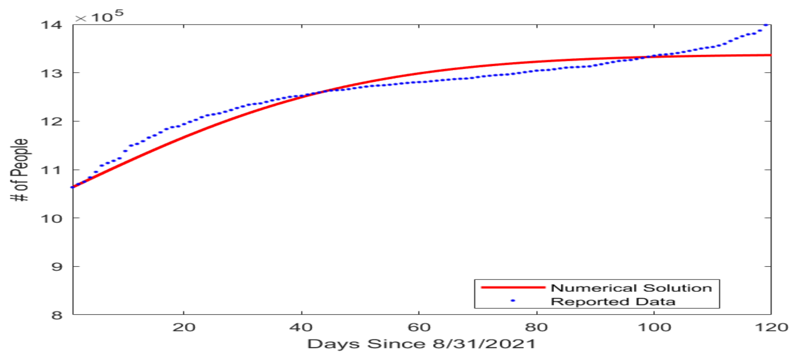
In our model, the susceptible, vaccinated, and infected compartments form a system that is not dependent on long COVID cases or the recovered compartment. So next, we estimated the transmission rate and the vaccination rate by fitting a simplified model consisting of only the S, V, and I compartments to the COVID-19 infection and vaccination data reported on a daily basis by the Tennessee Department of Health [30]. The initial condition for this simulation was set as (, , ) = , based on the reported data for the number of fully vaccinated individuals and infected individuals in Tennessee on 31 August 2021. The fitted parameter values are given in Table 2 and the result of the data fitting for the number of cumulative cases is shown graphically in Figure 2.

Table 2.
Parameter estimates found by fitting the Tennessee data.
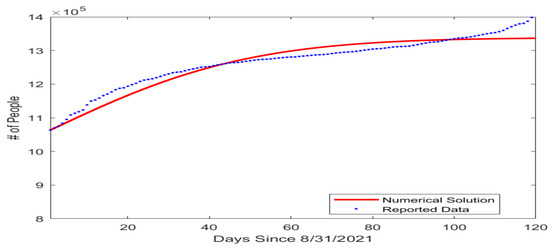
Figure 2.
Fitting result for the number of cumulative COVID-19 cases in the US state of Tennessee beginning from 31 August 2021. The horizontal axis represents the number of days since 31 August 2021, and the vertical axis represents the number of cumulative cases.
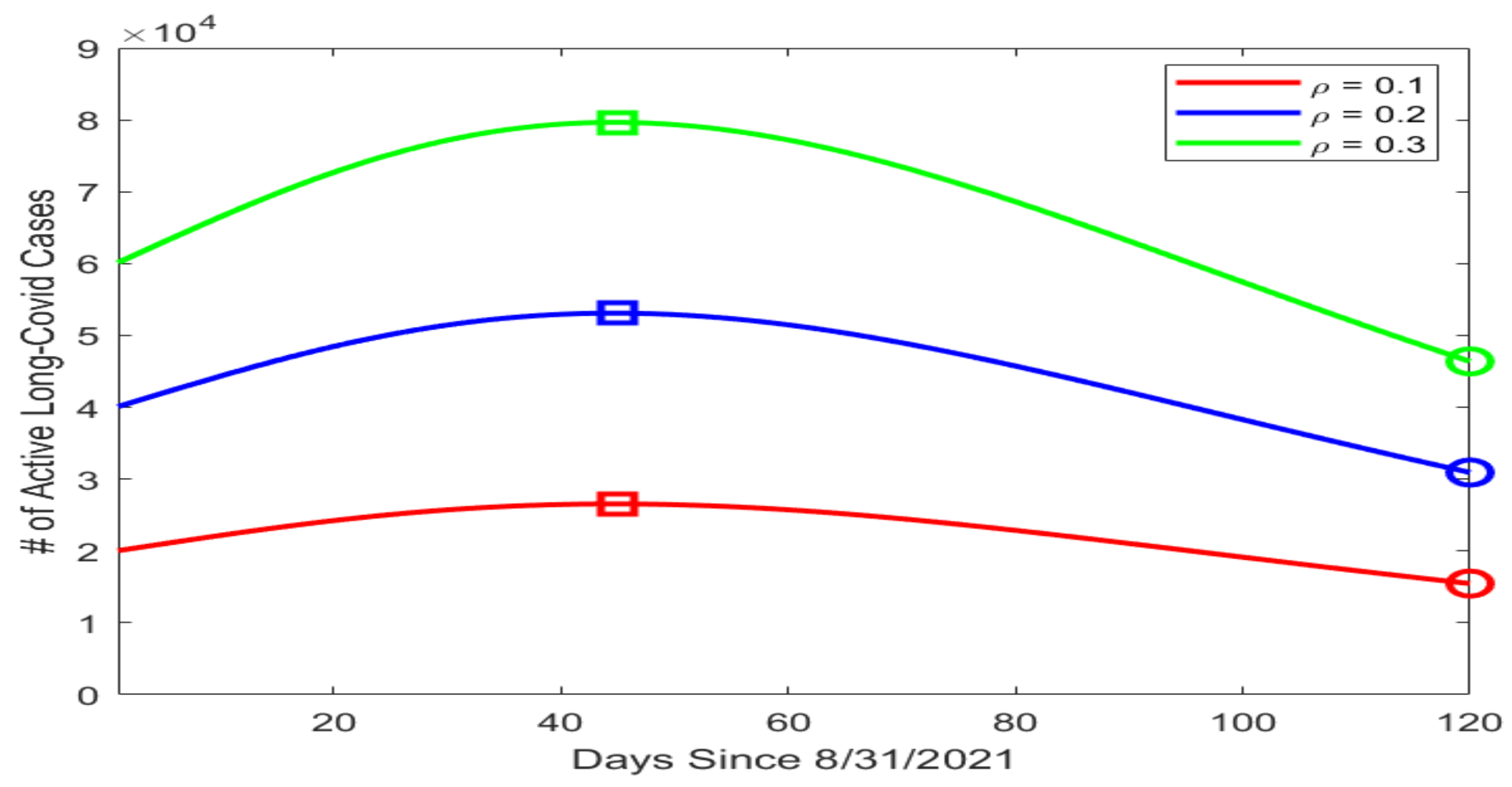
Based on our data fitting results, which included the number of active infections I in particular, we proceeded to conduct a numerical simulation for the possible prevalence levels of long COVID in Tennessee using the equation for the L compartment in system (1). We assumed that the mortality rate caused by long COVID was much lower than that caused by the acute infection, with , and that the average recovery period for long COVID was 90 days, with per day. We then picked three different values for , i.e., the portion of infected individuals who went on to develop long COVID, with , , and . Figure 3 displays the simulation curves for the number of active long COVID cases with the three values of . The highest and lowest points on each curve are marked by a square and a circle, respectively. We observed that the peak of L ranged from about (when ) to almost (when ). Even with the minimal estimate of , the lowest point on the simulation curve was , indicating a substantial public health burden caused by long COVID.
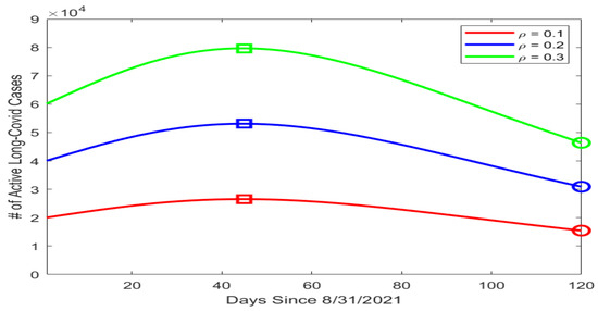
Figure 3.
Simulation results for the number of active long COVID cases in Tennessee using different values of . The horizontal axis represents the number of days since 31 August 2021, and the vertical axis represents the number of active long COVID cases. On each simulation curve, the square marks the peak and the circle marks the lowest point of the curve.
Because long COVID data are not available for the Tennessee population, we were not able to fit the parameters relevant to long COVID dynamics and predict the progression of long COVID in Tennessee. Nevertheless, our simulation results provide possible ranges for the prevalence of long COVID in this population, which could inform the public health administration in their design of control and intervention strategies.
4.2. Simulation for the UK
In addition to the regular, daily reported data for COVID-19 infections, the UK Office for National Statistics (ONS) has published survey data for the prevalence of long COVID in the UK population on a monthly basis [31]. The time period covered by the long COVID data starts from 6 February 2021. The ONS data allowed us to fit our model to the number of long COVID cases. We focused our attention on fitting the L compartment in system (1), where the variable I involved in the L equation was determined by the reported number of active COVID-19 cases. We set the time from 6 February 2021 to 4 July 2022, a period about 17 months, for model fitting, and the time from 5 July 2022 to 6 December 2022, a period about 5 months, for model testing.
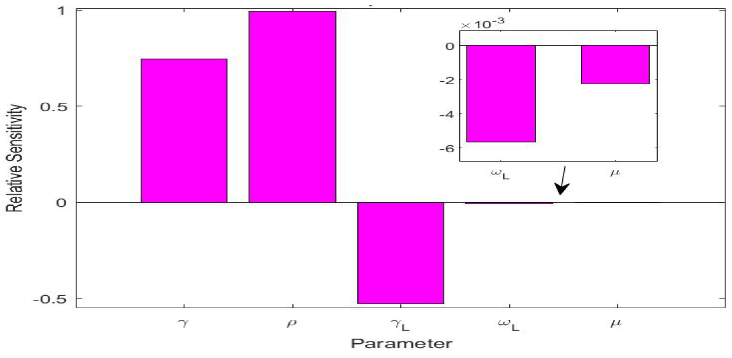
The values of the parameters for the UK simulation study are listed in Table 3. There were five parameters, i.e., , , , , and , that were involved in the L equation in system (1). We also conducted a sensitivity analysis for these five parameters in terms of the variable L, using the method from [37] for computing relative sensitivities. The results are presented in Figure 4. We observed that , , and were the three most sensitive parameters, while and had very low sensitivities. This indicates that and would have very little impact on the long COVID prevalence L. We calculated the natural death rate from the demographic information of the UK population [38]. We took the long COVID-induced death rate per day, i.e., the same value used in the Tennessee simulation. We additionally noted that the recovery rate was determined by the characteristics of the acute infection. We thus set the (average) recovery period from the acute infection as days, based on reported values for COVID-19 in the UK [39].

Table 3.
Parameter values for the simulation of the UK long COVID data.

Figure 4.
Relative sensitivities for the five parameters , , , , and that are related to the long COVID compartment L.
We proceeded to use data fitting to estimate the two key parameters and associated with the long COVID prevalence. Specifically, we fitted the L equation in our model to the monthly reported long COVID data over the 17-month fitting period. Next, we conducted a numerical simulation to generate a prediction for the 5-month testing period using the parameter values estimated from the fitting period.
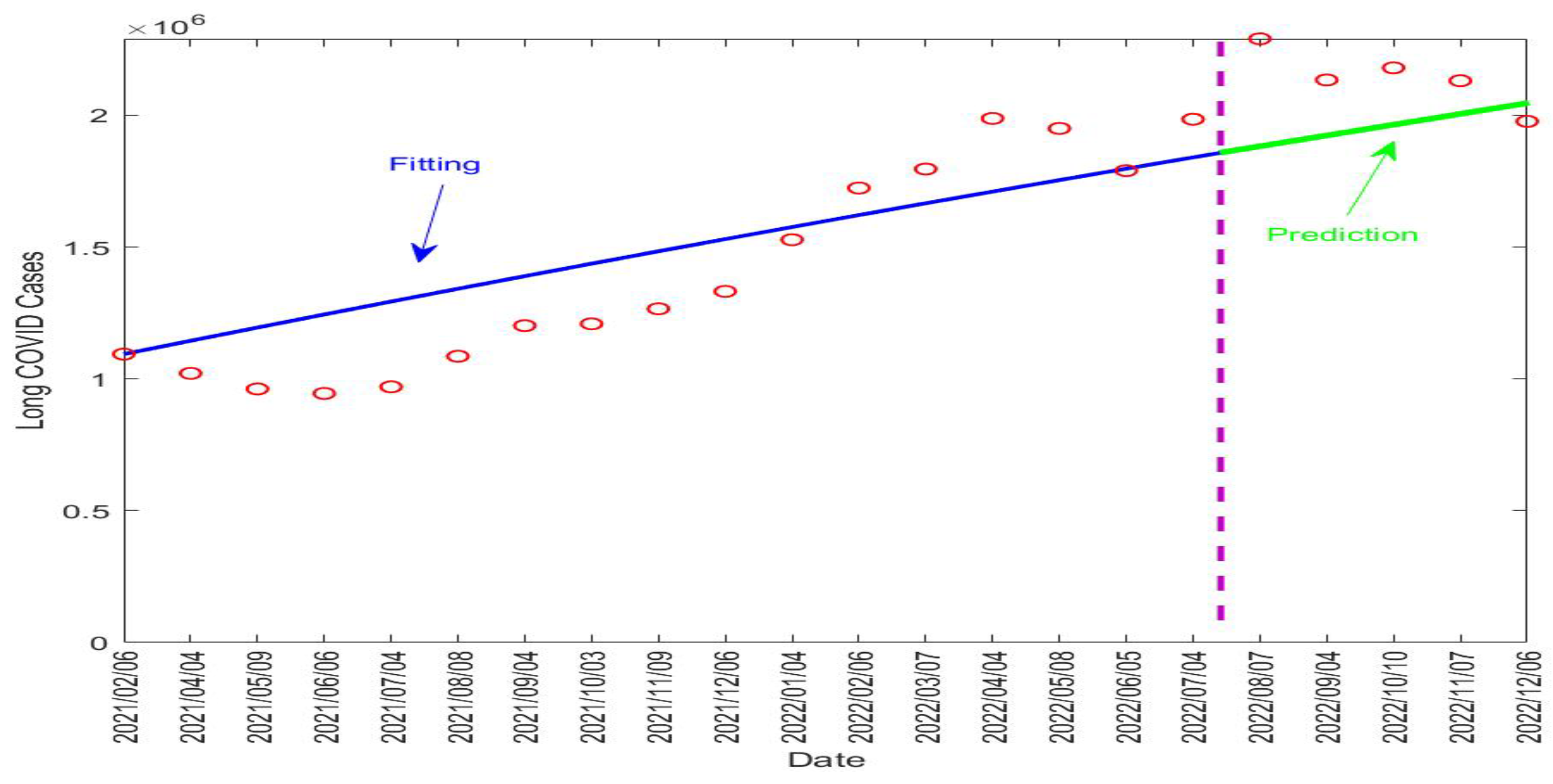
Table 4 lists the fitted parameter values. Figure 5 displays the fitting and prediction curves for the number of active long COVID cases in the UK, compared with the ONS data. The vertical dashed line in the figure separates the fitting and prediction periods.

Table 4.
Parameter estimates found by fitting the UK long COVID data.

Figure 5.
Fitting and prediction results for the long COVID cases in the UK from 6 February 2021 to 6 December 2022. The vertical dashed line in purple separates the fitting and prediction periods. The red circles represent the reported data. The blue solid line represents the fitting result and the green solid line represents the prediction result.
Our fitting result for shows that about 31.6% of the infected individuals in the UK went on to develop long COVID. The fitted value for the recovery rate of long COVID was per day, indicating that long COVID would last about days on average in the UK population. This is indeed very close to the assumed value of 90 days in our simulation study for the Tennessee data. These numbers, together with the predictive capability of the model, can provide useful quantitative information to assess the burden of long COVID in the UK and to guide relevant policy developments and resource allocation.
5. Discussion
As stated in a recent review article, “measuring COVID-19 morbidity is an immediate priority in this pandemic” [40]. Long COVID contributes substantially to the overall COVID-19 morbidity, and quantifying the burden of long COVID at the population level is important for public health planning and policy making. In this pilot study, we present a new mechanistic model based on differential equations to investigate the population dynamics of long COVID. Our model emphasizes the interaction between COVID-19 transmission, vaccination, and long COVID dynamics. A detailed mathematical analysis was conducted and the main dynamical properties of the model were completely resolved. Furthermore, numerical simulation was carried out with real data from the US state of Tennessee and the UK to validate this modeling framework.
The two simulation studies demonstrate the utility of our modeling framework. For a place such as the US state of Tennessee, where long COVID data are not currently available, our model was able to generate useful information for the range of the long COVID prevalence at the population level. For a place such as the UK, which has published long COVID data, our model can be used to fit the prevalence and predict the future progression of long COVID. It is our hope that more population-level long COVID data will be reported in the near future, which will enable wider applications of our mechanistic model.
This work contributes to the quantitative and predictive studies of long COVID, which are emerging but still in the initial stage at present. Our findings add quantitative knowledge for the transmission of COVID-19, the progression from acute infection to long-lasting disorder, and the population-level prevalence and burden of long COVID. These results can be used to provide helpful guidelines for the public health administration to engage in science-based long COVID management and resource allocation, and for healthcare providers to target early intervention strategies and facilitate the timely recovery of long COVID patients.
The current model can be extended in several directions. For example, we may refine the model structure by adding another compartment to represent hospitalized COVID-19 patients who typically exhibit severe illness from acute infection and who are more likely to develop long COVID [6,7]. In addition, there are a number of other factors associated with COVID-19 patients that have been linked to an increased risk of long COVID, including the presence of underlying health conditions, the occurrence of multiple acute infection symptoms, old age, and a high body mass index [5,25,41]. Such factors and related clinical data may be used to improve our modeling framework.
Finally, the model proposed in this paper was built on a deterministic system of ordinary differential equations. Several other mechanistic modeling approaches, such as difference equations [42], partial differential equations [43,44], and stochastic differential equations [45,46], have been used in epidemic forecasting. These modeling techniques may also be extended to investigate the population dynamics of long COVID. It is expected that more mechanistic studies for long COVID will be generated in the near future, and it is yet to be seen which modeling technique will achieve the best performance.
Author Contributions
Conceptualization, J.W.; methodology, J.B. and J.W.; formal analysis, J.D., B.P. and J.B.; investigation, J.D., B.P., J.B. and J.W.; writing—original draft, J.D., B.P., J.B. and J.W.; writing—review and editing, J.B. and J.W. All authors have read and agreed to the published version of the manuscript.
Funding
J.B. was partially supported by the Young Women’s Applied Mathematics Support Research Project of China Society for Industrial and Applied Mathematics. J.W. was partially supported by the National Institutes of Health under grant number 1R15GM152943.
Data Availability Statement
Not applicable.
Acknowledgments
The authors thank the two anonymous reviewers for their comments that have improved the quality of the original manuscript.
Conflicts of Interest
The authors declare no conflict of interest.
Appendix A
Proof of Theorem 3.
The Jacobian matrix of system (1) at the endemic equilibrium is given by
We now use the characteristic equation, to find the eigenvalues of where is the identity matrix. From elementary concepts of linear algebra, we quickly see that is
Now, for the sake of clarity, let us define to be the corresponding matrix entry excluding any Then, we have
for
We know that both and have negative eigenvalues. Therefore, to ensure asymptotic stability, we only need to prove and to satisfy the Routh–Hurwitz criteria.
We first seek to show that
This is surely positive except, potentially, for the last term. However, since we are observing this at the endemic equilibrium point (6)–(10) still hold true. Thus, we quickly see from (8) that
Therefore,
which is positive. Hence, we have that, not only is , but from our last steps, we see that
Next, we work towards proving that while noting
Thus, clearly
Similarly, to show that , we see that
which is also clearly greater than
Lastly, we show that Note that
Here, we can note that and share common terms: ; so to prove , it suffices to show that
Let us analyze these terms more closely. First of all, we can see that the term on the right-hand side of (A1) is
Moreover, we see that one of the terms on the left-hand side of (A1) is
Therefore, we have a term that is strictly greater than what we need to prove that (A1) is true as long as none of the other terms on the left-hand side subtract away more than We will see, however, that this is not a problem, and in fact, the rest of the terms will be positive additions to the left-hand side of (A1). It is easy to see that both and are positive values, ensuring that our inequality is true. We now look at the last value of (A1).
which is another positive term. Hence, our inequality (A1) is true, proving that . Therefore, using the Routh–Hurwitz criteria, the endemic equilibrium is locally asymptotically stable when .
References
- Davis, H.E.; Assaf, G.S.; McCorkell, L.; Wei, H.; Low, R.J.; Re’em, Y.; Redfield, S.; Austin, J.P.; Akrami, A. Characterizing long COVID in an international cohort: 7 months of symptoms and their impact. eClinicalMedicine 2021, 38, 101019. [Google Scholar] [CrossRef] [PubMed]
- Centers for Disease Control and Prevention: Post-COVID Conditions. Available online: https://www.cdc.gov/coronavirus/2019-ncov/long-term-effects/index.html (accessed on 1 July 2023).
- Davis, H.E.; McCorkell, L.; Vogel, J.M.; Topol, E.J. Long COVID: Major findings, mechanisms and recommendations. Nat. Rev. Microbiol. 2023, 21, 133–146. [Google Scholar] [CrossRef] [PubMed]
- Marshall, M. The four most urgent questions about long COVID. Nature 2021, 594, 168–170. [Google Scholar] [CrossRef] [PubMed]
- Proal, A.D.; VanElzakker, M.B. Long COVID or Post-acute Sequelae of COVID-19 (PASC): An overview of biological factors that may contribute to persistent symptoms. Front. Microbiol. 2021, 12, 698169. [Google Scholar] [CrossRef]
- Carfi, A.; Bernabei, R.; Landi, F. For the Gemelli against COVID-19 Post-Acute Care Study Group, Persistent symptoms in patients after acute COVID-19. J. Am. Med. Assoc. 2020, 324, 603–605. [Google Scholar] [CrossRef]
- Huang, C.; Huang, L.; Wang, Y.; Li, X.; Ren, L.; Gu, X.; Kang, L.; Guo, L.; Liu, M.; Zhou, X.; et al. 6-month consequences of COVID-19 in patients discharged from hospital: A cohort study. Lancet 2021, 397, 220–232. [Google Scholar] [CrossRef]
- Tenforde, M.W.; Kim, S.S.; Lindsell, C.J.; Rose, E.B.; Shapiro, N.I.; Files, D.C.; Gibbs, K.W.; Erickson, H.L.; Steingrub, J.S.; Smithline, H.A.; et al. Symptom duration and risk factors for delayed return to usual health among outpatients with COVID-19 in a multistate health care systems network—United States, March–June 2020. Morb. Mortal. Wkly. Rep. 2020, 69, 993–998. [Google Scholar] [CrossRef]
- Bergwerk, M.; Gonen, T.; Lustig, Y.; Amit, S.; Lipsitch, M.; Cohen, C.; Mandelboim, M.; Levin, E.G.; Rubin, C.; Indenbaum, V.; et al. COVID-19 breakthrough infections in vaccinated health care workers. N. Engl. J. Med. 2021, 385, 1629–1630. [Google Scholar] [CrossRef]
- Massey, D.; Berrent, D.; Krumholz, H. Breakthrough symptomatic COVID-19 infections leading to long COVID: Report from long COVID Facebook group poll. medRxiv 2021. [Google Scholar] [CrossRef]
- Nalbandian, A.; Sehgal, K.; Gupta, A.; Madhavan, M.V.; McGroder, C.; Stevens, J.S.; Cook, J.R.; Nordvig, A.S.; Shalev, D.; Sehrawat, T.S.; et al. Post-acute COVID-19 syndrome. Nat. Med. 2021, 27, 601–615. [Google Scholar] [CrossRef]
- Cares-Marambio, K.; Montenegro-Jiménez, Y.; Torres-Castro, R.; Vera-Uribe, R.; Torralba, Y.; Alsina-Restoy, X.; Vasconcello-Castillo, L.; Vilaró, J. Prevalence of potential respiratory symptoms in survivors of hospital admission after coronavirus disease 2019 (COVID-19): A systematic review and meta-analysis. Chronic Respir. Dis. 2021, 18, 14799731211002240. [Google Scholar] [CrossRef]
- Fernández-de-Las-Pe nas, C.; Palacios-Cexnxa, D.; Gómez-Mayordomo, V.; Florencio, L.L.; Cuadrado, M.L.; Plaza-Manzano, G.; Navarro-Santana, M. Prevalence of post-COVID-19 symptoms in hospitalized and non-hospitalized COVID-19 survivors: A systematic review and meta-analysis. Eur. J. Intern. Med. 2021, 92, 55–70. [Google Scholar] [CrossRef] [PubMed]
- López-Lexoxn, S.; Wegman-Ostrosky, T.; Perelman, C.; Sepulveda, R.; Rebolledo, P.A.; Cuapio, A.; Villapol, S. More than 50 long-term effects of COVID-19: A systematic review and meta-analysis. Sci. Rep. 2021, 11, 16144. [Google Scholar] [CrossRef] [PubMed]
- Willi, S.; Lüthold, R.; Hunt, A.; Hänggi, N.V.; Sejdiu, D.; Scaff, C.; Bender, N.; Staub, K. Patricia Schlagenhauf COVID-19 sequelae in adults aged less than 50 years: A systematic review. Travel Med. Infect. Dis. 2021, 40, 101995. [Google Scholar] [CrossRef] [PubMed]
- Afzal, A.; Saleel, C.A.; Bhattacharyya, S.; Satish, N.; Samuel, O.D.; Badruddin, I.A. Merits and limitations of mathematical modeling and computational simulations in mitigation of COVID-19 pandemic: A comprehensive review. Arch. Comput. Methods Eng. 2022, 29, 1311–1337. [Google Scholar] [CrossRef] [PubMed]
- Napolitano, F.; Xu, X.; Gao, X. Impact of computational approaches in the fight against COVID-19: An AI guided review of 17,000 studies. Briefings Bioinform. 2022, 23, bbab456. [Google Scholar] [CrossRef]
- Padmanabhan, R.; Abed, H.S.; Meskin, N.; Khattab, T.; Shraim, M.; Al-Hitmi, M.A. A review of mathematical model-based scenario analysis and interventions for COVID-19. Comput. Methods Programs Biomed. 2021, 209, 106301. [Google Scholar] [CrossRef]
- Wang, J. Mathematical models for COVID-19: Applications, limitations, and potentials. J. Public Health Emerg. 2020, 4, 9. [Google Scholar] [CrossRef]
- Antony, B.; Blau, H.; Casiraghi, E.; Loomba, J.J.; Callahan, T.J.; Laraway, B.J.; Wilkins, K.J.; Antonescu, C.C.; Valentini, G.; Williams, A.E.; et al. Predictive models of long COVID. eBioMedicine 2023, 96, 104777. [Google Scholar] [CrossRef]
- Cervia, C.; Zurbuchen, Y.; Taeschler, P.; Ballouz, T.; Menges, D.; Hasler, S.; Adamo, S.; Raeber, M.E.; Bächli, E.; Rudiger, A.; et al. Immunoglobulin signature predicts risk of post-acute COVID-19 syndrome. Nat. Commun. 2022, 13, 446. [Google Scholar] [CrossRef]
- Estiri, H.; Strasser, Z.H.; Brat, G.A.; Semenov, Y.R.; Consortium for Characterization of COVID-19 by EHR (4CE); Patel, C.J.; Murphy, S.N. Evolving phenotypes of non-hospitalized patients that indicate long COVID. BMC Med. 2021, 19, 249. [Google Scholar] [CrossRef] [PubMed]
- Liu, Z.; Yin, Z.; Mi, Z.; Guo, B. Long-COVID inducement mechanism based on the path module correlation coefficient. Mathematics 2023, 11, 1368. [Google Scholar] [CrossRef]
- Pfaff, E.R.; Girvin, A.T.; Bennett, T.D.; Bhatia, A.; Brooks, I.M.; Deer, R.R.; Dekermanjian, J.P.; Jolley, S.E.; Kahn, M.G.; Kostka, K.; et al. Identifying who has long COVID in the USA: A machine learning approach using N3C data. Lancet Digital Health 2022, 4, e532–e541. [Google Scholar] [CrossRef] [PubMed]
- Sudre, C.H.; Murray, B.; Varsavsky, T.; Graham, M.S.; Penfold, R.S.; Bowyer, R.C.; Pujol, J.C.; Klaser, K.; Antonelli, M.; Canas, L.S.; et al. Attributes and predictors of long COVID. Nat. Med. 2021, 27, 626–631. [Google Scholar] [CrossRef]
- Cevik, M.; Tate, M.; Lloyd, O.; Maraolo, A.E.; Schafers, J.; Ho, A. SARS-CoV-2, SARS-CoV, and MERS-CoV viral load dynamics, duration of viral shedding, and infectiousness: A systematic review and meta-analysis. Lancet Microbe 2021, 2, e13–e22. [Google Scholar] [CrossRef]
- van den Driessche, P.; Watmough, J. Reproduction numbers and sub-threshold endemic equilibria for compartmental models of disease transmission. Math. Biosci. 2001, 180, 29–48. [Google Scholar] [CrossRef]
- Korobeinikov, A. Lyapunov functions and global properties for SEIR and SEIS epidemic models. Math. Med. Biol. 2004, 21, 75–83. [Google Scholar] [CrossRef] [PubMed]
- Wang, J. Mathematical models for cholera dynamics—A review. Microorganisms 2022, 10, 2358. [Google Scholar] [CrossRef]
- COVID-19 Datasets from Tennessee Department of Health. Available online: https://www.tn.gov/health/cedep/ncov/data/downloadable-datasets.html (accessed on 1 October 2022).
- Office for National Statistics: Prevalence of Ongoing Symptoms following Coronavirus (COVID-19) INFECTION in the UK. Available online: https://www.ons.gov.uk/peoplepopulationandcommunity/healthandsocialcare/conditionsanddiseases/datasets/ (accessed on 1 September 2022).
- U.S. Census Bureau Quick Facts: Tennessee. Available online: https://www.census.gov/quickfacts/TN (accessed on 1 October 2022).
- Arias, E.; Xu, J.; Tejada-Vera, B.; Bastian, B.U.S. State Life Tables, 2019. Natl. Vital Stat. Rep. 2022, 70, 1–18. [Google Scholar]
- Byrne, A.W.; McEnvoy, D.; Collins, A.B.; Hunt, K.; Casey, M.; Barber, A.; Butler, F.; Griffin, J.; Lane, E.A.; McAloon, C.; et al. Inferred duration of infectious period of SARS-CoV-2: Rapid scoping review and analysis of available evidence for asymptomatic and symptomatic COVID-19 cases. BMJ Open 2020, 10, 039856. [Google Scholar] [CrossRef] [PubMed]
- Patterson, B.; Wang, J. How does the latency period impact the modeling of COVID-19 transmission dynamics? Math. Appl. Sci. Eng. 2022, 3, 60–85. [Google Scholar] [CrossRef] [PubMed]
- Kates, J.; Dawson, L.; Anderson, E.; Rouw, A.; Michaud, J.; Singer, N. COVID-19 Vaccine Breakthrough Cases: Data from the States. Kaiser Family Foundation, 30 July 2021. [Google Scholar]
- Ellwein, L.M.; Tran, H.T.; Zapata, C.; Novak, V.; Olufsen, M.S. Sensitivity analysis and model assessment: Mathematical models for arterial blood flow and blood pressure. Cardiovasc. Eng. 2008, 8, 94–108. [Google Scholar] [CrossRef]
- Rahman, A.; Kuddus, M.A. Modelling the transmission dynamics of COVID-19 in six high-burden countries. BioMed Res. Int. 2021, 2021, 5089184. [Google Scholar] [CrossRef] [PubMed]
- World Health Organization: Coronavirus Disease (COVID-19) Situation Reports. Available online: https://www.who.int/emergencies/diseases/novel-coronavirus-2019/situation-reports (accessed on 1 October 2022).
- Alwan, N.A.; Johnson, L. Defining long COVID: Going back to the start. Med 2021, 2, 501–504. [Google Scholar] [CrossRef]
- Halpin, S.J.; McIvor, C.; Whyatt, G.; Adams, A.; Harvey, O.; McLean, L.; Walshaw, C.; Kemp, S.; Corrado, J.; Singh, R.; et al. Postdischarge symptoms and rehabilitation needs in survivors of COVID-19 infection: A cross-sectional evaluation. J. Med. Virol. 2021, 93, 1013–1022. [Google Scholar] [CrossRef] [PubMed]
- Che, E.; Yakubu, A.A. A discrete-time risk-structured model of cholera infections in Cameroon. J. Biol. Dyn. 2021, 15, 523–562. [Google Scholar] [CrossRef]
- Wang, H.; Yamamoto, N. Using a partial differential equation with Google Mobility data to predict COVID-19 in Arizona. Math. Biosci. Eng. 2020, 17, 4891–4904. [Google Scholar] [CrossRef]
- Cheng, Z.; Wang, J. A two-phase fluid model for epidemic flow. Infect. Dis. Model. 2023, 8, 920–938. [Google Scholar] [CrossRef]
- El Koufi, A.; Koufi, N.E. Stochastic differential equation model of COVID-19: Case study of Pakistan. Results Phys. 2022, 34, 105218. [Google Scholar] [CrossRef]
- Ni no-Torres, D.; Ríos-Gutiérrez, A.; Arunachalam, V.; Ohajunwa, C.; Seshaiyer, P. Stochastic modeling, analysis, and simulation of the COVID-19 pandemic with explicit behavioral changes in Bogotá: A case study. Infect. Dis. Model. 2022, 7, 199–211. [Google Scholar]
Disclaimer/Publisher’s Note: The statements, opinions and data contained in all publications are solely those of the individual author(s) and contributor(s) and not of MDPI and/or the editor(s). MDPI and/or the editor(s) disclaim responsibility for any injury to people or property resulting from any ideas, methods, instructions or products referred to in the content. |
© 2023 by the authors. Licensee MDPI, Basel, Switzerland. This article is an open access article distributed under the terms and conditions of the Creative Commons Attribution (CC BY) license (https://creativecommons.org/licenses/by/4.0/).

