A Resource Allocation Scheme for Packet Delay Minimization in Multi-Tier Cellular-Based IoT Networks

Abstract

With advances in Internet of Things (IoT) technologies, billions of devices are becoming connected, which can result in the unprecedented sensing and control of the physical environments. IoT devices have diverse quality of service (QoS) requirements, including data rate, latency, reliability, and energy consumption. Meeting the diverse QoS requirements presents great challenges to existing fifth-generation (5G) cellular networks, especially in unprecedented scenarios in 5G networks, such as connected vehicle networks, where strict data packet latency may be required. The IoT devices with these scenarios have higher requirements on the packet latency in networking, which is essential to the utilization of 5G networks. In this paper, we propose a multi-tier cellular-based IoT network to address this challenge, with a particular focus on meeting application latency requirements. In the multi-tier network, access points (APs) can relay and forward packets from IoT devices or other APs, which can support higher data rates with multi-hops between IoT devices and cellular base stations. However, as multiple-hop relaying may cause additional delay, which is crucial to delay-sensitive applications, we develop new schemes to mitigate the adverse impact. Firstly, we design a traffic-prioritization scheduling scheme to classify packets with different priorities in each AP based on the age of information (AoI). Then, we design different channel-access protocols for the transmission of packets according to their priorities to ensure the QoS in networking and the effective utilization of the limited network resources. A queuing-theory-based theoretical model is proposed to analyze the packet delay for each type of packet at each tier of the multi-tier IoT networks. An optimal algorithm for the distribution of spectrum and power resources is developed to reduce the overall packet delay in a multi-tier way. The numerical results achieved in a two-tier cellular-based IoT network show that the target packet delay for delay-sensitive applications can be achieved without a large cost in terms of traffic fairness.

1. Introduction

With the rapid growth of wireless services beyond fifth-generation (5G) technology and the proliferation of innovative applications, a massive number of devices have been deployed to collect and share data to achieve their full potential; this is known as the Internet of Things (IoT) [1,2]. IoT technology plays a key role in modern wireless communication systems. IoT networks are expected to realize features like local decision making and/or remote monitoring and control by utilizing sensory mechanisms in real-time applications by deploying a massive number of devices [3]. IoT technologies, such as smart cities, vehicular communication, autonomous driving, and remote health care, demand a high amount of data traffic for wireless networks and are growing explosively [2]. In this context, providing reliable wireless access for the massive IoT devices and the diversification of data traffic is essential to the realization of 5G IoT networks and has attracted considerable attention from academia and industry [2,4]. Cellular-based IoT networks are considered the most promising potential solution to provide last-mile connectivity for IoT devices due to their cost-effective deployments and guaranteed services, such as high scalability, diversity, and security, which do not need massive additional infrastructure deployments and significant changes in current cellular networks [2,5].

In cellular-based IoT networks, massive IoT devices initially access the cellular base bastion (BS) for network connections directly or through IoT gateways by performing a random access (RA) procedure [5]. However, the massive number of IoT devices simultaneously access and uplink the transmission of small data packets and even need to frequently forward the real-time updating status information. Then, preamble collision among IoT devices is inevitable, and as such, improving the access mechanism of existing cellular systems for better quality of service (QoS) with less power consumption of IoT devices is one of the key challenges for cellular-based IoT networks [2,5,6].

In IoT networks, a broad range of IoT services are enabled by massive amounts of IoT devices to monitor environmental factors such as temperature and humidity [4,7]. In this case, IoT devices need to process different data traffic streams for various receivers, where each traffic stream has different performance metrics, such as delay, throughput, or AoI, in characterizing the timeliness [1,2,4]. Then, there is an unavoidable need for designing innovative data-collection mechanisms for cellular-based IoT networks to enhance efficiency and scalability [7]. Due to the delay-tolerant and uplink-preferable characteristics of IoT traffic with small data packets, the main access technology to request the channel resources in the uplink transmission is the contention-based RA [2]. Meanwhile, different IoT services have different QoS requirements based on the properties of the traffic data and functionality. Then, providing access mechanisms with satisfactory network performance for a massive number of IoT devices and the corresponding variable network services is still a key challenge. However, IoT devices repeatedly generate updated information regarding the environmental factors being observed and transmit them to the BSs [3]. Due to the properties of IoT networks, the purpose of frequent updating of the information status is to keep the information as fresh as possible, which means the delay is as minimal as possible. In [8], the authors introduced the idea of the Age of Information (AoI), which measures the freshness of information, and they discussed the possibility of utilizing the efficient design of freshness-aware IoT networks. Then, a series of works utilized the results of [8] by characterizing the temporal mean of AoI or other freshness-related metrics for various variations in queuing models. In [4], the authors applied the concept of AoI to measure the freshness of information at the BSs regarding the random processes monitored by IoT devices, while [1] studied the AoI of K-tier cellular-based IoT networks while considering weighted path loss association policy and fractional power control strategy. However, artificial designs, like utilizing timing advance (TA) information to avoid collisions, can result in unfairness, which is not considered in most existing studies.

In this paper, we propose a multi-tier cellular-based IoT network with a queuing theory-based theoretic model and utilize a traffic-prioritization scheduling scheme to investigate minimum packet transmission delay to meet particular application latency requirements on AoI. Firstly, a multi-tier hierarchical cellular-based IoT network is modeled by utilizing Voronoi tessellation. Secondly, data packets from each IoT device are allocated different priorities based on their AoI in real time. A multiple access protocol is designed for data packets to access the uplink channel and the data packet with the highest priority without the regulatory requirement for listen-before-talk (LBT), while the others have carrier-sense multiple access with a collision-avoidance (CSMA/CA) mechanism. Thirdly, the mean packet-transmission delay is obtained for different traffic packets by analyzing the M/G/1 queue in each AP. Fourthly, a mean packet total delay minimization problem by optimally allocating network resources for a two-tier cellular-based IoT network is given and solved by utilizing the gradient descent method with the bisection method. The numerical results demonstrate the superior effectiveness of the proposed mechanism and algorithm, which not only achieve the minimum mean packet delay but also give consideration to delay-sensitive traffic based on the AoI metric.

The remaining parts of this paper are structured as follows. In Section 2, we review the related literature. In Section 3, we model the system for a cellular-based IoT network with multi-tier APs and investigate the queueing model in each AP to achieve mean packet delay for packets with different priorities. In Section 4, we present the problem formulation to minimize mean total packet delay in a multi-tier cellular-based IoT network and solve it. In Section 5, we assess the effectiveness of the proposed mechanism by the mean packet delay in a two-tier cellular-based IoT network by showing numerical results, followed by conclusions in Section 6.

2. Related Literature

In [9], a queuing-theory-based model that allows for cross-layered optimization was proposed to investigate the possibility of leveraging multi-RAT to reduce transmission delay without losing the requisite QoS and maintaining the freshness of the received information via the AoI metric in the multi-hop IoT networks. Meanwhile, previous research [10] proposed a three-dimensional resource allocation algorithm for maximizing the total throughput in a cognitive radio IoT network with simultaneous wireless information and power transfer. In [11], the authors maximized the energy efficiency and spectral efficiency of the space–air–ground IoT networks by optimizing subchannel selection, power control, and UAV position deployment. Refs. [12,13,14] investigated the resource allocation in cellular IoT networks, which revealed the rising attention of researchers given to next-generation cellular networks and IoT techniques. The authors in [15] maximized the energy efficiency in a UAV-based network that collects information from smart devices, sensor devices, and IoT devices by optimizing UAV trajectory, power allocation, and time slot assignment. However, as the most distinguishing feature, diverse QoS requirements, especially the strict data packet latency at difficulty scenarios with multi-hop transmissions, are not comprehensively investigated in the existing literature, which requires a more elaborately designed optimization mechanism based on the AoI metric, and this need motivates this paper. In [16], authors studied the resource allocation optimization mechanism to minimize mean packet transmission delay in a three-dimensional cellular network with multi-layer UAV networks. Furthermore, in [17], data packets were classified into incumbent packets and relayed packets based on the data source locations. Packet delays for various packet classes at each layer of a multi-layer UAV network were investigated, and minimum total packet delay was achieved by optimally allocating spectrum and power resources among layers of the UAV network. However, all the relayed packets in each UAV for relaying to the macrocell base station were allocated with the same priority to be served in the queuing model, which is less efficient in utilizing limited radio resources with guaranteed network performance, especially for the packets that already experienced large delay that accumulated at the previous relaying UAV layers. Meanwhile, multiple-hop relaying causes a delay penalty to packets, which is fatal to delay-sensitive packets in life-limited UAV networks. Then, it is essential to investigate and guarantee packet delay performance for all the relayed packets in the hierarchical multi-tier networks based on the AoI metric, which are the main contributions and innovations of this paper. Furthermore, we extend the technologies into a different but more general scenario, which is the cellular-based IoT networks, and it can be extended to the scenarios for heterogeneous data with different delay requirements based on the preference of the network designer.

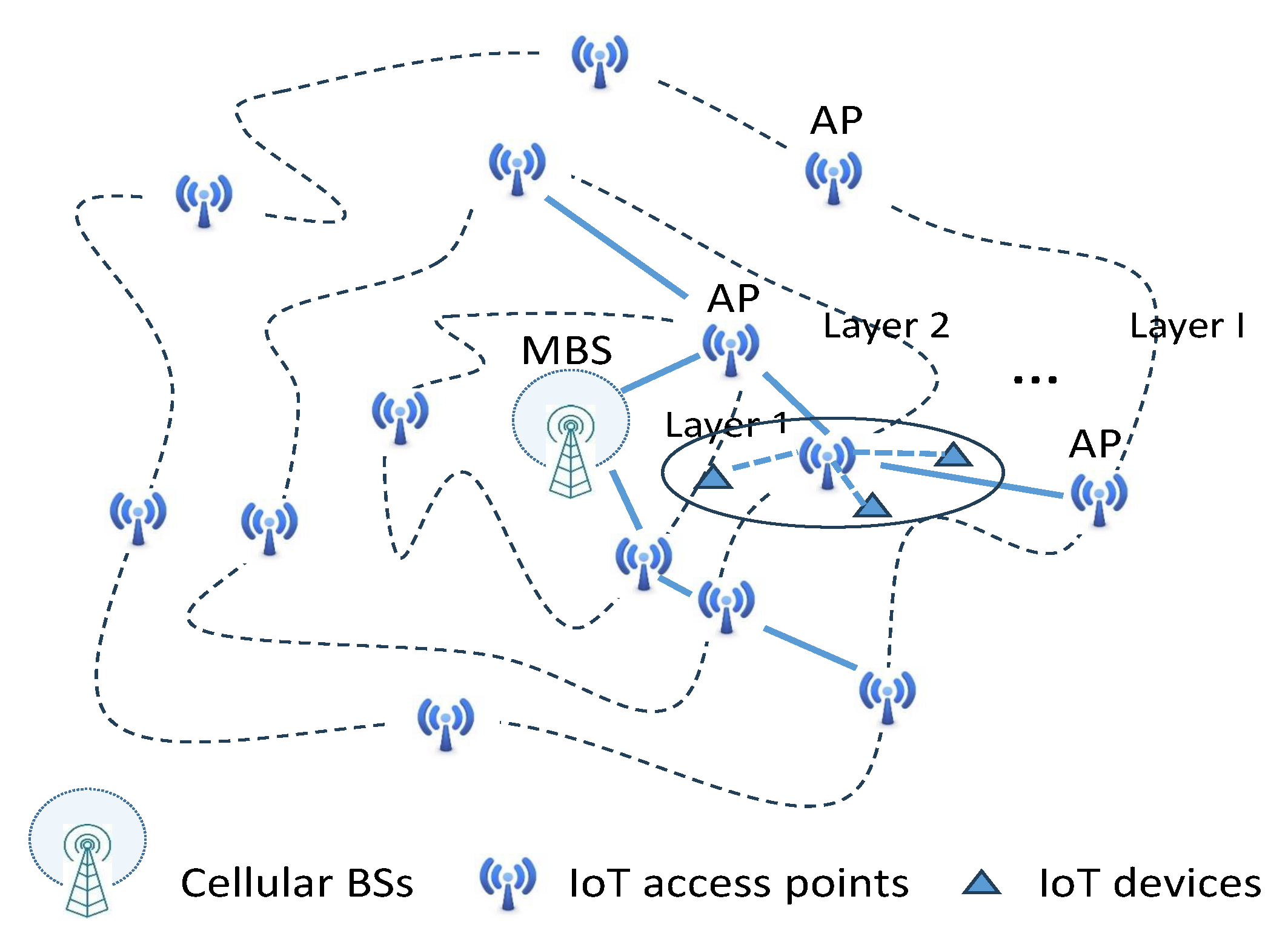
3. System Model

In this paper, we investigate a cellular-based IoT network with multi-tier APs, which is denoted by a graph $\mathbf{G}(\{\mathbf{M},\mathbf{A}\},\mathbf{D})$. In $\mathbf{G}$, $\mathbf{M}=\{m_1,\dots ,m_M\}$ is the set of M MBSs, $\mathbf{A}=\{a_1,\dots ,a_A\}$ is the set of A APs, and $\mathbf{D}=\{d_1,\dots ,d_D\}$ is the set of D IoT devices. The nodes in $\mathbf{M}$, $\mathbf{A}$ and $\mathbf{D}$ follow Poisson point process (PPP) distribution with intensities ${\delta }_m$, ${\delta }_a$, and ${\delta }_d$. The IoT devices transmit data packets to the corresponding MBS through several AP relays due to the limited transmission range in IoT networks. Then, as shown in Figure 1, each AP tier in the network consists of the APs with the same number of transmission counts from the MBS.

3.1. Channel Model

In cellular-based IoT networks, the communication environment is complex, and it is impossible to achieve ideal LOS communication channels for all the IoT devices, even with the utilization of multi-tier APs to extend network coverage and improve network connectivity. To achieve reliable analysis results for general communication scenarios, this paper models propagation channels by considering LOS and non-LOS components along with their occurrence probabilities separately in (1). The LOS connection probability is decided by the communication environment, height, and density of surrounding buildings, and the elevation angle between the IoT devices and APs along locations of them [18]. Depending on the LOS or non-LOS connection between the IoT device and AP, the received power $p_{j{j}^{\prime }}^r$ at node $j^{\prime }$ from node j is shown as

$$p_{j{j}^{\prime }}^r=\left\{\begin{array}{c}{p}_{j{j}^{\prime }}^t{g}_{j{j}^{\prime }}{d}_{j{j}^{\prime }}^{-\alpha },\mathrm{LOS} \mathrm{link},\hfill \\ \eta p_{j{j}^{\prime }}^t{g}_{j{j}^{\prime }}{d}_{j{j}^{\prime }}^{-\alpha },\mathrm{Non}\text{-}\mathrm{LOS} \mathrm{link},\hfill \end{array}\right.$$

(1)

where $\eta$ is an additional attenuation factor due to the non-LOS connection and $\forall j,j^{\prime }\in \mathbf{M}\cup \mathbf{A}\cup \mathbf{D},j\ne j^{\prime }$.

This paper utilizes the Rayleigh fading model in non-LOS paths for both desired signal and interference to achieve reliable analysis results in general communication scenarios, which leads to a random channel power gain following an exponential distribution with unit mean. Then the received power at node $j^{\prime }$ from node j, $p_{j{j}^{\prime }}^r$, is shown as [16]

$$p_{j{j}^{\prime }}^r=p_{j{j}^{\prime }}^t{g}_{j{j}^{\prime }}{d}_{j{j}^{\prime }}^{-\alpha },\forall j,j^{\prime }\in \mathbf{M}\cup \mathbf{A}\cup \mathbf{D},j\ne j^{\prime }$$

(2)

where power transmitted from node j to node $j^{\prime }$ is the $p_{j{j}^{\prime }}^t$. The $g_{j{j}^{\prime }}$ is a random variable that follows an exponential distribution with mean $\frac{1}{h}$ to account for the multi-path fading. Path loss exponent is $\alpha$. $d_{j{j}^{\prime }}=\sqrt{|x_j-x_j^{\prime }{|}^2+|y_j-y_j^{\prime }{|}^2+{|z_j-z_j^{\prime }|}^2}$ is the distance between node j and node $j^{\prime }$, where $(x_j,y_j,z_j)$ and $(x_{j^{\prime }},y_{j^{\prime }},z_{j^{\prime }})$ denote locations of node j and node $j^{\prime }$ in the Voronoi tessellation [19].

The transmission rate $C_{j{j}^{\prime }}$ from node j to node $j^{\prime }$ is

$$\begin{array}{c}\hfill C_{j{j}^{\prime }}=b_{j{j}^{\prime }}{log}_2(1+\frac{p_{j{j}^{\prime }}^r}{Ic+N_0}),\end{array}$$

(3)

where the channel bandwidth between j and $j^{\prime }$ is $b_{j{j}^{\prime }}$ with the co-channel interference and white Gaussian noise are $Ic$ and $N_0$.

3.2. Multi-Tier Cellular-Based IoT Network Model

In a cellular-based IoT network, the expected number of APs covered by one MBS can be given in the Poisson–Voronoi (PV) system, as shown in [19,20]

$$\begin{array}{c}\hfill E[N_a^m]={\delta }_{a}2\pi {\int }_0^{\infty }{l}_m{e}^{-{\delta }_m\pi l_m^2}d{l}_m=\frac{{\delta }_a}{{\delta }_m},\end{array}$$

(4)

where the radius of MBS cell coverage is $l_m$. By utilizing the same methodology, the expected number of IoT devices in one AP coverage $E[N_a^d]=\frac{{\delta }_d}{{\delta }_a}$.

With modifications in (4), the expected total length of connections between APs and MBS is as shown as

$$\begin{array}{c}\hfill E[L_a^m]={\delta }_{a}2\pi {\int }_0^{\infty }{l}_m^2{e}^{-{\delta }_m\pi l_m^2}d{l}_m=\frac{{\delta }_a}{2{{\delta }_m}^{\frac{3}{2}}},\end{array}$$

(5)

and expected total length of connections from device to AP is $E[L_d^a]=\frac{{\delta }_d}{2{{\delta }_a}^{\frac{3}{2}}}$.

The expected average length of connections between APs and MBS can be turned into the radius of MBS cell coverage, which can be given by utilizing the properties of Voronoi properties mentioned above:

$$\begin{array}{c}\hfill E[l_m]=\frac{E[L_a^m]}{E[N_a^m]}=\frac{\frac{{\delta }_a}{2{{\delta }_m}^{\frac{3}{2}}}}{\frac{{\delta }_a}{{\delta }_m}}=\frac{1}{2{{\delta }_m}^{\frac{1}{2}}}.\end{array}$$

(6)

Then, the mean number of tiers of APs covered by one MBS is

$$\begin{array}{c}\hfill I=\lceil \frac{E[l_m]}{r_{min}}\rceil ,\end{array}$$

(7)

where $r_{min}$ is the distance between neighboring tiers of APs, which is determined by the minimum transmission range needed to avoid co-channel interference.

By taking the same procedure as shown in (4), mean number of APs at the ith tier of AP network is represented as [20]

$$\begin{array}{cc}\hfill E[N_i^a]& =\frac{{\delta }_a}{{\delta }_m}(e^{-{\delta }_m\pi {(i{r}_{min})}^2}-e^{-{\delta }_m\pi {((i+1)r_{min})}^2}),\hfill \end{array}$$

(8)

where $i\in \{1,\dots ,(I-1)\}$.

3.3. Queueing Model in Multi-Tier Cellular-Based IoT Network

As shown in the multi-tier cellular-based IoT network model, each AP at the ith tier receives packets not only directly from the IoT device served by it but also from APs at the $(i+1)$th tier for relaying. To utilize the limited resources efficiently while considering the QoS requirement of the delay-sensitive IoT devices and the corresponding applications, we utilize different access protocols for different data traffic streams in the queueing model. The priority of each data packet is shown as

$$\begin{array}{c}\hfill {pri}_q=1-\frac{{AoI}_q}{{Delay}_{thr}^q},\end{array}$$

(9)

where $q\in \{1,\dots ,Q\}$ are the data packets in the waiting list to access the channel. The data packet that has the highest priority is named $q_1$, and the others with different sequence numbers from $\{2,\dots ,Q\}$, to indicate the priorities.

Data packet $q_1$ with the highest priority in the queueing model immediately occupies the channel as soon as the channel is sensed to be idle without the LBT procedure, while the other packets follow the CSMA/CA mechanism in the same batch. After the packet $q_1$ is successfully transmitted, the data packet with the highest priority among all the remaining data packets that not have been successfully transmitted yet follows the CSMA/CA mechanism in the next sensing process. In this paper, we name the data packet $q_1$ with the highest priority as a packet with priority and the other packets as packets without priority.

For the data received from the APs at the $(i+1)$th tier, the priority of each packet is decided by the location of the AP that the generating device is attached to, which is because the packet generated by the device attached to the APs far from the ith tier already experienced delay, which makes it more emergent to give priority to it to satisfy the QoS requirement by utilizing a shorter contention window size for these packets than that of the packets near the ith tier.

3.4. Mean Packet Delay of Packet with Priority

3.4.1. Without Packets in the Channel

The packet service time of packets with priority is determined by the status of the packets without priority. Under the average fraction of time that packets without priority do not occupy the channel, packets with priority in the queueing instantly occupy the channel, and the packet service time in this case is as shown as [17]

$$\begin{array}{c}\hfill S_{s,case1,1}=S_{s,o},\end{array}$$

(10)

where there is no packet with priority occupying the channel at the moment. $S_{s,o}$ is the channel occupancy time in service of packets with priority, and that for packets without priority is $S_{r,o}$. $S_{s,o}$ and $S_{r,o}$ follow the exponential distribution with $E[S_{s,o}]=\frac{1}{{\mu }_s}$ and $E[S_{r,o}]=\frac{1}{{\mu }_r}$, respectively. Packet arrival rates for packets with priority and packets without priority are ${\lambda }_s$ and ${\lambda }_r$, which follow Poisson distribution, respectively.

On the other hand, the packet service time of packets with priority with existing packets with priority occupying the channel is given by

$$\begin{array}{c}\hfill S_{s,case1,2}=R_{s,busy}+S_{s,o},\end{array}$$

(11)

where $R_{s,busy}$ is the residual busy period of packets with priority, whose Laplace–Stieltjes transform (LST) is as shown as [21]

$$\begin{array}{c}\hfill {\tilde{R}}_{s,busy}(s^{*})=\frac{{\mu }_s}{s^{*}+{\lambda }_s-{\lambda }_s{\tilde{B}}_s(s^{*})+{\mu }_s}{({\tilde{B}}_s(s^{*}))}^{{\lambda }_{s}E[S_s]}.\end{array}$$

(12)

The LSTs of $B_s$ based on the $S_{s,case1,1}$ are expressed as follows:

$$\begin{array}{c}\hfill {\tilde{B}}_s(s^{*})=\frac{{\mu }_s}{s^{*}+{\lambda }_s-{\lambda }_s{\tilde{B}}_s(s^{*})+{\mu }_s},\end{array}$$

(13)

where ${\tilde{B}}_s(s^{*})$ is a root of quadratic equation.

The mean packet service time of packets with priority in this case is

$$\begin{array}{cc}\hfill S_{s,case1}& =(1-{\lambda }_{s}E[S_{s,o}])S_{s,case1,1}+{\lambda }_{s}E[S_{s,o}]S_{s,case1,2}\hfill \\ \hfill & ={\lambda }_{s}E[S_{s,o}]R_{s,busy}+S_{s,o}.\hfill \end{array}$$

(14)

3.4.2. With Packets in the Channel

In addition, under the average fraction of time that packets without priority occupy the channel, packets with priority wait until the channel is released and occupy the channel as soon as the channel is sensed to be idle. The packet service time in this case is given by

$$\begin{array}{c}\hfill S_{s,case2}=R_{r,o}+S_{s,o},\end{array}$$

(15)

where $R_{r,o}$ is the residual service time of $S_{r,o}$. It is worth mentioning that this case is based on the fact that it is impossible to have packets with priority occupying the channel under the assumptions in this case.

Then, based on the fundamental theorem, the packet service time of packets with priority is shown as

$$\begin{array}{cc}\hfill S_s& =(1-{\lambda }_{r}E[S_{r,o}])S_{s,case1}+{\lambda }_{r}E[S_{r,o}]S_{s,case2}\hfill \\ \hfill & \stackrel{(\mathrm{a})}{=}\frac{{\lambda }_s}{{\mu }_s}{S}_{s,o}+S_{s,o}-\frac{{\lambda }_r}{{\mu }_r}\frac{{\lambda }_s}{{\mu }_s}{S}_{s,o}+\frac{{\lambda }_r}{{\mu }_r}{S}_{r,o}\hfill \\ \hfill & =\frac{{\lambda }_r}{{\mu }_r}{S}_{r,o}+S_{s,o},\hfill \end{array}$$

(16)

where $(a)$ is achieved by utilizing the memoryless property of exponential distribution.

The LST of $S_s$ can be given as

$$\begin{array}{cc}\hfill {\tilde{S}}_s(s^{*})& ={\tilde{S}}_{s,o}(s^{*}){\tilde{S}}_{r,o}(\frac{{\lambda }_r}{{\mu }_r}{s}^{*}){\tilde{R}}_{s,busy}(\frac{{\lambda }_s}{{\mu }_s}(1+\frac{{\lambda }_r}{{\mu }_r})s^{*})\hfill \\ \hfill & =\frac{{\mu }_s}{s^{*}+{\mu }_s}\frac{{\mu }_r}{\frac{{\lambda }_r}{{\mu }_r}{s}^{*}+{\mu }_r}{\tilde{R}}_{s,busy}(\frac{{\lambda }_s}{{\mu }_s}(1+\frac{{\lambda }_r}{{\mu }_r})s^{*})\hfill \\ \hfill & =(\frac{{\mu }_s}{s+{\mu }_s})(\frac{\frac{{\mu }_r^2}{{\lambda }_r}}{s+\frac{{\mu }_r^2}{{\lambda }_r}}).\hfill \end{array}$$

(17)

3.5. Mean Packet Delay of Packets without Priority

3.5.1. Without Packets with Priority in the Channel

By taking the analysis procedure as shown in the previous section for packets with priority, the packet service time of packets without priority at the ith tier of the multi-tier cellular-based IoT network can be achieved based on the status of packets with priority. In the case that packets with priority do not take the channel, the packet service time of packets without priority is [17]

$$\begin{array}{c}\hfill S_{r,case1,1}=S_{DIFS}+S_{back}+S_{r,o},\end{array}$$

(18)

where $S_{DIFS}$ is the time for successful completion of the distributed coordination function (DCF) inter-frame space (DIFS) without any packets with priority arriving. We also assume that there are no packets without priority occupying the channel in this case at the moment. However, if the channel is occupied during the duration of the DIFS, a new DIFS restarts after the channel is idle again, which can be given as a summation of stopped time for the time between the first DIFS starts and the last DIFS duration $T_{stop,DIFS}$ with a busy period of packets with priority $B_s$. Then the $S_{DIFS}$ analyzed above for packets without priority with CSMA/CA mechanism is [22], as shown in (19).

$$\begin{array}{cc}\hfill S_{DIFS}=& T_{DIFS}+\sum _{k=1}^{\infty }((T_{stop,DIFS,s}+B_s)P{r}_{k,arr,DIFS}^s+(T_{stop,DIFS,I}+B_I)P{r}_{k,arr,DIFS}^I\hfill \\ \hfill & +(T_{stop,DIFS,(I-1)}+B_{(I-1)})P{r}_{k,arr,DIFS}^{(I-1)}+(T_{stop,DIFS,(I-2)}+B_{(I-2)})P{r}_{k,arr,DIFS}^{(I-2)}\hfill \\ \hfill & +\dots +(T_{stop,DIFS,(i+3)}+B_{(i+3)})P{r}_{k,arr,DIFS}^{(i+3)}+(T_{stop,DIFS,(i+2)}+B_{(i+2)})P{r}_{k,arr,DIFS}^{(i+2)}).\hfill \end{array}$$

(19)

In (19), the $P{r}_{k,arr,DIFS}^{(i+2)}$ is

$$\begin{array}{c}\hfill P{r}_{k,arr,DIFS}^{(i+2)}=(1-P{r}_{k,arr,DIFS}^s)(1-P{r}_{k,DIFS,I})(1-P{r}_{k,DIFS,(I-1)})\dots (1-P{r}_{k,DIFS,(i+3)})P{r}_{k,DIFS,(i+2)},\end{array}$$

(20)

and $P{r}_{k,arr,DIFS}$ is the probability that there are arriving packets within the kth DIFS attempt duration.

The LST of $T_{stop,DIFS}$ and $B_s$ are as shown as follows:

$$\begin{array}{cc}\hfill {\tilde{T}}_{stop,DIFS}(s^{*})=& \frac{{\lambda }_s}{s^{*}+{\lambda }_s}\frac{1-e^{-(s^{*}+{\lambda }_s)T_{DIFS}}}{1-e^{-{\lambda }_s{T}_{DIFS}}}\frac{{\lambda }_I}{s^{*}+({\lambda }_s+{\lambda }_I)}\frac{1-e^{-(s^{*}+({\lambda }_s+{\lambda }_I))T_{DIFS}}}{1-e^{-{\lambda }_I{T}_{DIFS}}}\hfill \\ & \dots \frac{{\lambda }_{i+1}}{s^{*}+({\lambda }_s+{\lambda }_I+\dots +{\lambda }_{i+1})}\frac{1-e^{-(s^{*}+({\lambda }_s+{\lambda }_I+\dots +{\lambda }_{i+1}))T_{DIFS}}}{1-e^{-{\lambda }_{i+1}{T}_{DIFS}}},\hfill \end{array}$$

(21)

and

$$\begin{array}{c}\hfill {\tilde{B}}_s(s^{*})=(\frac{{\mu }_s}{s^{*}+{\lambda }_s-{\lambda }_s{\tilde{B}}_s(s^{*})+{\mu }_s})(\frac{\frac{{\mu }_r^2}{{\lambda }_r}}{s^{*}+{\lambda }_s-{\lambda }_s{\tilde{B}}_s(s^{*})+\frac{{\mu }_r^2}{{\lambda }_r}}),\end{array}$$

(22)

where the ${\tilde{B}}_s(s^{*})$ is a root of cubic equation.

Then, the LST of $S_{DIFS}$ is shown as

$$\begin{array}{cc}\hfill {\tilde{S}}_{DIFS}(s^{*})=& {\tilde{T}}_{DIFS}(s^{*}){\tilde{T}}_{stop,DIFS}((e^{{\lambda }_s{T}_{DIFS}}-1)(1+P{r}_{n-s,DIFS}+P{r}_{n-s,DIFS}P{r}_{n-{(k+1)}^{th},DIFS}+\dots +\hfill \\ \hfill & P{r}_{n-s,DIFS}P{r}_{n-{(k+1)}^{th},DIFS}\dots P{r}_{n-{(I-1)}^{th},DIFS})s^{*}){\tilde{B}}_s((e^{{\lambda }_s{T}_{DIFS}}-1)(1+P{r}_{n-s,DIFS}\hfill \\ \hfill & +P{r}_{n-s,DIFS}P{r}_{n-{(k+1)}^{th},DIFS}+\dots +P{r}_{n-s,DIFS}P{r}_{n-{(k+1)}^{th},DIFS}\dots P{r}_{n-{(I-1)}^{th},DIFS})s^{*}).\hfill \end{array}$$

(23)

$S_{back}$ is the time for the backoff procedure in the CSMA/CA mechanism. After detecting the channel is not occupied for the DIFS duration, the station initiates the transmission only if the channel remains idle for an additional random time duration $S_{back}$, which is determined by the contention window size and is given by

$$\begin{array}{c}\hfill S_{back}=T_{back}+N_{back,s}(B_s+S_{DIFS,s})+N_{back,i+1}(B_{i+1}+S_{DIFS,i+1})+\dots +N_{back,I}(B_I+S_{DIFS,I}),\end{array}$$

(24)

where $T_{back}$ is the backoff interval and $N_{back,s}$ is the number of arriving packets with priority during $T_{back}$. $N_{back,i+1}$ is the number of arriving packets without priority transmitted from devices served by APs at the $(i+1)$th tier.

Then, the LST of $S_{back}$ can be given by

$$\begin{array}{cc}\hfill {\tilde{S}}_{back}(s^{*})=& {\tilde{T}}_{back}(s^{*}){({\tilde{B}}_s(s^{*}){\tilde{S}}_{DIFS}(s^{*}))}^{N_{back,s}}({\tilde{B}}_{i+1}(s^{*})\hfill \\ \hfill & {\tilde{S}}_{DIFS,i+1}(s^{*}){)}^{N_{back,i+1}}\dots {({\tilde{B}}_I(s^{*}){\tilde{S}}_{DIFS,I}(s^{*}))}^{N_{back,I}}.\hfill \end{array}$$

(25)

On the other hand, the packet service time of packets without priority with existing packets without priority occupying the channel is given by

$$\begin{array}{c}\hfill S_{r,case1,2}=R_{r_o,busy}+S_{r,case1,1},\end{array}$$

(26)

where $R_{r_o,busy}$ is the residual busy period of packets without priority occupying the channel, whose LST is shown as

$$\begin{array}{c}\hfill {\tilde{R}}_{r_o,busy}(s^{*})=\frac{{\mu }_{r_o}}{s^{*}+{\lambda }_{r_o}-{\lambda }_{r_o}{\tilde{B}}_{r_o}(s^{*})+{\mu }_{r_o}}{({\tilde{B}}_{r_o}(s^{*}))}^{{\lambda }_{r_o}E[S_{r_o}]}.\end{array}$$

(27)

The LSTs of $B_{r_o}$ are expressed as follows:

$$\begin{array}{c}\hfill {\tilde{B}}_{r_o}(s^{*})=(\frac{{\mu }_{r_o}}{s^{*}+{\lambda }_{r_o}-{\lambda }_{r_o}{\tilde{B}}_{r_o}(s^{*})+{\mu }_{r_o}})(\frac{\frac{{\mu }_r^2}{{\lambda }_r}}{s^{*}+{\lambda }_{r_o}-{\lambda }_{r_o}{\tilde{B}}_{r_o}(s^{*})+\frac{{\mu }_r^2}{{\lambda }_r}}),\end{array}$$

(28)

where $r_o$ is the packets without priority occupying the channel. ${\tilde{B}}_{r_o}(s^{*})$ is a root of cubic equation.

Then, the mean packet service time of packets without priority in this case is shown as

$$\begin{array}{cc}\hfill S_{r,case1}& =(1-{\lambda }_{r}E[S_{r,o}])S_{r,case1,1}+{\lambda }_{r}E[S_{r,o}]S_{r,case1,2}\hfill \\ \hfill & ={\lambda }_{r}E[S_{r,o}]R_{r,busy}+S_{r,case1,1}.\hfill \end{array}$$

(29)

3.5.2. With Packets with Priority in the Channel

The packet service time of packets without priority in the case that packets with priority occupy the channel is presented as

$$\begin{array}{c}\hfill S_{r,case2}=R_{s,busy}+S_{r,case1,1}.\end{array}$$

(30)

It is also worth mentioning that this case is based on the fact that it is impossible to have packets without priority occupying the channel under the assumptions in this case.

Then based on the fundamental theorem, the packet service time of packets without priority is shown as

$$\begin{array}{cc}\hfill S_r=& (1-{\lambda }_{s}E[S_{s,o}])S_{r,case1}(T_{back},N_{back,s})+{\lambda }_{s}E[S_{s,o}]S_{r,case2}(T_{back},N_{back,s})\hfill \\ \hfill =& S_{DIFS}+S_{back}(T_{back},N_{back,s})+S_{r,o}+\frac{{\lambda }_s}{{\mu }_s}{R}_{s,busy}+\frac{{\lambda }_r}{{\mu }_r}(1-\frac{{\lambda }_s}{{\mu }_s})R_{r,busy}.\hfill \end{array}$$

(31)

The LST of $S_r$ is

$$\begin{array}{cc}\hfill {\tilde{S}}_r(s^{*})=& {\tilde{S}}_{DIFS}(s^{*}){\tilde{S}}_{back}(s^{*}|T_{back},N_{back,s}){\tilde{S}}_{r,o}(s^{*}){\tilde{R}}_{s,busy}(\frac{{\lambda }_s}{{\mu }_s}{s}^{*}){\tilde{R}}_{r,busy}(\frac{{\lambda }_r}{{\mu }_r}(1-\frac{{\lambda }_s}{{\mu }_s})s^{*}).\hfill \end{array}$$

(32)

4. Problem Formulation

4.1. Mean Packet Arrival Rate

In this paper, the successful transmission probability between the device and AP is $\beta$, then the mean packet arrival rate of packets with priority from the device to the serving AP ${\lambda }_s$ is

$$\begin{array}{c}\hfill {\lambda }^{uv}=E[N_u^v]C^{uv}\beta ,\end{array}$$

(33)

where $C^{uv}$ is the transmission rate from one device to the serving AP.

Then, the mean packet arrival rate in any AP at the ith tier of a multi-tier cellular-based IoT network is given by

$$\begin{array}{c}\hfill {\lambda }_i^v={\lambda }_s+{\lambda }_r={\lambda }_s+\frac{E[N_{(i+1)}^v]}{E[N_i^v]}{\mu }_{(i+1)}^v.\end{array}$$

(34)

If i equals I, then ${\lambda }_i^v={\lambda }^{uv}$. The ${\mu }_{(i+1)}^v$ is the mean service rate for packets in any AP at the $(i+1)$th tier of the network, which is also the packet transmission rate of packets without priority from any AP at the $(i+1)$th tier to APs at the ith tier, $C_{(i+1)}^{vv}$.

4.2. Mean Packet Transmission Delay

If we utilize the M/G/1 queue in each AP, the mean waiting time of packets in a random AP at the ith tier $E[W_i^v|N_i^v,\mathbf{b},\mathbf{p}]$ with given $N_i^v$, $\mathbf{b}$ and $\mathbf{p}$ is shown in the following [23]:

$$\begin{array}{c}\hfill E[W_i^v|N_i^v,\mathbf{b},\mathbf{p}]=E[L_i^v]E[S_i^v|N_i^v,\mathbf{b},\mathbf{p}]+{\rho }_i^{v}E[R_i^v|N_i^v,\mathbf{b},\mathbf{p}],\end{array}$$

(35)

where $E[L_i^v]$ is the number of packets in any AP at the ith tier and ${\rho }_i^v=\frac{{\lambda }_i^v}{{\mu }_i^v}$ is utility ratio. $E[S_i^v|N_i^v,\mathbf{b},\mathbf{p}]$ and $E[R_i^v|N_i^v,\mathbf{b},\mathbf{p}]$ are mean service time and residual service time, respectively. The $\mathbf{b}$ and $\mathbf{p}$ are spectrum and power allocation ratios for each tier in a multi-tier cellular-based IoT network. At each tier, spectrum and power are uniformly allocated to APs. The condition that ${\rho }_i^v\le 1$ must be satisfied to ensure the stability of the queue system. For convenience, the superscript v is removed for all parameters without any ambiguity.

With Little’s law and the relationship between service time and residual service time, which is

$$\begin{array}{c}\hfill E[R_i|N_i,\mathbf{b},\mathbf{p}]=E[S_i^2|N_i,\mathbf{b},\mathbf{p}]/2E[S_i|N_i,\mathbf{b},\mathbf{p}],\end{array}$$

(36)

the mean waiting time in (35) can be also represented as

$$\begin{array}{c}\hfill E[W_i|N_i,\mathbf{b},\mathbf{p}]=\frac{{\rho }_{i}E[S_i^2|N_i,\mathbf{b},\mathbf{p}]}{2(1-{\rho }_i)E[S_i|N_i,\mathbf{b},\mathbf{p}]}.\end{array}$$

(37)

Then, the mean packet transmission delay in a random AP at the ith tier, $E[D_i|N_i,\mathbf{b},\mathbf{p}]$, is given by

$$\begin{array}{c}\hfill E[D_i|N_i,\mathbf{b},\mathbf{p}]=E[S_i|N_i,\mathbf{b},\mathbf{p}]+\frac{{\rho }_{i}E[S_i^2|N_i,\mathbf{b},\mathbf{p}]}{2(1-{\rho }_i)E[S_i|N_i,\mathbf{b},\mathbf{p}]}.\end{array}$$

(38)

$E[S_i|N_i,\mathbf{b},\mathbf{p}]$ and $E[S_i^2|N_i,\mathbf{b},\mathbf{p}]$ are the first and second moments of conditional packet service time and can be obtained by applying the property of LST, which can be given as

$$\begin{array}{c}\hfill E[S_i|N_i,\mathbf{b},\mathbf{p}]=-{\tilde{S}}_i^{\prime }(0|N_i,\mathbf{b},\mathbf{p})\end{array}$$

(39)

and

$$\begin{array}{c}\hfill E[S_i^2|N_i,\mathbf{b},\mathbf{p}]={(-1)}^2{\tilde{S}}_i^{″}(0|N_i,\mathbf{b},\mathbf{p}).\end{array}$$

(40)

4.3. Channel Occupancy Time in Service

In this paper, the packet transmission time from the ith tier to the $(i-1)$th tier is defined as the packet service time $S_i$, which is $E[S_i]=1/C_i$ for per unit length packet. The achievable packet transmission rate in any AP at the ith tier is shown as $C_i=\frac{b_i}{E[N_i]}{log}_2(1+\frac{g(p_i/E[N_i])r_{min}^{-\alpha }}{I{c}_i+N_0})$, where $b_i$ and $p_i$ are the total spectrum and power resources allocated to APs at the ith tier. Then the CDF of $S_i$ can be represented as

$$\begin{array}{c}\hfill F_{S_i}(t|N_i,\mathbf{b},\mathbf{p})=Pr[S_i<t|N_i,\mathbf{b},\mathbf{p}]]=Pr[g>\frac{(2^{\frac{E[N_i]}{b_{i}t}}-1)(I{c}_i+N_0)}{(p_i/E[N_i])r_{min}^{-\alpha }}].\end{array}$$

(41)

With the fact that g ∼ $exp(h)$ [24], we can obtain

$$\begin{array}{cc}\hfill Pr[g>\frac{(2^{\frac{E[N_i]}{b_{i}t}}-1)(I{c}_i+N_0)}{(p_i/E[N_i])r_{min}^{-\alpha }}]& =E_{I{n}_i}[g>\frac{(2^{\frac{E[N_i]}{b_{i}t}}-1)(I{n}_i+N_0)}{(p_i/E[N_i])r_{min}^{-\alpha }}|I{n}_i]\hfill \\ \hfill & \stackrel{(\mathrm{b})}{=}{e}^{-h\frac{(2^{\frac{E[N_i]}{b_{i}t}}-1)N_0}{(p_i/E[N_i])r_{min}^{-\alpha }}}{L}_{I{c}_i}(h\frac{(2^{\frac{E[N_i]}{b_{i}t}}-1)}{(p_i/E[N_i])r_{min}^{-\alpha }}),\hfill \end{array}$$

(42)

where the proof for (b) is given in Appendix A.

Then, the PDF of service time $S_i$ at the ith tier can be achieved:

$$\begin{array}{cc}\hfill f_{S_i}(t|N_i,\mathbf{b},\mathbf{p})& =\frac{d}{d_t}{F}_{S_i}(t|N_i,\mathbf{b},\mathbf{p})\hfill \\ \hfill & =\frac{d}{d_t}Pr[g>\frac{(2^{\frac{E[N_i]}{b_{i}t}}-1)(I{n}_i+N_0)}{(p_i/E[N_i])r_{min}^{-\alpha }}]\hfill \\ \hfill & ={(e^{-h\frac{(2^{\frac{E[N_i]}{b_{i}t}}-1)N_0}{(p_i/E[N_i])r_{min}^{-\alpha }}})}^{\prime }{L}_{I{c}_i}(h\frac{(2^{\frac{E[N_i]}{b_{i}t}}-1)}{(p_i/E[N_i])r_{min}^{-\alpha }})+e^{-h\frac{(2^{\frac{E[N_i]}{b_{i}t}}-1)N_0}{(p_i/E[N_i])r_{min}^{-\alpha }}}{L}_{I{c}_i}^{\prime }(h\frac{(2^{\frac{E[N_i]}{b_{i}t}}-1)}{(p_i/E[N_i])r_{min}^{-\alpha }})\hfill \end{array}$$

(43)

where ${(e^{-h\frac{(2^{\frac{E[N_i]}{b_{i}t}}-1)N_0}{(p_i/E[N_i])r_{min}^{-\alpha }}})}^{\prime }$ and $L_{I{c}_i}^{\prime }(h\frac{(2^{\frac{E[N_i]}{b_{i}t}}-1)}{(p_i/E[N_i])r_{min}^{-\alpha }})$ can be achieved by derivation operations.

$$\begin{array}{c}\hfill {(e^{-h\frac{(2^{\frac{E[N_i]}{b_{i}t}}-1)N_0}{(p_i/E[N_i])r_{min}^{-\alpha }}})}^{\prime }=e^{-h\frac{(2^{\frac{E[N_i]}{b_{i}t}}-1)N_0}{(p_i/E[N_i])r_{min}^{-\alpha }}}\frac{-h{N}_0}{(p_i/E[N_i])r_{min}^{-\alpha }}{2}^{\frac{E[N_i]}{b_{i}t}}(ln2)\frac{E[N_i]}{b_i}(-t^{-2})\end{array}$$

(44)

and $L_{I{c}_i}^{\prime }(h\frac{(2^{\frac{E[N_i]}{b_{i}t}}-1)}{(p_i/E[N_i])r_{min}^{-\alpha }})$ is shown as (45).

$$\begin{array}{cc}\hfill & L_{I{c}_i}^{\prime }(h\frac{(2^{\frac{E[N_i]}{b_{i}t}}-1)}{(p_i/E[N_i])r_{min}^{-\alpha }})=exp(-2\pi {\delta }_v{\int }_{r_{min}}^{\infty }\frac{\frac{(2^{\frac{E[N_i]}{b_{i}t}}-1)}{(p_i/E[N_i])}}{\frac{(2^{\frac{E[N_i]}{b_{i}t}}-1)}{(p_i/E[N_i])}+{(\frac{\tau }{r_{min}})}^{\alpha }}\tau d\tau )(-2\pi {\delta }_v)\hfill \\ & {\int }_{r_{min}}^{\infty }\frac{\frac{(2^{\frac{E[N_i]}{b_{i}t}}-1)}{(p_i/E[N_i])}(\frac{E[N_i]}{p_i})2^{\frac{E[N_i]}{b_{i}t}}(ln2)\frac{E[N_i]}{b_i}(t^{-2})-(\frac{E[N_i]}{p_i})2^{\frac{E[N_i]}{b_{i}t}}(ln2)\frac{E[N_i]}{b_i}(t^{-2})(\frac{(2^{\frac{E[N_i]}{b_{i}t}}-1)}{(p_i/E[N_i])}+{(\frac{\tau }{r_{min}})}^{\alpha })}{{(\frac{(2^{\frac{E[N_i]}{b_{i}t}}-1)}{(p_i/E[N_i])}+{(\frac{\tau }{r_{min}})}^{\alpha })}^2}\tau d\tau .\hfill \end{array}$$

(45)

With a conditional PDF of the service time, we can obtain the mean packet transmission delay in a random AP at the ith tier.

4.4. Total Packet Delay Minimization Problem

In multi-tier cellular-based IoT networks, it is essential to investigate mean total packet delay for packets due to the delay penalty to packets caused by the multi-hopping transmission, which is the summation of served delay and relayed delay experienced at each tier, and can be shown as follows:

$$\begin{array}{c}\hfill D_t=D_s+D_r=D_s+D_{r,(i-1)}+D_{r,(i-2)}+\dots +D_{r,1}.\end{array}$$

(46)

We present a cellular-based IoT network with APs in two tiers to demonstrate the effectiveness of the analysis results and then formulate a mean total packet delay minimization problem for packets transmitted from devices served by APs at the second tier of the IoT network. Then, the optimization problem with objective function and the corresponding constraints is shown as

$$\begin{array}{cccc}\hfill & \underset{\varphi ,\xi }{\min }\hfill & \hfill & E[D_t](\varphi ,\xi )\hfill \\ \hfill & \mathrm{s}.\mathrm{t}.\hfill & \hfill & \sum _{i=1}^2{b}_i=B,\sum _{i=1}^2{p}_i=P,\hfill \\ \hfill & \hfill & & {\rho }_{r,1}\le 1,{\rho }_{s,i}\le 1i\in \{1,2\},\hfill \\ \hfill & \hfill & & 0\le \varphi ,\xi \le 1,\hfill \end{array}$$

(47)

where $E[D_t]=E[D_{s,2}]+E[D_{r,1}]$. The total packet delay, $E[D_t]$, includes delay experienced as served packet at the second tier $E[D_{s,2}]$ and relayed packet at the first tier $E[D_{r,1}]$. The ratios of spectrum and power allocated to APs at the first tier are $\varphi$ and $\xi$, as $\varphi =\frac{b_1}{B}$ and $\xi =\frac{p_1}{P}$, respectively. The P and B are the total power and spectrum for the two tiers of APs, respectively.

The proposed algorithm for total packet transmission delay minimization via resources optimal allocation in the cellular-based IoT networks with multi-tier APs is exhibited in Algorithm 1 [25].

Algorithm 1: Proposed algorithm for total packet transmission delay minimization.

5. Numerical Results

In this paper, we present a cellular-based IoT network with two-tier APs in one MBS cell coverage with dimensions 1 km × 1 km × 1 km. The distance between two tiers of APs is 50 m. In the simulation, ${\delta }_m$, ${\delta }_a$ and ${\delta }_d$ are 1, 1000, and 10,000 per km${}^2$, respectively. The total spectrum and power for APs in the network are 1000 MHz and 100 W, respectively. The step size $\theta$ to update $\varphi$ and $\xi$ is $0.05$. The system parameter $T_{DIFS}$ is $36\times {10}^{-6}$ s, and the maximum $T_{back}$ is $72\times {10}^{-6}$ s by taking slot time as $9\times {10}^{-6}s$ with the contention window size as 8.

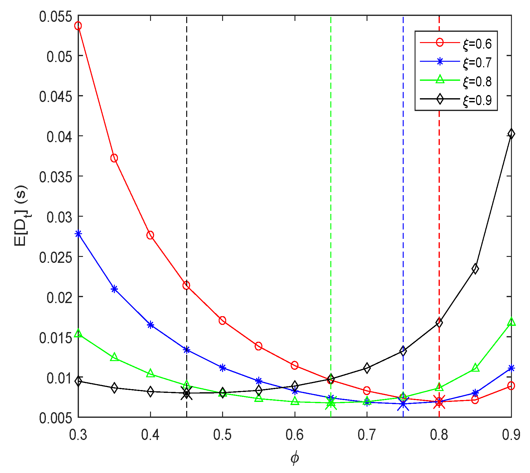
Figure 2 presents variation trends of the total packet transmission delay $E[D_t]$ as spectrum allocation ratio $\varphi$ for different fixed power allocation ratios $\xi$. Meanwhile, the minimum $E[D_t]$ for each $\xi$ reveals the optimal value of $\varphi$, which is ${\varphi }^{*}$ as shown with the vertical dotted lines. Based on the facts shown in the figure, we can observe that the value of ${\varphi }^{*}$ is decreasing as the $\xi$ keeps increasing, which is due to the fact that more transmission power can compensate the shortage of spectrum resource to achieve the same minimum total packet delay.

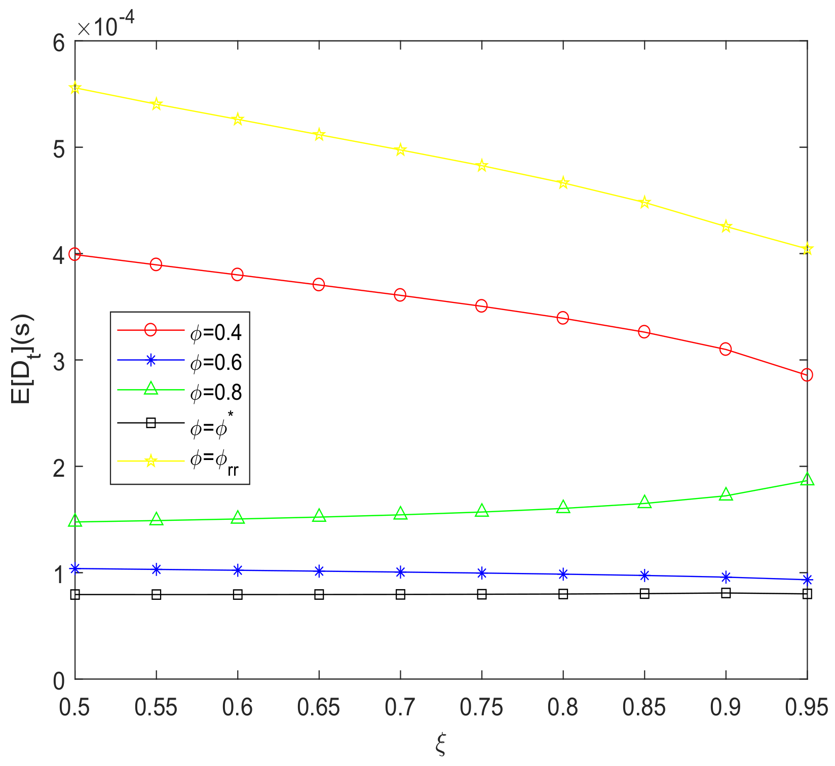
Figure 3 shows the variation trend of the total packet transmission delay $E[D_t]$ as power allocation ratio $\xi$ for various fixed values of spectrum allocation ratio $\varphi$. Also, the minimum $E[D_t]$ for each $\varphi$ reveals the optimal value of $\xi$, which is ${\xi }^{*}$ as shown with the vertical dotted lines. The value of ${\xi }^{*}$ is decreasing as the $\varphi$ keeps increasing, which reflects the same conclusion as shown in Figure 2 and cross-proves the correctness of the proposed scheme and algorithm. On the other hand, it presents a performance comparison of the proposed mechanism and the spectrum resource allocation with the Monte Carlo simulation. As shown in the figure, the proposed mechanism obtains better minimum mean total packet delay with ${\varphi }^{*}$ than the $\varphi$ is any other values obtained by using the Monte Carlo simulation. Meanwhile, the performance comparison of the proposed scheme with the spectrum allocation based on the round-robin scheduling mechanism with $\varphi ={\varphi }_{rr}$ by the total packet transmission delay is given in Figure 4. In the round-robin scheduling mechanism, each tier in the multi-tier cellular-based IoT network alternatively utilizes all the network resources, which results in a single-hop transmission network and accumulates all the network traffic. It also shows superior performance than the round-robin scheduling in the figure.

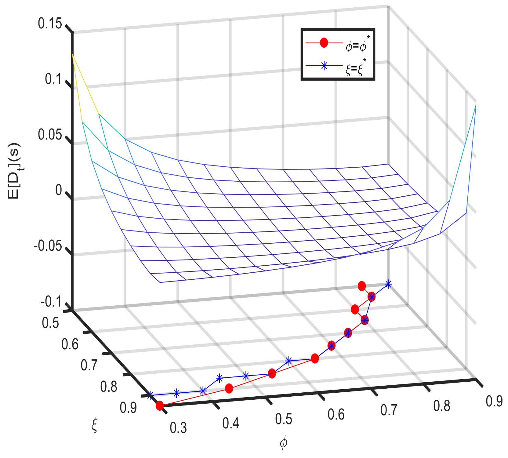
Based on the results shown in Figure 2 and Figure 3, Figure 5 describes the value of optimal $\xi$ and optimal $\varphi$, which collaboratively reveal the minimum $E[D_t]$ as shown in the third dimension in the figure. In the figure, the value of ${\xi }^{*}$ is decreasing with $\varphi$ increasing, and the value of ${\varphi }^{*}$ is decreasing when $\xi$ is increasing, as shown in Figure 2 and Figure 3. With the condition mentioned above that ${\rho }_i\le 1$ must be satisfied, $\xi$ cannot be less than $0.5$ in Figure 3 and Figure 5.

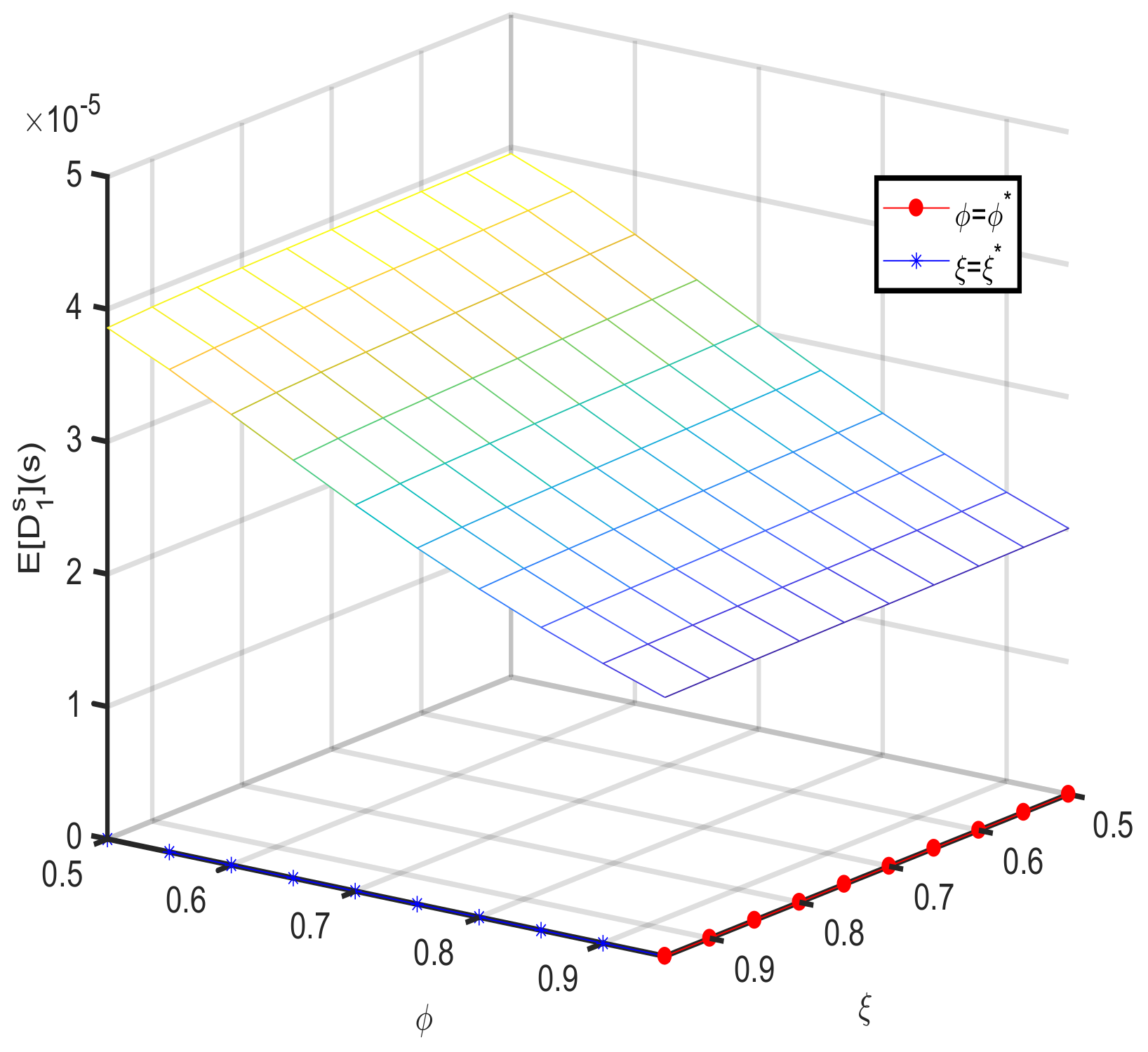
With Figure 5 as a basis, Figure 6 describes the mean delay $E[D_{s,1}]$ at the first tier of the network experienced by the packets transmitted from devices served by APs at the first tier of the multi-tier cellular-based IoT network. The optimal values of $\varphi$, ${\varphi }^{*}$, and the optimal value of $\xi$, ${\xi }^{*}$, are constant at the maximum values to achieve the minimum $E[D_{s,1}]$, as shown in Figure 6, on account of more spectrum and power resources leading to the smaller delay to packets from devices attached to the APs in the first tier with constant packets arrival rate and higher priority than the other packets.

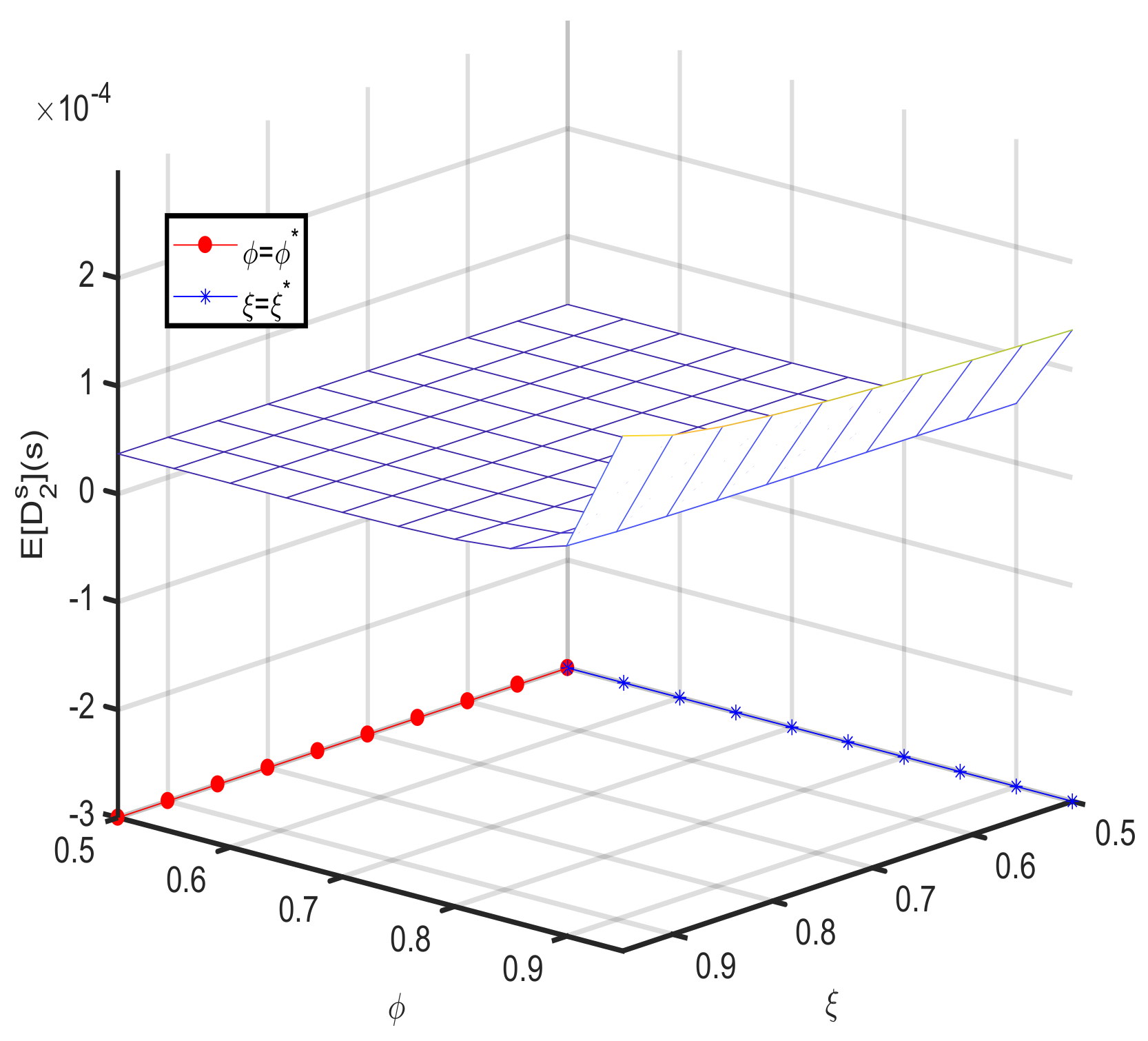
On the other hand, Figure 7 exhibits the mean delay $E[D_{s,2}]$ at the second tier of the network experienced by the packets transmitted from devices served by APs at the second tier of multi-tier cellular-based IoT networks. The optimal value of $\varphi$, ${\varphi }^{*}$, and the optimal value of $\xi$, ${\xi }^{*}$, is constant at the minimum values to obtain the minimum $E[D_{s,2}]$, as shown in Figure 7, for more spectrum and power resources.

Figure 8 shows the mean delay $E[D_{r,1}]$ at the first tier of the network experienced by the packets transmitted from devices served by APs at the second tier of the multi-tier cellular-based IoT networks for relaying. The optimal value of $\varphi$, ${\varphi }^{*}$, is constant at the maximum value, which is due to the relaying delay being the dominant factor in mean total packet delay and needs enough resources to guarantee the QoS performance due to the large AoI. The optimal value of $\xi$, ${\xi }^{*}$ decreases from the maximum value to the minimum value as $\varphi$ increases because the maximum power resource is needed to obtain the minimum mean relaying delay when the spectrum resource cannot be guaranteed, as the spectrum increases until it reaches the value where the minimum mean total packet delay can be guaranteed with any ratio of power resource allocation, which changes to minimum value sharply, and the remaining part is allocated to the second tier of the IoT network. It also shows that the mean total packet delay is more sensitive to $\xi$ compared to $\varphi$, because the mean delay for relaying is more sensitive to $\xi$, as shown.

6. Conclusions

In this paper, we proposed a multi-tier cellular-based IoT network with a traffic prioritization scheduling scheme based on the AoI metric to satisfy strict data packet latency requirements in 5G IoT networks. Our mathematical framework based on the queueing theory models the time-domain behaviors of data packets with different channel access protocols to overcome delay penalties and ensure fairness for packets with large AoI metrics. Then, we minimized the mean total packet delay by optimally distributing spectrum and power resources among multiple tiers in IoT networks. Numerical results demonstrated the effectiveness of the proposed mechanism and algorithm in a two-tier cellular-based IoT network, which achieved the minimum total packet transmission delay to meet strict latency requirements. Moreover, the optimal allocation of spectrum and power resources minimized delays of data packets experienced at each tier in the multi-tier IoT networks, which realized monitoring and guaranteeing the packet latency as a requirement in real-time. Future studies will consider a more general and practical case in which forwarded packets have different priorities based on the location of the transmitting device. Our work contributes to the development of IoT networks by addressing packet delay penalties during multi-hopping transmission and improving fairness for different kinds of data packets.

References

1. Sun, H.; Shen, H.; Yang, H.H.; Wang, X.; Liu, J.; Li, S.; Quek, T.Q.S. Impacts of User Association and Power Control on AoI in Multi-Tier Cellular-Based IoT Networks. IEEE Wirel. Commun. Lett. 2022, 11, 1196–1200. [Google Scholar] [CrossRef]
2. Jiang, N.; Deng, Y.; Nallanathan, A.; Kang, X.; Quek, T.Q.S. Analyzing Random Access Collisions in Massive IoT Networks. IEEE Trans. Wirel. Commun. 2018, 17, 6853–6870. [Google Scholar] [CrossRef]
3. Mankar, P.D.; Chen, Z.; Abd-Elmagid, M.A.; Pappas, N.; Dhillon, H.S. Throughput and Age of Information in a Cellular-Based IoT Network. IEEE Trans. Wirel. Commun. 2021, 20, 8248–8263. [Google Scholar] [CrossRef]
4. Park, J.; Kim, S.; Youn, J.; Ahn, S.; Cho, S. Low-Complexity Data Collection Scheme for UAV Sink Nodes in Cellular IoT Networks. IEEE Trans. Veh. Technol. 2021, 70, 4865–4879. [Google Scholar] [CrossRef]
5. Park, E.; Kim, T.; Han, Y. An Efficient Time-Shifted Random Access Scheme for Cellular-Based IoT Networks. IEEE Commun. Lett. 2019, 23, 522–525. [Google Scholar] [CrossRef]
6. Jiang, N.; Deng, Y.; Kang, X.; Nallanathan, A. Random Access Analysis for Massive IoT Networks Under a New Spatio-Temporal Model: A Stochastic Geometry Approach. IEEE Trans. Commun. 2018, 66, 5788–5803. [Google Scholar] [CrossRef]
7. Ebrahimi, D.; Sharafeddine, S.; Ho, P.-H.; Assi, C. UAV-Aided Projection-Based Compressive Data Gathering in Wireless Sensor Networks. IEEE Internet Things J. 2019, 6, 1893–1905. [Google Scholar] [CrossRef]
8. Abd-Elmagid, M.A.; Pappas, N.; Dhillon, H.S. On the Role of Age of Information in the Internet of Things. IEEE Commun. Mag. 2019, 57, 72–77. [Google Scholar] [CrossRef]
9. Cheikh, I.; Sabir, E.; Aouami, R.; Roy, S.; Sadik, M. Data Freshness and End-to-End Delay in Cross-Layer Two-Tier Linear IoT Networks. Sensors 2022, 22, 9455. [Google Scholar] [CrossRef]
10. Fu, S.; Jiang, D. Multi-Dimensional Resource Allocation for Throughput Maziximization in CRIoT with SWIPT. Energies 2023, 16, 4767. [Google Scholar] [CrossRef]
11. Zhao, J.; Mei, Y.; Gao, X.; Yang, J.; Shang, J. Multi-Objective Optimization for EE-SE Tradeoff in Space-Air-Ground Internet of Things Networks. Electronics 2023, 12, 2585. [Google Scholar] [CrossRef]
12. Ma, B.; Xu, D.; Ren, X.; Wang, Y.; Liu, J. Resource Allocation of UAV-Assisted IoT Node Secure Communication System. Signals 2023, 4, 591–603. [Google Scholar] [CrossRef]
13. Ramamoorthy, P.; Sanober, S.; Di Nunzio, L.; Cardarilli, G.C. Sustainable Power Consumption for Variance-Based Integration Model in Cellular 6G-IoT System. Sustainability 2023, 15, 12696. [Google Scholar] [CrossRef]
14. Kim, T.; Chae, S.; Lim, J.-T.; Bang, I. Resource-Efficient Parallelized Random Access for Reliable Connection Establishment in Cellular IoT Networks. Sensors 2023, 23, 3819. [Google Scholar] [CrossRef] [PubMed]
15. Tung, T.V.; An, T.T.; Lee, B.M. Joint Resource and Trajectory Optimization for Energy Efficiency Maximization in UAV-Based Networks. Mathematics 2022, 10, 3840. [Google Scholar] [CrossRef]
16. Li, J.; Han, Y. Optimal resource allocation for packet delay minimization in Multi-layer UAV networks. IEEE Commun. Lett. 2017, 21, 580–583. [Google Scholar] [CrossRef]
17. Li, J.; Han, Y. A traffic service scheme for delay minimization in Multi-Layer UAV networks. IEEE Trans. Veh. Technol. 2018, 67, 5500–5504. [Google Scholar] [CrossRef]
18. Mozaffari, M.; Saad, W.; Bennis, M.; Debbah, M. Unmanned aerial vehicle with underlaid device-to-device communications: Performance and tradeoffs. IEEE Trans. Wirel. Commun. 2016, 15, 3949–3963. [Google Scholar] [CrossRef]
19. Foss, S.G.; Zuyev, S.A. On a Voronoi Aggregative Process Related to a Bivariate Poisson Process. Adv. Appl. Probab. 1996, 28, 965–981. [Google Scholar] [CrossRef]
20. Jin, Z.; Kim, D.; Cho, J.; Lee, B. An Analysis on Optimal Cluster Ratio in Cluster-Based Wireless Sensor Networks. IEEE Sens. J. 2015, 15, 6413–6423. [Google Scholar] [CrossRef]
21. Wang, X.; Quek, T.Q.S.; Sheng, M.; Li, J. On the coexistence of Wi-Fi and LTE-U in unlicensed spectrum. In Proceedings of the 2017 IEEE International Conference on Communications (ICC), Paris, France, 21–25 May 2017. [Google Scholar]
22. Song, Y.; Sung, K.W.; Han, Y. Impact of packet arrivals on Wi-Fi and cellular system sharing unlicensed spectrum. IEEE Trans. Veh. Technol. 2016, 65, 10204–10208. [Google Scholar] [CrossRef]
23. Adan, I.; Resing, J. Queueing Theory; Department of Mathematics and Computer Science, Eindhoven University of Technology: Eindhoven, The Netherlands, 2001. [Google Scholar]
24. Renzo, M.D.; Lam, T.T.; Zappone, A.; Debbah, M. A Tractable Closed-Form Expression of the Coverage Probability in Poisson Cellular Networks. IEEE Wirel. Commun. Lett. 2018, 8, 249–252. [Google Scholar] [CrossRef]
25. Boyd, S.; Vandenberghe, L. Convex Optimization; Cambridge University Press: Cambridge, UK, 2004. [Google Scholar]
Figure 1. Multi-tier cellular-based IoT network model.
Mathematics 11 04538 g001
Figure 2. Total packet transmission delay E [ D t ] as a function of ϕ .
Mathematics 11 04538 g002
Figure 3. Total packet transmission delay E [ D t ] as a function of ξ .
Mathematics 11 04538 g003
Figure 4. Performance comparison for the proposed scheme.
Mathematics 11 04538 g004
Figure 5. The optimal ϕ and ξ for the minimum E [ D t ] .
Mathematics 11 04538 g005
Figure 6. The optimal ϕ and ξ for the minimum E [ D s , 1 ] .
Mathematics 11 04538 g006
Figure 7. The optimal ϕ and ξ for the minimum E [ D s , 2 ] .
Mathematics 11 04538 g007
Figure 8. The optimal ϕ and ξ for the minimum E [ D r , 1 ] .
Mathematics 11 04538 g008
Disclaimer/Publisher’s Note: The statements, opinions and data contained in all publications are solely those of the individual author(s) and contributor(s) and not of MDPI and/or the editor(s). MDPI and/or the editor(s) disclaim responsibility for any injury to people or property resulting from any ideas, methods, instructions or products referred to in the content.