Solving the Flying Sidekick Traveling Salesman Problem by a Simulated Annealing Heuristic

Abstract

This study investigates the flying sidekick traveling salesman problem (FSTSP), in which a truck and an unmanned aerial vehicle work together to make deliveries. This study develops a revised mixed-integer linear programming (MILP) model for the FSTSP. The revised MILP model performs better than the existing model. Due to the FSTSP’s high complexity, we propose an effective heuristic based on simulated annealing (SA) to solve the problem. The novelty of the proposed SA heuristic lies in the new solution representation, which not only determines the visiting sequence of customers but also the service type of customers and rendezvous positions. Another feature of the proposed SA is a new operator specifically designed for the FSTSP. To evaluate the performance of the proposed SA heuristic, we conduct a comprehensive computational study where we fine-tune the parameters of the SA heuristic and compare the performance of the SA heuristic with several state-of-the-art algorithms including hybrid genetic algorithm (HGA) and iterated local search (ILS) in solving existing FSTSP benchmark instances. The results indicate that the proposed SA heuristic outperforms ILS and is statistically competitive with HGA. It obtains best-known solutions for all small FSTSP instances and 29 best-known solutions for the 60 large FSTSP instances, including 20 new best-known solutions.

1. Introduction

As the e-commerce market expands, challenges that are encountered by logistics firms become more complex, particularly in the last-mile delivery. Companies need to meet customer expectations on shorter delivery times while demands grow higher [1]. According to [2], for many companies the transportation cost occurring in the last-mile parcel delivery often exceeds 50% of the total transportation cost.

To run a more cost-effective and efficient business to deliver goods to customers, logistics companies are looking for more advanced technology to enhance their last-mile delivery performance. Unmanned aerial vehicles (UAVs)—which are known as drone technology—have recently received attention from both companies and researchers to be utilized in a wide range of applications, such as forestry research [3], fisheries assessment and management [4], agriculture [5], disaster management [6,7], inspection and monitoring [8,9,10], and healthcare [11,12], to name a few. This emerging technology opens an opportunity for the last-mile delivery. Several advantages are offered, including that no costly human pilot is needed, and no congestion will occur for the travel of the drone [13].

The application of drone technology was initiated by several companies, pioneered by Amazon in 2013, where Amazon CEO Jeff Bezos first announced “Amazon Prime Air,” which utilized drones for delivery purposes [14]. A test was later conducted by Australia Post for delivering small packages [15]. DHL has also developed DHL Parcel to distribute emergency supplies and medications to one of Germany’s North Sea Islands [16]. Google’s parent company—Alphabet—has developed Project Wing to create a working drone delivery system [17].

Although drone technology provides new competitive advantages, several innate limitations, such as flight duration and flight restriction, are unavoidable. Therefore, a hybrid system integrating drone technology to regular truck delivery was developed to further extend the benefit of utilizing drones. This type of system was initially tested by AMP Electric Vehicles and the Department of Aerospace Engineering, University of Cincinnati [13]. Later, UPS successfully experimented the integration of the drone technology with UPS trucks [18].

The hybrid system between drone technology and regular truck delivery has started to gain attention from researchers and recently has given rise to several optimization problems proposed in the academic literature [19,20,21,22,23,24,25]. Murray and Chu [26] pioneered this stream of research. They proposed two new variants of the classical traveling salesman problem (TSP), incorporating drones with a delivery truck. One of the variants is the flying sidekick traveling salesman problem (FSTSP). When there are long distances between the depot and customers, the FSTSP is applicable to extend the coverage of the drones by collaborating with delivery trucks. In the FSTSP, each customer must be served precisely once by either a delivery truck or a drone working with the truck. Several customers are infeasible to be visited by a drone, and consequently they could only be visited by the truck. Minimizing the customer service time and disposition time of vehicles is the purpose of the FSTSP.

This study is motivated by the challenges and the practicality presented by the FSTSP. The problem is difficult to solve as it extends the TSP, an NP-hard problem. However, since the truck–drone delivery system is gaining popularity in practice, the FSTSP may become an essential optimization problem that needs to be effectively solved routinely. Therefore, an improved mixed-integer linear programming (MILP) model and an effective simulated annealing (SA) heuristic is developed in this study to solve the problem. Based on the computational results, our SA is competitive with the state-of-the-art algorithms for the FSTSP. Thus, the contribution of this study is two-fold:

• An improved MILP model for the FSTSP is formulated. The model is more compact and effective than the existing model of Murray and Chu [26].
• A simulated annealing algorithm is developed for the FSTSP. The proposed SA features a new solution representation and a new operator specifically designed for the FSTSP. It outperforms the iterative local search for the FSTSP and is competitive with the hybrid genetic algorithm for the FSTSP.

The remainder of the paper is organized as follows. Section 2 reviews the relevant literature. Section 3 describes the FSTSP and presents a new mixed-integer programming model for the problem. Section 4 discusses the proposed SA heuristic for solving the FSTSP. Section 5 presents the experimental results. Section 6 provides conclusions and points out potential directions for future studies.

2. Literature Review

Murray and Chu [26] pioneered the research on the integrated truck and drone delivery system by extending the TSP to become the FSTSP. A mixed-integer linear programming model was formulated for the problem. They also analyzed the influence of a drone’s speed and endurance toward the potential savings of these two models compared to the classical TSP in terms of makespan. Based on the conducted experiments, they showed that the speed has a significant impact, while the endurance seemingly shows no effect on the potential savings. The faster a drone is, the higher the potential saving that could be made.

The research on the integrated truck and drone delivery system started to gain momentum after the work of Murray and Chu [26]. Agatz, Bouman, and Schmidt [19] further improved the mathematical models of Murray and Chu [26] and successfully solved large instances to optimality. They also proposed a route-first, cluster-second heuristic of several versions to solve large instances since they could not solve their mathematical models to optimality. More recently, Dell’Amico et al. [27] proposed improved mathematical programming models for the FSTSP and Roberti and Ruthmair [28] provided a more compact mathematical model for several variants of TSP-D.

Several solution approaches have been proposed for solving the FSTSP. Exact algorithms such as the branch-and-bound algorithm [24] and branch-and-cut algorithm [27,29] were developed for the problem. Many heuristic algorithms were also proposed in recent years. De Freitas and Penna [30] developed a randomized variable neighborhood descent heuristic for solving the FSTSP. They first solved a TSP to build an initial solution and then improved the solution by the proposed RVND heuristic. Yurek and Ozmutlu [31] proposed a decomposition-based iterative optimization algorithm to solve the FSTSP in two stages. The first stage determines the truck route and the assignment of customers to the drone. The second stage solves a MILP to improve the solution obtained in the first stage. De Freitas and Penna [32] developed a variable neighborhood search (VNS) heuristic for the FSTSP. An initial solution is obtained by optimally solving a TSP. The proposed VNS is then applied to improve the initial solution. Ha et al. [33] proposed two algorithms for solving TSP-D. The first algorithm, TSP-LS, applies a local search procedure on an optimal TSP solution to obtain a feasible TSP-D solution. The second algorithm is a greedy randomized adaptive search procedure (GRASP). The experimental results suggest that GRASP outperforms TSP-LS. Ha et al. [34] developed a hybrid genetic algorithm (HGA) for TSP-D. The algorithm incorporates many features such as dynamic population management, adaptive diversity control, tailored crossover, and local search operators. The algorithm is competitive to two existing algorithms and finds many new best-known solutions. In Ha et al. [35], an iterated local search (ILS) was proposed to solve the TSP with a Multi-Visit Drone (TSP-MVD), in which a truck works in collaboration with a drone that can serve up to q ≥ 1 customers consecutively during each sortie. The authors also tested the performance of ILS on the FSTSP instances (the cases with q = 1) and the obtained results showed that this metaheuristic performs better than other algorithms in terms of both solution quality and running time on several instance classes.

Chang and Lee [20] developed a new variant of TSP-D in which multiple drones are released and received at certain locations. They formulated a nonlinear programming model to find shift weights to move the center of clusters after applying k-means clustering and solving the TSP model. Another new variant of TSP-D considering two types of cost, i.e., total transportation cost and time waste cost when a vehicle has to wait for the other, was tackled by Ha, Deville, Pham, and Hà [33]. They formulated a mathematical model for the problem and proposed two algorithms, TSP-LS and greedy randomized adaptive search procedure (GRASP), to solve instances of various sizes.

Kitjacharoenchai, Ventresca, Moshref-Javadi, Lee, Tanchoco, and Brunese [23] further extended the TSP-D by considering multiple vehicles. They formulated a mixed-integer linear program for the problem and developed an Adaptive Insertion Heuristic (ADI). Several papers have recently dealt with developing various methods to solve the TSP-D, e.g., dynamic programming, a decomposition-based iterative optimization algorithm, and an integrated k-means and genetic algorithm [36].

The research of integrating the truck and drone system has been further developed to address another famous variant of a logistics problem, namely the vehicle routing problem (VRP). Wang et al. [37] proved several worst-case theorems of vehicle routing problems with drones (VRP-D). They showed that the comparative speed of the drone to the truck and the number of drones carried by a truck determine the worst-case results. Wang and Sheu [38] formulated a mixed-integer program for VRP-D and developed a branch-and-price algorithm. In addition, they showed that the average potential cost reduction is over 20% based on the generated benchmark instances. Karak and Abdelghany [22] addressed an extension of VRP-D by including the pick-up and delivery problem. A mixed-integer program was developed, and a modified Clarke and Wright algorithm was proposed. To assess the performance of the developed algorithm, they performed a performance comparison against two heuristics: the vehicle-driven routing heuristic and the drone-driven routing heuristic. Furthermore, the dynamic version of VRP-D can be found in Ulmer and Thomas [39]. Their work reveals that a combination of drones and vehicles could achieve two major implications, i.e., geographical districting increases the expected number of same-day deliveries and reduces the delivery resources effectively. Recently, several approaches have been developed to deal with the VRP-D, e.g., matheuristics [40], a hybrid VNS/Tabu search algorithm [41], and an adaptive large neighborhood search [25].

In recent years, numerous new drone routing models and applications have emerged in the literature. For example, Bruni and Khodaparasti [42] introduced the drone routing problem with beehive sharing and formulated a location-routing model for the problem. They also derived the problem’s robust counterpart under travel time uncertainty. A matheuristic combining variable neighborhood descent with an intersection generation approach is used to solve the problem.

In the business arena, companies are increasingly adopting innovative models to improve responsiveness and efficiency. The use of drones in the logistics sector is a significant advancement in this direction. Sah et al. [43] concluded that regulatory constraints and concerns related to privacy and security are the primary barriers hindering the widespread adoption of drones in logistics operations. Several survey papers have contributed to a more comprehensive understanding of the field. Chung et al. [44] investigated the state-of-the-art techniques for optimizing drone operations and drone–truck operations in the civil engineering sector. This sector encompasses a wide range of applications including construction, infrastructure, agriculture, transportation, logistics, security, disaster management, entertainment, media, etc. Pasha et al. [45] conducted a comprehensive review of the scientific literature pertaining to drone planning. Daud et al. [46] provided a comprehensive review of the use of drones in disaster management.

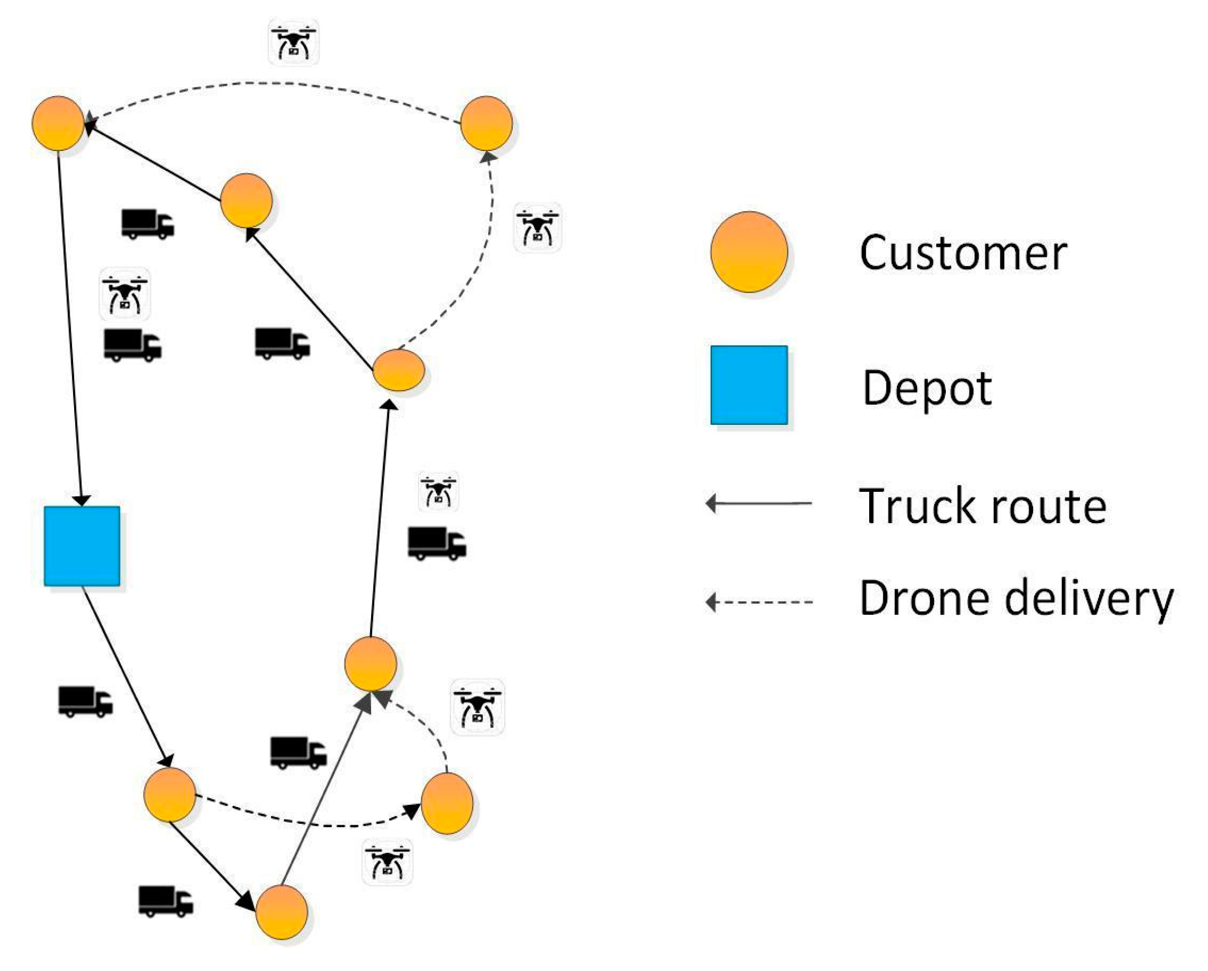
3. Problem Description and Mathematical Model

Figure 1 provides a visual illustration of a solution to the flying sidekick traveling salesman problem. The sets and parameters used in the mathematical model are also described as follows. A truck and a drone work in coordination to fulfill the demand of customers. The drone is launched from and retrieved at the depot or any one of the customer sites. The demand of each customer is a package. Let $C=\left\{1, 2, \dots , c\right\}$ be the set of all customers and $C\prime \subseteq C$ be the subset of $C$ containing all the customers that the drone can service. Although there is only one depot, for modeling purposes we use 0 and $c+1$ to represent the starting depot and ending depot, respectively. Let $N=\{0, 1, \dots , c+1\}$ be the set of all nodes; we define $N_0=\{0, 1, \dots , c\}$ and $N_{+}=\{1, 2, \dots , c+1\}$. Let ${\mathsf{\tau }}_{ij}$ be the travel time of the truck from node i to node j and ${\mathsf{\tau }}_{ij}^{\prime }$ be the travel time of the drone from node i to node j. Let $S_L$ and $S_R$ be the launching time and retrieving time of the drone and e be the endurance of the drone. P is the set of all feasible drone routes. Each element of P is denoted by a triplet $<i,j,k>$, where i, j, and k represent the launching point, customer site, and rendezvous point, respectively. A feasible route of the drone must satisfy the following three conditions:

(1)

The drone cannot be launched from the ending depot.

(2)

Each delivery point must be drone-eligible and not the drone’s launching point.

(3)

Each rendezvous point must be either the ending depot or a customer site, and the travel time of the drone should be within its endurance.

The assumptions of the FSTSP are as follows.

(1)

The drone can carry at most one package on each trip.

(2)

The drone can perform multiple delivery trips.

(3)

The truck performs at most one route.

(4)

The distance metric is the same for the truck and the drone. More specifically, both the truck and the drone travel between nodes via the street network.

(5)

The time needed to dispatch the drone from the truck is S_L (for loading a package and replacing the battery).

(6)

The time needed for the truck to receive the drone is S_R.

(7)

The drone can be dispatched or received only at the depot and customer nodes.

(8)

Both the truck and the drone must wait for the other if it first arrives at the rendezvous point (a customer site or depot). Receiving time S_R and waiting time are included in the flying time.

(9)

When the drone is dispatched from the depot, it does not need the preparation time S_L. The drone can be dispatched after the truck has left the depot.

(10)

Every customer is serviced exactly once either by the drone or the truck.

This study modifies the mathematical programming model of Murray and Chu [26] for a more compact and efficient model. The sets and parameters used in the mathematical model are also described at the beginning of this section. The modified mathematical model is as follows.

• Decision Variables

$x_{i,j}$	Binary variable. 1 if the truck travels from node i to node j; 0 otherwise.
$y_{i,j,k}$	Binary variable. 1 if the drone is dispatched at node $i$, flies from node i to node $j$, and then returns to node $k$; 0 otherwise.
$t_i$	Arrival time of the truck at node $i$.
$t_i^{\prime }$	Arrival time of the drone at node $i$.
$q_{i,j}$	Load of the truck when it traverses arc $\left(i,j\right)\in E$.
$p_{i,j}$	Auxiliary binary decision variable that equals 1 if $t_i<t_j;p_{i,j}=1$ for every $i$.
$TC$	Completion time.

• Objective Function

Minimize TC

• Constraints

$${\displaystyle \sum _{w\in M}{\displaystyle \sum _{\begin{array}{c}i\in N_0\\ i\ne j\end{array}}{x}_{{}_{i,j}}^{}}}+{\displaystyle \sum _{w\in M}{\displaystyle \sum _{\begin{array}{c}i\in N_0\\ i\ne j\end{array}}{\displaystyle \sum _{\begin{array}{c}k\in N_{+}\\ i\ne j\end{array}}{y}_{{}_{i,j,k}}^{}}}}=1 \forall j\in C$$

(1)

$${\displaystyle \sum _{j\in N_{+}}{x}_{{}_{0,j}}^{}}=1$$

(2)

$${\displaystyle \sum _{j\in N_0}{x}_{{}_{j,c+1}}^{}}=1$$

(3)

$${\displaystyle \sum _{\begin{array}{c}k\in N_{{}^{+}}\\ \langle i,j,k\rangle \in P\end{array}}{y}_{{}_{0,j,k}}^{}}\le 1 \forall j\in C$$

(4)

$${\displaystyle \sum _{\begin{array}{c}i\in N_0\\ \langle i,j,k\rangle \in P\end{array}}{y}_{{}_{i,j,c+1}}^{}}\le 1 \forall j\in C$$

(5)

$${\displaystyle \sum _{i\in N_0,k\ne j}{x}_{{}_{i,j}}^{}}={\displaystyle \sum _{k\in N^{+},k\ne j}{x}_{{}_{j,k}}^{}} \forall j\in C$$

(6)

$$2y_{i,j,k}^{}\le {\displaystyle \sum _{\begin{array}{c}h\in N_0\\ h\ne i\end{array}}{x}_{h,i}^{}+{\displaystyle \sum _{\begin{array}{c}l\in C\\ l\ne k\end{array}}{x}_{l,k}^{}}} \begin{array}{l}\forall i,j\in C,j\ne i,\\ k\in N_{+}, \langle i,j,k\rangle \in P\end{array}$$

(7)

$$y_{0,j,k}^{}\le {\displaystyle \sum _{\begin{array}{c}h\in N_0\\ h\ne k\end{array}}{x}_{h,k}^{}} \forall j\in C,k\in N_{+},\langle 0,j,k\rangle \in P$$

(8)

$$\left|N\right|x_{j,i}^{}\ge q_{j,i}^{} \forall i\in C,\forall j\in N_0$$

(9)

$${\displaystyle \sum _{j\in N_0,i\ne j}{q}_{j,i}^{}}-{\displaystyle \sum _{j\in C,i\ne j}{q}_{i,j}^{}}={\displaystyle \sum _{k\in N_0}{x}_{k,i}^{}}+{\displaystyle \sum _{\begin{array}{c}j\in C\\ j\ne i\end{array}}{\displaystyle \sum _{\begin{array}{c}k\in N_{+}\\ \langle i,j,k\rangle \in P\end{array}}{y}_{{}_{ijk}}^{}}} \forall i\in C$$

(10)

$$t_i^{\prime }\ge t_i-L(1-{\displaystyle \sum _{\begin{array}{c}j\in C\\ j\ne i\end{array}}{\displaystyle \sum _{\begin{array}{c}k\in N_{+}\\ \langle i,j,k\rangle \in P\end{array}}{y}_{i,j,k}^{})}} \forall i\in C$$

(11)

$$t_i^{\prime }\le t_i+L(1-{\displaystyle \sum _{\begin{array}{c}j\in C\\ j\ne i\end{array}}{\displaystyle \sum _{\begin{array}{c}k\in N_{+}\\ \langle i,j,k\rangle \in P\end{array}}{y}_{i,j,k}^{})}} \forall i\in C$$

(12)

$$t_k^{\prime }\ge t_k-L(1-{\displaystyle \sum _{\begin{array}{c}i\in N_0\\ i\ne k\end{array}}{\displaystyle \sum _{\begin{array}{c}j\in C\\ \langle i,j,k\rangle \in P\end{array}}{y}_{i,j,k}^{})}} \forall k\in N_{+}$$

(13)

$$t_k^{\prime }\le t_k+L(1-{\displaystyle \sum _{\begin{array}{c}i\in N_0\\ i\ne k\end{array}}{\displaystyle \sum _{\begin{array}{c}j\in C\\ \langle i,j,k\rangle \in P\end{array}}{y}_{i,j,k}^{})}} \forall k\in N_{+}$$

(14)

$$\begin{array}{c}{t}_k\ge t_h+{\mathsf{\tau }}_{hk}+s_L({\displaystyle \sum _{\begin{array}{c}l\in C\\ l\ne k\end{array}}{\displaystyle \sum _{\begin{array}{c}m\in N_{+}\\ \langle k,l,m\rangle \in P\end{array}}{y}_{{}_{k,l,m}}^{})+}}\\ s_R({\displaystyle \sum _{\begin{array}{c}i\in N_0\\ i\ne k\end{array}}{\displaystyle \sum _{\begin{array}{c}j\in C\\ \langle i,j,k\rangle \in P\end{array}}{y}_{{}_{i,j,k}}^{})-L(1-x_{{}_{hk}}^{})}}\end{array} \forall h\in N_0,k\in N_{+},k\ne h$$

(15)

$$t_j^{\prime }\ge t_i^{\prime }+{\mathsf{\tau }}_{ij}^{\prime }-L(1-{\displaystyle \sum _{\begin{array}{c}k\in N_{+}\\ \langle i,j,k\rangle \in P\end{array}}{y}_{i,j,k}^{}}) \forall j\in C\prime , i\in N_0, i\ne j$$

(16)

$$t_k^{\prime }\ge t_j^{\prime }+{\mathsf{\tau }}_{jk}^{\prime }+S_R-L(1-{\displaystyle \sum _{\begin{array}{c}i\in N_0\\ \langle i,j,k\rangle \in P\end{array}}{y}_{i,j,k}^{}}) \forall j\in C\prime , k\in N_{+},k\ne j$$

(17)

$$t_k^{\prime }-t_i^{\prime }-S_L({\displaystyle \sum _{\begin{array}{c}z\in C\\ \langle k,z,m\rangle \in P\end{array}}{y}_{k,z,m}^{})}\le e+L(1-y_{i,j,k}^{}) \begin{array}{c}\forall k\in N_{+},j\in C,j\ne k,\\ i\in N, \langle i,j,k\rangle \in P\end{array}$$

(18)

$$t_i^{}+{\mathsf{\tau }}_{i,c+1}{x}_{i,c+1}\le TC \forall i\in N$$

(19)

$$t_{c+1}^{\prime }\le TC$$

(20)

$$p_{ij}+p_{ji}=1 \forall i,j\in C,j\ne i$$

(21)

$$x_{{}_{i,j}}^{}\le p_{ij} \forall i\in N_0,j\in N_{{}^{+}},j\ne i$$

(22)

$$t_l^{\prime }\ge t_k^{\prime }-L\left(3-{\displaystyle \sum _{\begin{array}{c}j\in C\\ j\ne l\\ \langle i,j,k\rangle \in P\end{array}}{y}_{i,j,k}^{}-{\displaystyle \sum _{\begin{array}{c}m\in C\\ m\ne i\\ m\ne k\\ m\ne l\end{array}}{\displaystyle \sum _{\begin{array}{c}n\in C\\ j\ne l\\ \langle i,j,k\rangle \in P\end{array}}{y}_{l,m,n}^{}}}}-P_{il}\right) \begin{array}{l}\forall i\in N_0,k\in N_{+}, k\ne i, \\ l\in C,l\ne i,l\ne k\end{array}$$

(23)

$$t_{0,i}^{}=0, \forall i\in C$$

(24)

$$t_i^{}\ge 0, t{\prime }_i\ge 0, q_{i,j}^{}\ge 0 \forall i\in N_{+},j\in C,j\ne k$$

(25)

$$x_{i,j}^{},p_{i,j}^{},y_{{}_{i,j,k}}^{}\in \{0,1\}$$

(26)

Constraint (1) confirms that the drone or the truck services every customer once precisely. Constraints (2) and (3) guarantee the departure and the return of the truck from and to the depot. Constraints (4) and (5) restrict the drone from being dispatched from the depot at most once and returns to the depot at most once. Constraint (6) is the flow conservation constraint for the truck. Constraint (7) ensures that if the drone is dispatched from node i and received at node k, then the truck visits both nodes i and k. Constraint (8) makes sure that if the drone is dispatched from the depot and received at node k, then the truck visits node k. Constraint (9) is the capacity constraint. Constraint (10) forbids sub-tours.

Constraints (11) and (12) synchronize the time between the truck and the drone. When the drone is dispatched from the truck at a customer node, say, i, the departure times of the drone and the truck at node i must be the same. However, the drone and the truck may depart from the depot separately. Similarly, constraints (13) and (14) also synchronize the time between the truck and the drone. If the drone is received at a customer node, say, k, then the drone and the truck arrive at node k simultaneously. Note that constraints (11)–(14) ensure that the drone cannot be received at the node where it was dispatched. Moreover, it cannot be dispatched from a node multiple times.

Constraint (15) ensures that if the truck travels from node h to node k, its effective arrival time at node k must include the arrival time at node h and the travel time from node h to node k. Constraint (16) states that if the drone is launched from node i, its arrival time at any other node, say, j, must include the travel time from node i to node j. Likewise, constraint (17) ensures that if the drone is retrieved at a node, say, k, the truck’s arrival time at node k must include its travel time from node j to node k and the recovery time $S_R$. Constraint (18) ensures that the operation time of the drone is within its endurance.

Constraint (19) states that the completion time should be no earlier than the truck’s arrival at the depot. Similarly, constraint (20) states that the completion time should be no earlier than the drone’s arrival at the depot. Constraints (21) and (22) determine the precedence relationship between each pair of customers. Constraint (23) guarantees that if the drone is dispatched from node l and received at node k, then its launch time from l, $t_{w,l}^{\prime }$ does not precede its return time to k, $t_{w,k}^{\prime }$. Also, this constraint will not bind if the drone is not launched from l or does not return to k, or if i does not precede l. Constraint (24) determines the departure time of the truck at the depot. Constraints (25) and (26) are variable constraints.

Our mathematical model uses truckload constraints (9) and (10) to avoid sub-tours in the truck route, as opposed to using constraints (5), (11), (20), and (21) found in the work of Murray and Chu [26]. This modification renders our model more compact and more efficient. Specifically, the total number of constraints in our model, comprising constraints (9) and (10), is |C| × |N₀| + |C|. In contrast, the total number of constraints (5), (11), (20), and (21) used in Murray and Chu [26] is 2 × |C| × (|N₊| − 1) + 2 × |C| × (|C| − 1).

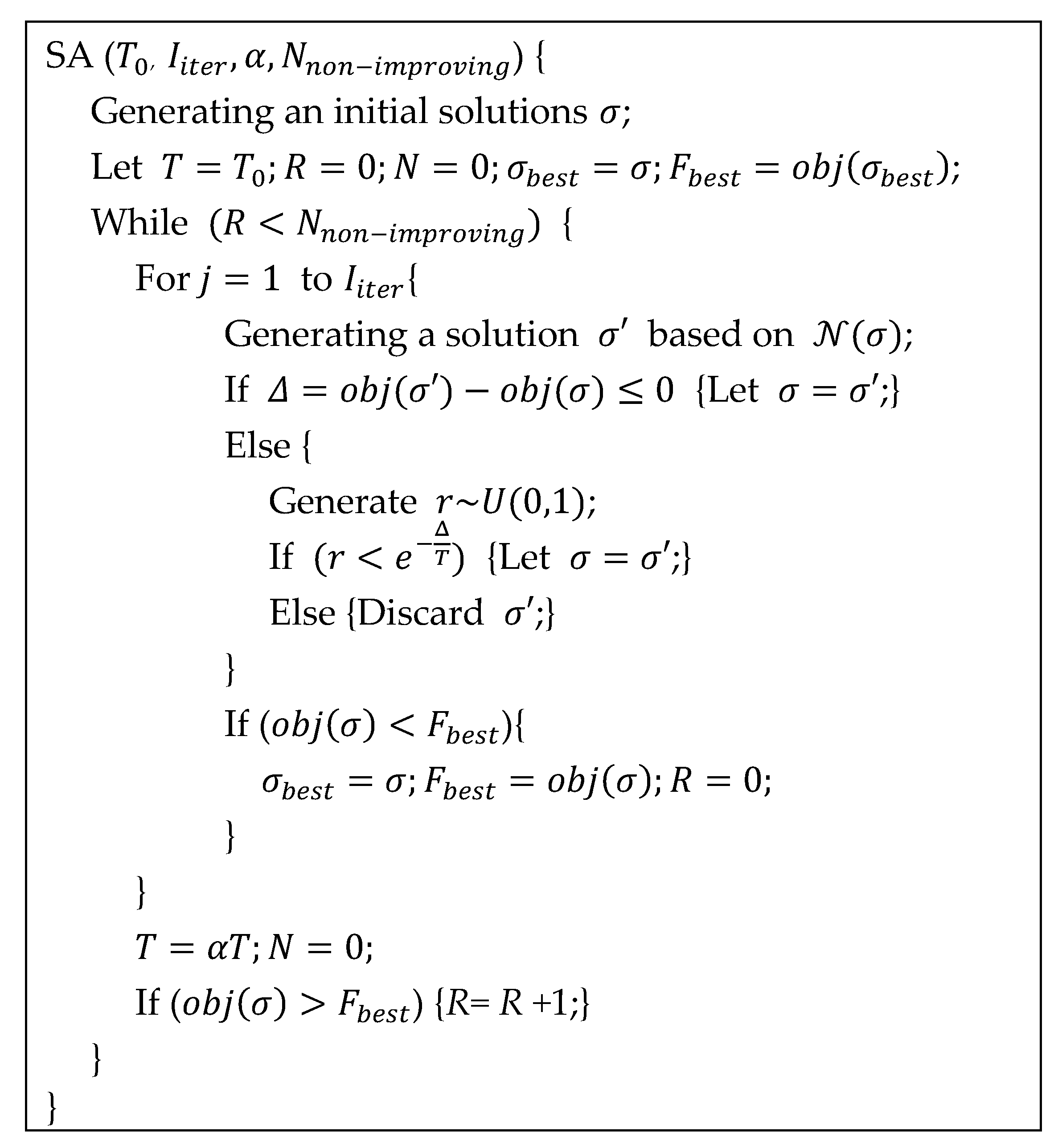
4. Simulated Annealing Heuristic for the FSTSP

This study develops a simulated annealing heuristic for solving the FSTSP. SA is chosen mainly due to its effectiveness and simplicity. Kirkpatrick et al. [47] introduced SA based on the algorithm developed by Metropolis et al. [48]. Several complex combinatorial analyses and real-world problems are solved by the heuristic [49,50,51,52,53,54,55].

An initial solution is randomly generated to begin the SA. A new neighborhood solution is subsequently chosen to replace the current solution if its objective function value is better than that of the current one at each iteration. A solution with a worse objective function value may also be accepted as the new solution, with a small probability to allow the search to move to worse solutions, and thus enables SA to escape from local optimum. The following subsections further discuss the solution representation, initial solution, neighborhood, and SA procedure for solving the FSTSP.

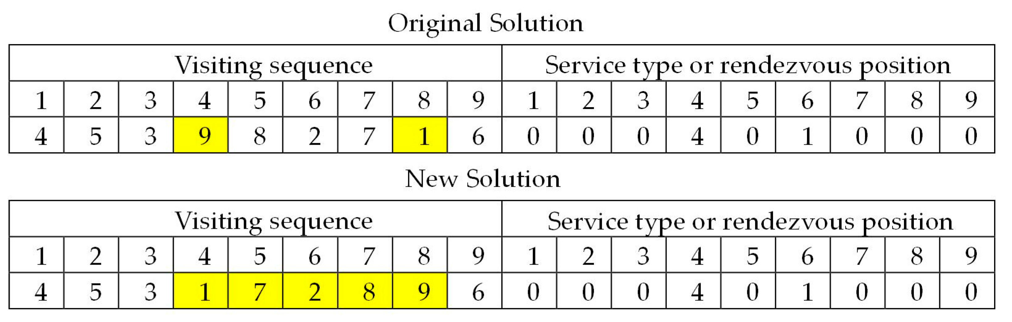
4.1. Solution Representation

A FSTSP solution is divided into two parts. The first part is a permutation of c customers, denoted by the set $\{1, 2, \dots , c\}$, in which the jth number indicates the jth customers to be serviced. The second part indicates the service type (vehicle or drone) of individual customers ranging from 0 to $c-1$, where c denotes the number of customers. If a customer is serviced by the vehicle, the service type is set as 0. Otherwise, the service type is set to be the number of customers serviced by the truck between the sortie of the drone and the rendezvous, say, r. If the number of remaining customers to be serviced by the vehicle after launching the drone at a customer is smaller than r, the rendezvous of this customer is set to be a depot. The service type of some customers will be changed to zero if (1) they cannot be serviced by drone as the constraints imposed; (2) the drone is not in the vehicle; (3) the rendezvous cannot receive the drone; and (4) the flying distance (from the launching node to the customer and coming back to the rendezvous) exceeds the endurance of the drone.

4.2. Illustration of Solution Representation

Two graphic examples from Murray and Chu [26] are used to demonstrate the proposed solution representation. There are nine customers in both examples. The graphic example of Figure 9b in Murray and Chu [26] can be encoded by the solution representation shown in Figure 2. By scanning the visiting sequence in the first part, and choosing only the customers with service type zero, the visiting sequence of the vehicle is obtained as 5-3-9-8-2-7-1. Because the service type (or rendezvous position) of customer four is four and it is the first customer to be serviced, the drone is launched from the depot, and the rendezvous position is customer eight (the fourth customer to be serviced by the vehicle after customer four). Since the vehicle services customer one last, it will return to the depot after leaving customer one. Because the service type (or rendezvous position) of customer six is one and its previous truck customer is customer one, the drone will be launched at customer one, fly to customer six and then go back to the depot. It should be noted that if the service type of a drone customer is changed to zero, the route of the vehicle will change. Furthermore, if the drone is launched or received by the vehicle, the launching time (S_L) and the receiving time (S_R) should be included in calculating the traveling time of the vehicle.

The second graphic example in Figure 10b of Murray and Chu [26] is encoded by the solution representation shown in Figure 3. In a similar way, the visiting sequence of the vehicle is obtained as 3-9-8-2-7-6-1. The drone is launching from the depot to service customer five first since this customer is the first to be serviced. The rendezvous position of customer five is one, so the rendezvous position is customer three (the first customer to be serviced by a vehicle after the drone is launched). Because the service type (or rendezvous position) of customer four is three and the first truck customer before customer four is customer eight, the drone will be launched at customer eight to service customer four, and then be received at customer six (the third customer to be serviced by vehicle after customer eight).

4.3. Neighborhood

Let $\mathsf{\sigma }$ represent the current solution, and $N(\mathsf{\sigma })$ denote the set of solutions in the neighborhood of $\mathsf{\sigma }$. $N(\mathsf{\sigma })$ is generated by either one of the swap, insertion, inversion, and change in service type operators. The swap operator switches the positions of two randomly selected elements in the first part of $\mathsf{\sigma }$. The insertion operator inserts a random element immediately before another random element in the first part of $\mathsf{\sigma }.$ The inversion operator reverses the order of a random substring in the first part of $\mathsf{\sigma }.$ The change of service type operator randomly chooses an element in the second part of $\mathsf{\sigma }$ and changes its value at random (between 0 and $N-1$). The four operators are illustrated in Figure 4, Figure 5, Figure 6 and Figure 7. The probabilities of performing the swap, insertion, inversion, and change in the service type operators are fixed at 0.25, 0.25, 0.25, and 0.25, respectively.

4.4. Parameter Setting and the SA Procedure

Initially, $T_0$ stands as the present temperature $T$ and $\mathsf{\sigma }$ is the random initial solution. $\mathsf{\sigma }$ consists of a random service sequence of $N$ customers and $N$ service types. ${\mathsf{\sigma }}_{best}$ represents the current best solution and $F_{best}$ denotes the current best objective function value, $obj(\mathsf{\sigma })$. The objective function is the completion time. The calculation of the completion time can be referred to as the MILP of the FSTSP as proposed by Murray and Chu [26]. The algorithm searches the neighborhood of $\mathsf{\sigma }$, $N(\mathsf{\sigma })$, to obtain a new solution ${\mathsf{\sigma }}^{\prime }$ with the objective function value $obj\left({\mathsf{\sigma }}^{\prime }\right)$. Let $\mathsf{\Delta }=obj\left({\mathsf{\sigma }}^{\prime }\right)-obj(\mathsf{\sigma })$ be the change in the objective function value. If $\mathsf{\Delta }<0$ (i.e., ${\mathsf{\sigma }}^{\prime }$ is better than $\mathsf{\sigma }$), then $\mathsf{\sigma }$ is replaced by $\mathsf{\sigma }$. Otherwise, the algorithm replaces $\mathsf{\sigma }$ by $\mathsf{\sigma }\prime$ with the probability $e^{-\mathsf{\Delta }/T}$. The best solution obtained so far and its objective function value, ${\mathsf{\sigma }}_{best}$ and $F_{best}$, are continuously updated as the algorithm proceeds.

The current temperature $T$ decreases after $I_{iter}$ iterations at the rate of $T=\mathsf{\alpha }T$, $0<\mathsf{\alpha }<1$. The algorithm stops when ${\mathsf{\sigma }}_{best}$ is unchanged after the $N_{non-improving}$ consecutive temperature decreases. Finally, the algorithm derives the best FSTSP solution from ${\mathsf{\sigma }}_{best}$. Figure 8 depicts the pseudocode of the proposed SA heuristic.

5. Experimental Results

This section presents the comparative results of the proposed solution approaches (SA and modified MILP), several heuristics (IP, Saving, Nearest neighbor, and Sweep), and MILP of Murray and Chu [26] for the FSTSP. Furthermore, the proposed SA is compared with the state-of-the-art algorithms HGA [34] and ILS [35] for the FSTSP. An Intel^® Xeon^® E3-1245 v6@ 3.7 GHz computer with 64 GB of RAM is used to test the proposed SA in C++. The following subsections explain the test problems, parameter selection, and experimental results.

5.1. Test Problems

Two FSTSP benchmark datasets are used to verify the performance of the proposed simulated annealing heuristic. The first dataset is taken from Murray and Chu [26]. The second dataset is adopted from Ha, Deville, Pham, and Hà [33]. The characteristics of the two datasets are briefly described below.

The first FSTSP benchmark dataset includes 72 instances. Each instance has ten customers distributed over an eight-mile square region. The depot of each instance is set at random. It is either the origin (southwest corner of the area), the center of gravity, or the average x-coordinate of customers, 0. UAV-eligible customers are randomly set and comprise 80–90% of the total population. Twenty or forty minutes is randomly assigned to be the endurance of the UAV. The speed of the UAV is set to be 15, 25, or 35 miles per hour at random based on Euclidean UAV flight paths. The speed of the truck is set as 25 miles/h. The truck route is based on the Manhattan metric. Both SL and SR are set to be one minute. In addition, the Euclidean distance between customers corresponds to the traveling time between customers for the UAV.

The second FSTSP benchmark dataset contains 60 instances. In each instance, there are either 50 or 100 customers whose locations are generated at random in a square region of 100 km², 500 km², or 1000 km². Manhattan distance is used for the truck, while Euclidean distance is used for the drone to reflect the difference in the ways the truck and the drone travel. The truck and the drone travel at the same speed of 40 km/h. The endurance or flight time of the drone is 20 min.

The depot location is set at the lower left corner of the entire service area. For every instance, only 80% of the customers can be serviced by drone to reflect the real situation. As in Murray and Chu [26], both the start time S_L and pickup time S_R are 1 min.

5.2. Parameter Selection

$T_0$, $I_{iter}$, $\mathsf{\alpha }$, and $N_{non-improving}$ are the four parameters used in the proposed SA, where $T_0$ denotes the initial temperature, $I_{iter}$ represents the number of iterations to be performed at a particular temperature, $\mathsf{\alpha }$ is the cooling rate, and $N_{non-improving}$ is the maximum number of consecutive temperature reductions during which the best objective function value has not been improved. In the following, we will show how the parameter values are determined.

The parameter values have 4⁴ combinations since each of the four parameters has four levels, as shown in

Table 1. Orthogonal array and the obtained ARPDs for the FSTSP.

Experiment No.	${\mathit{T}}_0$	${\mathit{I}}_{\mathit{i}\mathit{t}\mathit{e}\mathit{r}}$	$\mathit{\alpha }$	${\mathit{N}}_{\mathit{n}\mathit{o}\mathit{n}-\mathit{i}\mathit{m}\mathit{p}\mathit{r}\mathit{o}\mathit{v}\mathit{i}\mathit{n}\mathit{g}}$	ARPD for FSTSP
1	1.0	5000 L *	0.900	5	1.0586
2	1.0	10,000 L	0.925	10	0.8969
3	1.0	15,000 L	0.950	15	0.8168
4	1.0	20,000 L	0.975	20	0.7168
5	1.5	5000 L	0.925	15	0.8259
6	1.5	10,000 L	0.900	20	0.8041
7	1.5	15,000 L	0.975	5	0.7427
8	1.5	20,000 L	0.950	10	0.6790
9	2.0	5000 L	0.950	20	0.7698
10	2.0	10,000 L	0.975	15	0.7032
11	2.0	15,000 L	0.900	10	0.7255
12	2.0	20,000 L	0.925	5	0.7428
13	2.5	5000 L	0.975	10	0.8806
14	2.5	10,000 L	0.950	5	0.8466
15	2.5	15,000 L	0.925	20	0.6737
16	2.5	20,000 L	0.900	15	0.7009

*: $L$ Denotes the length of solution representation.

. To determine the best values of the four parameters in combination more effectively, the Taguchi L16 orthogonal design of the experiment that has 16 parameter combinations obtained by PASS 2023 software (https://www.ncss.com/software/pass/) (accessed on 1 August 2023) is applied to six randomly generated test instances for the FSTSP. The proposed SA algorithm is used to solve each of the selected instances 30 times independently. Table 1 exhibits the average relative percentage deviation (ARPD) of the best solutions obtained by using different levels of the parameters. The ARPD is computed as $\mathrm{A}\mathrm{R}\mathrm{P}\mathrm{D}=\frac{{\sum }_{i=1}^6{\sum }_{j=1}^{30}\left(ob{j}_{ij}-ob{j}_i^{best}\right)}{ob{j}_i^{best}}\times 100\%$, where $O{bj}_{ij}$ denotes the total distance of the solution obtained in the jth ($j=1, \dots , 30$) replicate of test instance $i (i=1, \dots , 6)$ using the SA algorithm with a designated parameter combination; $ob{j}_i^{best}$ is the total distance of the best solution obtained among 30 replicates of test instance $i (i=1, \dots , 6)$ using the SA algorithm with a designated parameter combination.

Table 2. ARPDs obtained by different levels of each parameter for the FSTSP.

Level	${\mathit{T}}_0$	${\mathit{I}}_{\mathit{i}\mathit{t}\mathit{e}\mathit{r}}$	$\mathit{\alpha }$	${\mathit{N}}_{\mathit{n}\mathit{o}\mathit{n}-\mathit{i}\mathit{m}\mathit{p}\mathit{r}\mathit{o}\mathit{v}\mathit{i}\mathit{n}\mathit{g}}$
1	0.8723	0.8837	0.8223	0.8477
2	0.7629	0.8127	0.7848	0.7955
3	0.7353	0.7396	0.7780	0.7617
4	0.7754	0.7099	0.7608	0.7411
Range	0.1369	0.1739	0.0615	0.1066
Rank	2	1	4	3

displays the statistical significance for the FSTSP. $I_{iter}$ has the largest range of ARPD and is the most significant among the four parameters. In addition, the proposed SA algorithm can produce a better solution in a prolonged process, as more solutions are evaluated at the same temperature. $T_0, I_{iter}, \mathsf{\alpha },$ and $N_{non-improving}$ are set to be 2.0, 20,000 L, 0.975, and 20, respectively, when solving the FSTSP instances to seek a balance between the solution time and solution quality.

5.3. Results and Discussion

It should be noted that the several heuristics (IP, Savings, Nearest neighbor, and Sweep) proposed by Murray and Chu [26] were run on a PC with an Intel quad-core i7–860 processor and 4 GB RAM under 64-bit Ubuntu Linux 14.04 [26], which is different from the computer used in this study. Since the hardware, software, and code efficiency all affect solution time, a direct comparison between the efficiency of the algorithms is infeasible. Therefore, the single-thread performance of CPUs (http://www.cpubenchmark.net/singleThread.html, accessed on 1 August 2023) is used to measure the relative speed of different processors. The original computer used to run the several heuristics (IP, Saving, Nearest neighbor, and Sweep) has a score of 1319. The computer running the proposed SA heuristic has a score of 2429. The HGA and ILS are implemented in C++ and compiled with the “−O3” flag. The experiments are run on a desktop computer with an Intel Core i7-6700, 3.4 GHz processor which has a score of 2302. The speed of the computer for the HGA and ILS are similar to the speed of the computer used by the proposed SA. Because the HGA and ILS are executed 10 times for the first FSTSP dataset, the proposed SA is also executed 10 times and the best and average solutions among 10 runs are recorded for comparison. Because the MILP_MC used the same maximal computational time (1800 s), the maximal computational time is set to 1800 s to MILP_New.

The objective function values of the best solutions for each benchmark instance obtained using various algorithms are compared based on the relative percentage deviation (RPD), calculated as

$${\mathrm{RPD}}_h=\frac{Ob{j}_h^{}-Ob{j}_B^{}}{Ob{j}_B^{}}\times 100\%,$$

where $Ob{j}_h$ and $Ob{j}_B$ are the best objective function values obtained by solution approach h and the best-known solution (BKS), respectively.

Table 3. Summary of results obtained by various solution approaches for the first FSTSP dataset.

Method	Average RDP for the Best Solution among 10 Runs	Max. RDP for 72 Benchmark Problems	# of BKS Attained
IP	2.072%	14.083%	32
Savings !	3.604%	18.300%	21
Nearest !	6.215%	21.315%	12
Sweep	11.807%	36.803%	1
HGA	0.008%	0.569%	71
ILS	0.000%	0.000%	72
SA	0.000%	0.000%	72
MILPMC	0.000%	30.486%	31
MILPNew	0.000%	4.186%	57

! Incorrect solutions are excluded.

summarizes results obtained by the various heuristics compared for the first FSTSP dataset. The detailed objective function values obtained by these solution approaches are listed in

Table 4. The objective function values obtained by various heuristics on the FSTSP for the first problem dataset.

No.	IP	Savings	Nearest	Sweep	HGA	ILS	SA	MILPMC	MILPnew	No.	IP	Savings	Nearest	Sweep	HGA	ILS	SA	MILPMC	MILPnew
1	56.468	56.709	57.992	57.992	56.468	56.468	56.468	56.468	56.468	37	49.996	49.996	50.030	58.378	49.422	49.422	49.422	51.922	49.422
2	50.573	50.813	52.625	52.096	50.573	50.573	50.573	52.096	52.690	38	49.470	49.470	49.470	54.493	49.204	49.204	49.204	49.204	49.204
3	53.207	55.351	53.207	57.367	53.207	53.207	53.207	53.207	53.207	39	62.796	62.796	64.270	69.147	62.576	62.222	62.222	65.624	62.222
4	47.311	53.761	47.311	51.471	47.311	47.311	47.311	47.311	47.311	40	62.270	62.270	62.270	68.183	62.004	62.004	62.004	62.270	62.004
5	53.687	53.687	53.687	56.395	53.687	53.687	53.687	53.687	53.687	41	42.799	46.367	51.599	44.253	42.533	42.533	42.533	44.253	42.799
6	53.687	53.687	53.687	56.241	53.687	53.687	53.687	53.687	54.241	42	42.799	46.367	50.015	44.253	42.533	42.533	42.533	44.253	42.799
7	67.464	67.464	67.464	80.958	67.464	67.464	67.464	67.464	67.464	43	43.342	43.342	43.369	52.503	43.076	43.076	43.076	43.076	43.076
8	66.487	66.487	66.487	80.726	66.487	66.487	66.487	66.487	66.487	44	43.342	43.342	43.369	52.503	43.076	43.076	43.076	43.076	43.297
9	51.149	51.390	51.172	51.172	50.551	50.551	50.551	50.551	51.634	45	49.204	49.204	49.470	56.347	49.204	49.204	49.204	49.204	49.204
10	51.149	51.149	51.149	51.149	44.835	44.835	44.835	45.835	44.835	46	49.204	49.204	49.470	54.423	49.204	49.204	49.204	49.204	49.204
11	45.176 !	47.601	45.176 !	46.576	47.311	47.311	47.311	47.601	47.601	47	62.004	62.004	64.270	69.881	62.004	62.004	62.004	62.004	62.004
12	45.863	47.601	45.863	46.576	43.602	43.602	43.602	47.601	44.285	48	62.004	62.004	62.830	64.404	62.004	62.004	62.004	62.004	62.004
13	49.581	49.581	49.581	49.581	49.581	49.581	49.581	51.887	49.581	49	69.586	69.586	82.280	79.760	69.586	69.586	69.586	69.586	69.586
14	47.791	47.791	47.791	48.369	46.621	46.621	46.621	46.621	46.621	50	55.493	55.493	59.413	57.251	55.493	55.493	55.493	57.251	55.493
15	62.381	62.381	62.381	75.983	62.381	62.381	62.381	64.687	62.381	51	72.146	74.740	86.043	86.605	72.146	72.146	72.146	72.146	72.146
16	60.591	60.591	60.591	69.247	59.416	59.416	59.416	59.776	59.416	52	58.053	58.053	64.054	76.009	58.053	58.053	58.053	58.053	58.053
17	46.254	46.254	46.276	46.276	42.416	42.416	42.416	45.985	42.996	53	77.344	82.083	91.763	91.304	77.344	77.344	77.344	77.344	77.344
18	46.254	46.254	46.254	46.254	42.416	42.416	42.416	42.416	42.416	54	69.900	70.853	74.773	74.454	68.431	68.431	68.431	69.175	69.431
19	42.416	47.601	42.416	46.576	41.729	41.729	41.729	43.093	41.729	55	90.144	94.883	104.563	105.104	90.144	90.144	90.144	90.144	90.144
20	42.416	47.601	42.416	46.576	41.729	41.729	41.729	41.729	41.729	56	82.700	83.653	89.654	88.947	82.700	82.700	82.700	82.700	82.700
21	42.896	42.896	42.896	48.369	42.896	42.896	42.896	48.214	42.896	57	55.493	55.493	61.707	57.251	54.973	54.973	54.973	63.247	55.302
22	42.896	42.896	42.896	48.369	42.896	42.896	42.896	42.896	42.896	58	53.980	53.980	54.252	53.741	51.929	51.929	51.929	53.447	52.093
23	56.696	56.696	56.696	76.983	56.273	56.273	56.273	61.569	56.273	59	58.053	60.530	64.054	64.054	55.209	55.209	55.209	64.702	55.209
24	55.696	55.696	55.696	59.653	55.696	55.696	55.696	55.696	55.696	60	57.088	57.088	53.837	60.249	52.329	52.329	52.329	52.329	52.329
25	49.430	53.890	55.111	53.044	49.430	49.430	49.430	49.430	49.430	61	69.009	64.409 !	68.489	70.650	65.523	65.523	65.523	67.770	65.523
26	46.886	48.340	54.952	48.340	46.886	46.886	46.886	48.723	46.886	62	64.841	64.409	65.010	65.105	60.743	60.743	60.743	60.743	61.886
27	50.708	52.133	57.591	58.628	50.708	50.708	50.708	50.708	50.708	63	80.809	77.209 !	81.289	86.777	78.323	78.323	78.323	83.700	78.323
28	46.423	46.423	47.543	58.582	46.423	46.423	46.423	46.423	46.423	64	74.686	73.967	77.209	80.809	72.967	72.967	72.967	74.686	74.686
29	56.102	56.102	62.331	71.426	56.102	56.102	56.102	56.102	56.102	65	49.049	49.049	54.658	50.009	45.931	45.931	45.931	59.321	45.931
30	56.102	56.102	57.060	57.102	53.933	53.933	53.933	53.933	55.223	66	49.049	49.049	54.658	50.009	45.931	45.931	45.931	47.250	46.740
31	69.902	69.902	76.131	81.606	69.902	69.902	69.902	69.902	69.902	67	47.935	55.524	54.481	64.155	46.935	46.935	46.935	61.240	47.935
32	68.902	68.902	74.717	71.757	68.397	68.397	68.397	68.397	68.902	68	47.935	53.555	52.481	60.249	46.935	46.935	46.935	48.865	47.935
33	43.533	49.787	45.950	44.987	43.533	43.533	43.533	45.358	43.533	69	61.886	57.382	60.476	60.744	56.395	56.395	56.395	67.435	56.395
34	43.533	46.358	50.979	44.987	43.533	43.533	43.533	46.590	43.533	70	61.886	57.382	57.265	60.744	56.395	56.395	56.395	56.395	57.382
35	44.076	44.076	45.040	50.876	43.949	56.468	43.949	44.076	44.076	71	74.686	69.195	73.276	75.436	69.195	69.195	69.195	83.700	69.195
36	44.076	44.076	44.076	47.900	43.810	50.573	43.810	44.076	43.810	72	73.894	69.195	69.195	80.809	69.195	69.195	69.195	69.195	69.195

A bold number indicates the best results obtained. ! denotes infeasible solutions.

. The average RPD on the best solution among 10 runs of the proposed SA heuristic is 0.000%, whereas the corresponding values for IP, Savings, Nearest, Sweep, HGA, ILS, MILP_MC, and MILP_New are 2.072%, 3.604%, 6.215%, 11.807%, 0.008%, 0.000%, 3.537%, and 0.421%, respectively. The maximal RPD on the 72 benchmark instances for the proposed SA is 0.000%, whereas the corresponding values for IP, Savings, Nearest, Sweep, HGA, and ILS are 14.083%, 18.300%, 21.315%, 36.803%, 0.569%, 0.000%, 30.486%, and 4.186%, respectively. Therefore, the proposed SA algorithm is competitive to the existing methods. It should be noted that the solutions to Problems 11, 61, and 63 reported in Murray and Chu (2015) are incorrect. For the 72 benchmark instances, the proposed SA finds 72 BKSs (72/72 = 100.00%), while IP, Savings, Nearest, Sweep, HGA, and ILS find 32 (32/72 = 44.444%), 21 (21/72 = 29.167%), 12 (12/72 = 16.667%), 1 (1/72 = 1.389%), 70 (71/72 = 98.611%), 72 (72/72 = 100.00%) BKSs, 37 (37/72 = 51.389%), and 51 (51/72 = 70.833%), respectively. Clearly, the proposed SA and ILS heuristics obtain more BKSs than any one of the other solution approaches in the comparison. Furthermore, the proposed SA requires merely 1.091 s on average and 1.775 s maximum. These results show that the proposed SA heuristic either outperforms or is comparable with state-of-the-art algorithms in solving the FSTSP.

Table 5. Summary of results obtained by various solution approaches for the second FSTSP dataset.

Method	Average RDP for the Best Solution among 10 Runs	Average RDP for the Average Solution among 10 Runs	# of BKS Obtained	Average Computing Time (Min)
HGA	0.258%	0.812%	27	2.66
ILS	0.720%	2.915%	16	1.59
SA	0.261%	1.043%	29	2.52

summarizes results obtained by the various heuristics for the second dataset. The detailed objective function values obtained by these solution approaches are listed in

Table 6. The objective function values obtained by various heuristics for the second FSTSP dataset with N = 50.

Inst.	BKS	ILS					HGA					SA
		Best	Gap	Ave.	Gap	Time (m)	Best	Gap	Ave.	Gap	Time (m)	Best	Gap	Ave.	Gap	Time (m)
B1	115.59	115.65	0.05	116.43	0.73	0.76	115.72	0.11	118.45	2.47	0.38	115.59	0.00	116.36	0.67	1.21
B2	118.39	118.39	0.00	118.39	0.00	0.33	118.39	0.00	119.96	1.33	0.36	118.39	0.00	118.88	0.41	1.07
B3	116.21	116.21	0.00	116.39	0.15	0.57	116.21	0.00	118.79	2.22	0.47	116.21	0.00	116.25	0.03	1.09
B4	118.71	118.71	0.00	119.26	0.46	0.47	118.99	0.24	120.65	1.63	0.48	118.93	0.19	119.09	0.32	1.07
B5	115.78	115.78	0.00	115.91	0.11	0.58	115.78	0.00	118.48	2.33	0.38	116.72	0.81	117.53	1.51	1.09
B6	114.31	114.31	0.00	115.46	1.01	0.88	115.26	0.83	117.97	3.20	0.46	115.11	0.70	115.96	1.44	1.08
B7	115.52	115.52	0.00	115.63	0.10	0.62	115.53	0.01	116.63	0.96	0.41	115.52	0.00	115.67	0.13	1.08
B8	117.16	117.90	0.63	118.04	0.75	0.78	117.90	0.63	118.28	0.96	0.39	117.16	0.00	118.02	0.73	1.09
B9	117.64	117.64	0.00	117.72	0.07	0.39	117.72	0.07	118.69	0.89	0.37	117.72	0.07	117.73	0.08	1.10
B10	116.94	117.38	0.38	117.70	0.65	0.60	117.74	0.68	119.13	1.87	0.44	116.94	0.00	117.75	0.69	1.08
C1	215.00	215.07	0.03	215.37	0.17	0.60	215.00	0.00	218.87	1.80	0.43	215.47	0.22	215.64	0.30	1.24
C2	208.66	209.23	0.27	210.11	0.69	0.53	209.69	0.49	210.47	0.87	0.35	208.66	0.00	209.45	0.38	1.18
C3	212.02	212.02	0.00	212.22	0.09	0.38	212.02	0.00	214.38	1.11	0.24	212.36	0.16	212.36	0.16	1.14
C4	212.00	212.08	0.04	213.27	0.60	0.60	213.45	0.68	217.67	2.67	0.44	212.00	0.00	214.85	1.34	1.26
C5	220.50	223.06	1.16	224.57	1.85	0.48	220.50	0.00	226.23	2.60	0.34	220.50	0.00	224.03	1.60	1.22
C6	233.67	234.01	0.15	235.56	0.81	0.31	233.67	0.00	237.38	1.59	0.31	233.67	0.00	235.76	0.89	1.16
C7	222.27	222.27	0.00	223.40	0.51	0.51	222.81	0.24	227.99	2.57	0.45	224.08	0.81	224.08	0.81	1.22
C8	233.43	234.26	0.36	237.53	1.76	0.46	233.71	0.12	238.45	2.15	0.39	233.43	0.00	236.89	1.48	1.19
C9	223.57	226.01	1.09	227.43	1.73	0.68	226.02	1.10	233.10	4.26	0.42	223.57	0.00	226.19	1.17	1.26
C10	225.93	226.17	0.11	226.17	0.11	0.48	225.93	0.00	229.74	1.69	0.38	226.90	0.43	226.97	0.46	1.22
D1	304.73	306.39	0.54	307.09	0.77	0.61	304.73	0.00	313.18	2.77	0.33	305.45	0.24	307.27	0.83	1.24
D2	311.56	313.93	0.76	315.64	1.31	0.57	311.80	0.08	317.17	1.80	0.35	311.56	0.00	314.03	0.79	1.24
D3	293.31	295.86	0.87	297.54	1.44	0.60	294.23	0.31	308.78	5.27	0.36	293.31	0.00	294.10	0.27	1.22
D4	323.42	323.72	0.09	324.60	0.36	0.56	323.42	0.00	329.17	1.78	0.33	324.13	0.22	326.23	0.87	1.18
D5	319.17	321.46	0.72	321.83	0.83	0.40	319.17	0.00	320.89	0.54	0.24	319.44	0.08	320.10	0.29	1.22
D6	313.11	313.21	0.03	313.65	0.17	0.49	313.11	0.00	314.13	0.33	0.28	314.03	0.29	314.99	0.60	1.18
D7	316.65	316.65	0.00	317.83	0.37	0.32	319.92	1.03	323.78	2.25	0.35	316.87	0.07	316.88	0.07	1.17
D8	289.48	293.76	1.48	296.51	2.43	0.58	289.48	0.00	292.39	1.01	0.33	289.48	0.00	294.65	1.79	1.20
D9	316.04	317.85	0.57	318.31	0.72	0.41	316.04	0.00	322.55	2.06	0.34	316.04	0.00	329.20	4.16	1.20
D10	301.79	305.51	1.23	305.54	1.24	0.41	303.09	0.43	308.70	2.29	0.33	301.79	0.00	301.88	0.03	1.19
Ave			0.352		0.733	0.532		0.235		1.976	0.371		0.143		0.811	1.170

A bold number indicates the best results obtained.

and

Table 7. The objective function values obtained by various heuristics for the second FSTSP dataset with N = 100.

Inst.	BKS	ILS					HGA					SA
		Best	Gap	Ave.	Gap	Time (m)	Best	Gap	Ave.	Gap	Time (m)	Best	Gap	Ave.	Gap	Time (m)
E1	187.67	187.67	0.00	188.32	0.35	3.60	188.46	0.42	189.89	1.18	2.89	188.73	0.56	188.87	0.64	3.72
E2	187.21	187.21	0.00	188.01	0.43	5.60	187.59	0.20	189.62	1.29	3.53	187.82	0.33	188.61	0.75	3.56
E3	188.09	188.09	0.00	188.89	0.43	4.58	188.54	0.24	190.26	1.15	2.75	188.87	0.41	189.58	0.79	3.60
E4	186.23	186.23	0.00	186.99	0.41	4.69	187.32	0.59	188.78	1.37	2.61	186.51	0.15	187.06	0.45	3.57
E5	187.71	187.71	0.00	188.26	0.29	4.06	188.30	0.31	190.07	1.26	2.13	188.20	0.26	188.89	0.63	3.62
E6	189.16	189.16	0.00	189.44	0.15	4.84	189.83	0.35	192.11	1.56	2.63	189.67	0.27	191.85	1.42	3.60
E7	189.95	190.39	0.23	190.89	0.49	3.84	190.68	0.38	192.16	1.16	3.01	189.95	0.00	190.46	0.27	3.60
E8	189.02	189.02	0.00	189.54	0.28	4.22	189.46	0.23	190.85	0.97	3.10	189.14	0.06	189.43	0.22	3.59
E9	189.07	189.76	0.36	189.94	0.46	4.00	189.07	0.00	190.55	0.78	2.29	189.07	0.00	189.78	0.38	3.59
E10	188.96	189.45	0.26	189.91	0.50	3.40	188.96	0.00	190.00	0.55	1.96	189.20	0.13	189.49	0.28	3.52
F1	322.94	322.94	0.00	326.10	0.98	5.73	328.19	1.63	337.49	4.51	3.08	323.31	0.11	325.93	0.93	4.16
F2	308.15	308.74	0.19	310.89	0.89	5.24	311.50	1.09	319.35	3.63	2.95	308.15	0.00	312.68	1.47	4.03
F3	309.67	309.67	0.00	313.55	1.25	5.61	317.51	2.53	330.40	6.69	2.84	314.07	1.42	321.48	3.81	4.01
F4	311.37	311.37	0.00	314.96	1.15	6.06	316.86	1.76	323.86	4.01	2.66	312.29	0.30	316.90	1.78	3.99
F5	313.51	314.82	0.42	317.83	1.38	6.57	318.52	1.60	332.07	5.92	2.84	313.51	0.00	318.11	1.47	4.09
F6	294.38	294.38	0.00	297.47	1.05	4.70	296.65	0.77	313.77	6.59	3.08	295.34	0.33	297.14	0.94	4.00
F7	311.41	311.41	0.00	316.15	1.52	4.92	316.94	1.78	329.39	5.77	2.70	311.47	0.02	313.54	0.68	4.10
F8	323.74	323.74	0.00	326.40	0.82	5.21	329.22	1.69	336.00	3.79	2.87	324.60	0.27	327.52	1.17	4.04
F9	315.04	315.56	0.17	318.47	1.09	4.66	316.69	0.52	326.71	3.70	3.18	315.04	0.00	317.25	0.70	3.83
F10	312.37	312.70	0.11	315.13	0.88	3.94	321.89	3.05	327.84	4.95	3.00	312.37	0.00	314.20	0.59	3.32
G1	413.52	417.92	1.06	425.19	2.82	4.45	416.70	0.77	437.84	5.88	2.43	413.52	0.00	417.08	0.86	4.25
G2	389.46	389.64	0.05	390.14	0.17	2.40	394.82	1.38	405.97	4.24	2.85	389.46	0.00	390.96	0.39	4.14
G3	411.47	411.47	0.00	415.14	0.89	4.90	418.44	1.69	433.66	5.39	3.04	423.59	2.95	429.28	4.33	4.24
G4	429.47	433.09	0.84	435.56	1.42	4.67	443.99	3.38	457.26	6.47	2.71	429.47	0.00	435.83	1.48	4.00
G5	419.94	421.05	0.26	422.49	0.61	4.48	423.99	0.96	435.99	3.82	2.38	419.94	0.00	424.61	1.11	4.05
G6	415.46	415.46	0.00	420.84	1.29	5.51	420.91	1.31	436.48	5.06	2.87	421.30	1.41	426.96	2.77	4.21
G7	409.24	409.31	0.02	412.14	0.71	5.21	414.10	1.19	433.60	5.95	2.71	409.24	0.00	411.58	0.57	4.18
G8	402.76	406.51	0.93	407.89	1.27	5.08	411.63	2.20	426.55	5.91	2.84	402.76	0.00	417.30	3.61	4.11
G9	428.16	428.16	0.00	435.75	1.77	5.91	434.75	1.54	453.15	5.84	3.31	438.40	2.39	440.99	3.00	3.92
G10	426.82	426.82	0.00	430.94	0.97	5.40	437.87	2.59	453.32	6.21	2.92	426.96	0.03	430.17	0.78	3.44
Ave			0.16		0.89	4.78		1.21		3.85	2.81		0.38		1.27	3.87

A bold number indicates the best results obtained.

. The average RPD of the best solution among 10 runs on the 60 benchmark instances for the proposed SA heuristic is 0.261%, whereas the corresponding values for HGA and ILS are 0.258% and 0.720%, respectively. The average RPD of the average solution among 10 runs for the proposed SA is 1.043%, whereas the corresponding values for HGA and ILS are 0.812% and 2.915%, respectively. For the 60 benchmark instances, the proposed SA finds 29 BKSs (29/60 = 48.33%), while HGA and ILS are 27 (27/60 = 45.00%) and 16 (16/60 = 26.677%) BKSs, respectively. Clearly, the proposed SA heuristic obtains more BKSs than other solution approaches in the comparison. The average computation time for SA is 2.52 min, while the corresponding values for HGA and ILS are 2.66 and 1.59 min, respectively.

To show that the SA heuristic is competitive with other solution approaches for the FSTSP in the first problem set, the paired t-tests are performed based on ARPD.

Table 8. Paired t-tests on RPD for the first FSTSP dataset.

SA vs.	IP	Savings	Nearest	Sweep	HGA	ILS
Difference	2.101	3.707	6.303	9.872	0.008	0.000
Degree of freedom	70	69	70	70	71	71
t-value	−5.467	−6.479	−8.082	−9.228	−1.000	NA
p-value	0.000	0.000	0.000	0.000 *	0.321	NA

* Denotes that a significant difference exists.

demonstrates that, at a confidence level of $\mathsf{\alpha }=0.05$, the proposed SA heuristic significantly outperforms IP, Savings, Nearest, and Sweep, while there is no significant difference between SA, HGA, and ILS, as can be seen from Table 8.

Table 9. Paired t-tests on RPD for the second FSTSP dataset.

Best Obj. among 10 Runs			Average Obj. among 10 Runs
SA vs.	HGA	ILS	SA vs.	HGA	ILS
Difference	0.004	−0.459	Difference	0.231	−1.872
Degree of freedom	59	59	Degree of freedom	59	59
t-value	0.038	−3.961	t-value	1.898	−8.512
p-value	0.9702	0.0002 *	p-value	0.0626	0.0000 *

* Denotes that a significant difference exists.

demonstrates that, at a confidence level of $\mathsf{\alpha }=0.05$, the proposed SA heuristic significantly outperforms ILS for both the best and average objective function value, at the expense of more computing time. Furthermore, there is no significant difference between SA and HGA. That is, the proposed SA is comparable with HGA.

We further analyze the number of BKSs found by HGA, ILS, and SA for the second FSTSP. The number of customers is set to be N = 50 and N = 100, and three cases of customer locations are analyzed. The locations are generated at random in a square region of 100 km², 500 km², and 1000 km² for Case 1, Case 2, and Case 3, respectively. As shown in Figure 9, ILS performs the best only for N = 50 (Case 3), while SA performs the best for N = 50 (Case 2) and N = 100 (Case 3). HGA performs the best for N = 50 (Case 1), N = 100 (Case 1), and N = 100 (Case 2). Overall, SA can obtain the largest number of BKSs among the three heuristics.

6. Conclusions

The FSTSP is a relatively new distribution model in which a truck and a drone collaborate to deliver goods. Several leading e-commerce and logistics companies have started to test or offer this type of delivery service, making the FSTSP an important logistics model. This study contributes to the ongoing research stream on truck–drone delivery systems in both practice and theory.

The theoretical framework of this study can be summarized in three main points. First, this study formulates a revised MILP model that outperforms the original MILP model of Murray and Chu [26]. Second, the FSTSP extends the NP-hard TSP, thus inheriting its NP-hard complexity. Consequently, exact solution approaches are only feasible for small-scale FSTSP instances. To solve large-scale FSTSP instances, this study develops a new SA-based heuristic, featuring a unique solution representation and a novel operator tailored for the FSTSP. The solution representation accounts for not just the customer visit sequence but also service types and rendezvous positions. The operator determines the service type received by each customer. These unique features set our SA apart from other SA algorithms. Third, recognizing the influence of parameter values on metaheuristic performance, this study employs the Taguchi L16 orthogonal design to determine the best parameter combination. This commonly used experimental design systematically explores 16 different parameter combinations on 6 randomly selected FSTSP instances. For statistical validity, each combination is tested through 30 independent runs.

Experimental results indicate that the proposed SA outperforms the heuristics proposed by Murray and Chu [26] and Ha, Vu, Le, and Hoang [35] in terms of solution quality. Although there is no significant difference between SA and HGA on the first FSTSP benchmark dataset, the proposed SA is comparable to HGA and superior to ILS on the second FSTSP benchmark dataset. Furthermore, the proposed SA heuristic obtains more BKSs than both HGA and ILS in the comparative analysis.

There are some limitations of this study. First, the performance analysis of various solution approaches may be improved. A more comprehensive experiment with more benchmark instances of practical sizes may be conducted to analyze the performance of the proposed SA and other state-of-the-art algorithms for the FSTSP. Second, the effect of the new solution representation scheme and the new operator in the proposed SA algorithm may be further analyzed before the algorithm can be used to solve similar problems or large real-world problems.

Future studies may extend the problem to accommodate new distribution models that utilize more trucks and drones and address other practical considerations such as delivery time windows, mixed fleets of trucks, larger trucks that can carry multiple drones, and larger drones that can deliver multiple packages.

References

1. Rougès, J.-F.; Montreuil, B. Crowdsourcing delivery: New interconnected business models to reinvent delivery. In Proceedings of the 1st International Physical Internet Conference, Québec City, QC, Canada, 28–30 May 2014; pp. 1–19. [Google Scholar]
2. Joerss, M.; Schröder, J.; Neuhaus, F.; Klink, C.; Mann, F. Parcel Delivery: The Future of Last Mile. Available online: https://bdkep.de/files/bdkep-dateien/pdf/2016_the_future_of_last_mile.pdf (accessed on 1 August 2023).
3. Tang, L.; Shao, G. Drone remote sensing for forestry research and practices. J. For. Res. 2015, 26, 791–797. [Google Scholar] [CrossRef]
4. Kopaska, J. Drones—A Fisheries Assessment Tool? Fisheries 2014, 39, 319. [Google Scholar] [CrossRef]
5. Veroustraete, F. The rise of the drones in agriculture. EC Agric. 2015, 2, 325–327. [Google Scholar]
6. Oruc, B.E.; Kara, B.Y. Post-disaster assessment routing problem. Transp. Res. Part B Methodol. 2018, 116, 76–102. [Google Scholar] [CrossRef]
7. Rabta, B.; Wankmüller, C.; Reiner, G. A drone fleet model for last-mile distribution in disaster relief operations. Int. J. Disaster Risk Reduct. 2018, 28, 107–112. [Google Scholar] [CrossRef]
8. Barmpounakis, E.N.; Vlahogianni, E.I.; Golias, J.C. Unmanned Aerial Aircraft Systems for transportation engineering: Current practice and future challenges. Int. J. Transp. Sci. Technol. 2016, 5, 111–122. [Google Scholar] [CrossRef]
9. Campbell, J.F.; Corberán, Á.; Plana, I.; Sanchis, J.M. Drone arc routing problems. Networks 2018, 72, 543–559. [Google Scholar] [CrossRef]
10. Li, M.; Zhen, L.; Wang, S.; Lv, W.; Qu, X. Unmanned aerial vehicle scheduling problem for traffic monitoring. Comput. Ind. Eng. 2018, 122, 15–23. [Google Scholar] [CrossRef]
11. Scott, J.; Scott, C. Drone Delivery Models for Healthcare. In Proceedings of the 50th Hawaii International Conference on System Sciences, Hilton Waikoloa Village, HI, USA, 4–7 January 2017. [Google Scholar] [CrossRef]
12. Scott, J.E.; Scott, C.H. Models for drone delivery of medications and other healthcare items. Int. J. Healthc. Inf. Syst. Inform. 2019, 13, 20–34. [Google Scholar] [CrossRef]
13. Wohlsen, M. The Next Big Thing You Missed: Amazon‘s Delivery Drones Could Work—They Just Need Trucks. Available online: https://www.wired.com/2014/06/the-next-big-thing-you-missed-delivery-drones-launched-from-trucks-are-the-future-of-shipping/ (accessed on 1 August 2023).
14. France-Presse, A. Amazon Unveils Futuristic Drone Delivery Plan. Available online: https://www.industryweek.com/supply-chain/article/21961746/amazon-unveils-futuristic-drone-delivery-plan (accessed on 1 August 2023).
15. Cuthbertson, A. Australia Post to Launch Drone Delivery Service. Available online: http://www.newsweek.com/australia-post-drone-delivery-service-drones-449442 (accessed on 13 November 2019).
16. Hern, A. DHL launches first commercial drone ‘parcelcopter’delivery service. Guardian 2014, 25, 2014. [Google Scholar]
17. Heath, N. Project Wing: A Cheat Sheet on Alphabet’s Drone Delivery Project. Available online: https://www.techrepublic.com/article/project-wing-a-cheat-sheet/ (accessed on 1 August 2023).
18. Lithia, F. UPS Tests Residential Delivery via Drone Launched from Atop Package Car. Available online: https://www.pressroom.ups.com/pressroom/ContentDetailsViewer.page (accessed on 1 August 2023).
19. Agatz, N.; Bouman, P.; Schmidt, M. Optimization approaches for the traveling salesman problem with drone. Transp. Sci. 2018, 52, 965–981. [Google Scholar] [CrossRef]
20. Chang, Y.S.; Lee, H.J. Optimal delivery routing with wider drone-delivery areas along a shorter truck-route. Expert Syst. Appl. 2018, 104, 307–317. [Google Scholar] [CrossRef]
21. Jeong, H.Y.; Song, B.D.; Lee, S. Truck-drone hybrid delivery routing: Payload-energy dependency and no-fly zones. Int. J. Prod. Econ. 2019, 214, 220–233. [Google Scholar] [CrossRef]
22. Karak, A.; Abdelghany, K. The hybrid vehicle-drone routing problem for pick-up and delivery services. Transp. Res. Part C Emerg. Technol. 2019, 102, 427–449. [Google Scholar] [CrossRef]
23. Kitjacharoenchai, P.; Ventresca, M.; Moshref-Javadi, M.; Lee, S.; Tanchoco, J.M.; Brunese, P.A. Multiple traveling salesman problem with drones: Mathematical model and heuristic approach. Comput. Ind. Eng. 2019, 129, 14–30. [Google Scholar] [CrossRef]
24. Poikonen, S.; Golden, B.; Wasil, E.A. A branch-and-bound approach to the traveling salesman problem with a drone. Inf. J. Comput. 2019, 31, 335–346. [Google Scholar] [CrossRef]
25. Sacramento, D.; Pisinger, D.; Ropke, S. An adaptive large neighborhood search metaheuristic for the vehicle routing problem with drones. Transp. Res. Part C Emerg. Technol. 2019, 102, 289–315. [Google Scholar] [CrossRef]
26. Murray, C.C.; Chu, A.G. The flying sidekick traveling salesman problem: Optimization of drone-assisted parcel delivery. Transp. Res. Part C Emerg. Technol. 2015, 54, 86–109. [Google Scholar] [CrossRef]
27. Dell’Amico, M.; Montemanni, R.; Novellani, S. Drone-assisted deliveries: New formulations for the flying sidekick traveling salesman problem. Optim. Lett. 2021, 15, 1617–1648. [Google Scholar] [CrossRef]
28. Roberti, R.; Ruthmair, M. Exact methods for the traveling salesman problem with drone. Transp. Sci. 2021, 55, 315–335. [Google Scholar] [CrossRef]
29. Schermer, D.; Moeini, M.; Wendt, O. A branch-and-cut approach and alternative formulations for the traveling salesman problem with drone. Networks 2020, 76, 164–186. [Google Scholar] [CrossRef]
30. De Freitas, J.C.; Penna, P.H.V. A randomized variable neighborhood descent heuristic to solve the flying sidekick traveling salesman problem. Electron. Notes Discret. Math. 2018, 66, 95–102. [Google Scholar] [CrossRef]
31. Yurek, E.E.; Ozmutlu, H.C. A decomposition-based iterative optimization algorithm for traveling salesman problem with drone. Transp. Res. Part C Emerg. Technol. 2018, 91, 249–262. [Google Scholar] [CrossRef]
32. De Freitas, J.C.; Penna, P.H.V. A variable neighborhood search for flying sidekick traveling salesman problem. Int. Trans. Oper. Res. 2020, 27, 267–290. [Google Scholar] [CrossRef]
33. Ha, Q.M.; Deville, Y.; Pham, Q.D.; Hà, M.H. On the min-cost Traveling Salesman Problem with Drone. Transp. Res. Part C Emerg. Technol. 2018, 86, 597–621. [Google Scholar] [CrossRef]
34. Ha, Q.M.; Deville, Y.; Pham, Q.D.; Hà, M.H. A hybrid genetic algorithm for the traveling salesman problem with drone. J. Heuristics 2020, 26, 219–247. [Google Scholar] [CrossRef]
35. Ha, Q.M.; Vu, D.M.; Le, X.T.; Hoang, M.H. The traveling salesman problem with multi-visit drone. J. Comput. Sci. Cybern. 2021, 37, 465–493. [Google Scholar] [CrossRef]
36. Ferrandez, S.M.; Harbison, T.; Weber, T.; Sturges, R.; Rich, R. Optimization of a truck-drone in tandem delivery network using k-means and genetic algorithm. J. Ind. Eng. Manag. 2016, 9, 374–388. [Google Scholar] [CrossRef]
37. Wang, X.; Poikonen, S.; Golden, B. The vehicle routing problem with drones: Several worst-case results. Optim. Lett. 2017, 11, 679–697. [Google Scholar] [CrossRef]
38. Wang, Z.; Sheu, J.-B. Vehicle routing problem with drones. Transp. Res. Part B Methodol. 2019, 122, 350–364. [Google Scholar] [CrossRef]
39. Ulmer, M.W.; Thomas, B.W. Same-day delivery with heterogeneous fleets of drones and vehicles. Networks 2018, 72, 475–505. [Google Scholar] [CrossRef]
40. Schermer, D.; Moeini, M.; Wendt, O. A matheuristic for the vehicle routing problem with drones and its variants. Transp. Res. Part C Emerg. Technol. 2019, 106, 166–204. [Google Scholar] [CrossRef]
41. Schermer, D.; Moeini, M.; Wendt, O. A hybrid VNS/Tabu search algorithm for solving the vehicle routing problem with drones and en route operations. Comput. Oper. Res. 2019, 109, 134–158. [Google Scholar] [CrossRef]
42. Bruni, M.E.; Khodaparasti, S. A variable neighborhood descent matheuristic for the drone routing problem with beehives sharing. Sustainability 2022, 14, 9978. [Google Scholar] [CrossRef]
43. Sah, B.; Gupta, R.; Bani-Hani, D. Analysis of barriers to implement drone logistics. Int. J. Logist. Res. Appl. 2021, 24, 531–550. [Google Scholar] [CrossRef]
44. Chung, S.H.; Sah, B.; Lee, J. Optimization for drone and drone-truck combined operations: A review of the state of the art and future directions. Comput. Oper. Res. 2020, 123, 105004. [Google Scholar] [CrossRef]
45. Pasha, J.; Elmi, Z.; Purkayastha, S.; Fathollahi-Fard, A.M.; Ge, Y.E.; Lau, Y.Y.; Dulebenets, M.A. The drone scheduling problem: A systematic state-of-the-art review. IEEE Trans. Intell. Transp. Syst. 2022, 23, 14224–14247. [Google Scholar] [CrossRef]
46. Daud, S.M.S.M.; Yusof, M.Y.P.M.; Heo, C.C.; Khoo, L.S.; Singh, M.K.C.; Mahmood, M.S.; Nawawi, H. Applications of drone in disaster management: A scoping review. Sci. Justice 2022, 62, 30–42. [Google Scholar] [CrossRef]
47. Kirkpatrick, S.; Gelatt Jr, C.D.; Vecchi, M.P. Optimization by simulated annealing. Science 1983, 220, 671–680. [Google Scholar] [CrossRef]
48. Metropolis, N.; Rosenbluth, A.W.; Rosenbluth, M.N.; Teller, A.H.; Teller, E. Equation of state calculations by fast computing machines. J. Chem. Phys. 1953, 21, 1087–1092. [Google Scholar] [CrossRef]
49. Alfaro-Ayala, J.A.; López-Núñez, O.A.; Gómez-Castro, F.; Ramírez-Minguela, J.; Uribe-Ramírez, A.; Belman-Flores, J.; Cano-Andrade, S. Optimization of a solar collector with evacuated tubes using the simulated annealing and computational fluid dynamics. Energy Convers. Manag. 2018, 166, 343–355. [Google Scholar] [CrossRef]
50. Ferreira, K.M.; de Queiroz, T.A. Two effective simulated annealing algorithms for the location-routing problem. Appl. Soft Comput. 2018, 70, 389–422. [Google Scholar] [CrossRef]
51. Lin, S.-W.; Yu, V.F. Solving the team orienteering problem with time windows and mandatory visits by multi-start simulated annealing. Comput. Ind. Eng. 2017, 114, 195–205. [Google Scholar] [CrossRef]
52. Matai, R. Solving multi objective facility layout problem by modified simulated annealing. Appl. Math. Comput. 2015, 261, 302–311. [Google Scholar] [CrossRef]
53. Pérez-Sánchez, M.; Sánchez-Romero, F.J.; López-Jiménez, P.A.; Ramos, H.M. PATs selection towards sustainability in irrigation networks: Simulated annealing as a water management tool. Renew. Energy 2018, 116, 234–249. [Google Scholar] [CrossRef]
54. Milenkovic, M.; Milosavljevic, N.; Bojovic, N.; Val, S. Container flow forecasting through neural networks based on metaheuristics. Oper. Res. 2021, 21, 965–997. [Google Scholar] [CrossRef]
55. Abdeljaoued, M.A.; Saadani, N.E.; Bahroun, Z. Heuristic and metaheuristic approaches for parallel machine scheduling under resource constraints. Oper. Res. 2020, 20, 2109–2132. [Google Scholar] [CrossRef]
Figure 1. Visual illustration of the flying sidekick traveling salesman problem.
Mathematics 11 04305 g001
Figure 2. The first example of the FSTSP.
Mathematics 11 04305 g002
Figure 3. The second example of the FSTSP.
Mathematics 11 04305 g003
Figure 4. Illustration of the swap operator.
Mathematics 11 04305 g004
Figure 5. Illustration of the insertion operator.
Mathematics 11 04305 g005
Figure 6. Illustration of the inversion operator.
Mathematics 11 04305 g006
Figure 7. Illustration of the change in the service type operator.
Mathematics 11 04305 g007
Figure 8. The pseudocode of the proposed SA algorithm.
Mathematics 11 04305 g008
Figure 9. Number of BKSs found by different heuristics.
Mathematics 11 04305 g009