Abstract
A fully parametric accelerated failure time (AFT) model with a flexible, novel modified exponential Weibull baseline distribution called the extended exponential Weibull accelerated failure time (ExEW-AFT) model is proposed. The model is presented using the multi-parameter survival regression model, where more than one distributional parameter is linked to the covariates. The model formulation, probabilistic functions, and some of its sub-models were derived. The parameters of the introduced model are estimated using the maximum likelihood approach. An extensive simulation study is used to assess the estimates’ performance using different scenarios based on the baseline hazard shape. The proposed model is applied to a real-life right-censored COVID-19 data set from Sudan to illustrate the practical applicability of the proposed AFT model.
Keywords:
baseline hazard; survival regression model; maximum likelihood; Monte Carlo simulation; COVID-19 data MSC:
65C05; 62N01; 62N02; 62P10
1. Introduction
Over the past few decades, the semi-parametric Cox model has been extensively adopted in the analysis of survival data. Modifications to remove the assumption of “proportional hazards (PH)” are discussed in Cox’s original paper [1]. Many efforts have been made to increase the adaptability of hazard-based regression models using flexible functions for both the baseline hazard and the inclusion of time-dependent parameters, primarily using modified probability distributions [2,3,4,5].
The two most popular techniques for parametric hazard-based regression models of survival data are PH models and accelerated failure time (AFT) models [6,7]. Specifically, under the parametric PH assumption, only a few probability models are closed, and none of them are flexible enough to explain a large range of survival data [8]. In some cases, and under certain probability distributions, the AFT model is a more valuable and realistic option than the PH model [9]. However, the basic structure of such models remains the same: the PH model is written as a baseline hazard rate function (HRF), multiplied by the exponential function of the covariates [10], in the following form:
where is the HRF for a subject = is the vector of covariates, is the baseline HRF obtained with , and represents the regression coefficients. The intercept can be included in this vector, but we leave it out for clarity.
Other alternative PH models have been proposed, and they can directly account for the time-dependent effects of covariates. The AFT model is a notable example of these earliest alternatives to the PH [11]. According to the AFT model, the covariates have a direct effect on the time to event, as opposed to the PH model, where the covariates affect the HRF only [12].
Some medical studies have shown that AFT models are frequently used to analyze survival data [13]. In comparison to the interpretation of a hazard rate, which denotes a relative rise or decrease in the event rate, the interpretation of an acceleration factor can be thought of as being more obvious because it directly affects the survival time, either by increasing it or decreasing it [14].
Additionally, parametric survival models are essential for assessing survival data [15]. These models can be applied to various applications [14,16,17]. For instance, (i) when the baseline hazard is theoretically expected in a healthcare data set, a survival analysis can be applied to produce a relatively better estimation, (ii) the survival models are applicable to the spatial models that predict disease prevalence, (iii) the models can provide better estimates for mixed effects in the clustered survival data-sets, and (vi) the survival rates can be estimated using the random effects-frailty models, which are part of the parametric survival models.
Furthermore, to formulate the parametric AFT model framework, the Weibull, log-logistic, and log-normal distributions are commonly utilized as baseline HRFs [8]. The Weibull family can accommodate monotone HRFs (i.e., increasing and decreasing), while log-logistic and log-normal can accommodate non-monotone HRFs [18,19]. These distributions cannot accommodate both monotone and non-monotone HRFs [20]. To address this problem, we looked for a baseline distribution that can accommodate different HRFs as well as be closed under the AFT model framework.
The foundation for the PH models is the idea that the hazard ratio will remain constant throughout time [21]. However, in some cases, this assumption is flawed [22].
Results that are skewed and deceptive may emerge from violating this premise [23]. The authors in [24,25,26,27] provide inspiring examples of comorbidity studies with COVID-19 patients. This study aims to determine whether covariates within a patient affect how long the patient stays in the hospital. The standardized Schoenfeld residuals, along with the proportional hazards assumption of the Cox model for covariates (comorbidity and sex), are used. Figure 1 shows that all covariates reject the null hypothesis of the test of PH, so the Cox PH models can’t be used to study the influence of COVID-19’s covariates on discharge time.
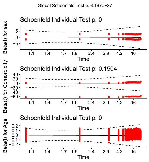
Figure 1.
The conventional Schoenfeld residuals from the application of the coronavirus disease 2019 (COVID-19) data set while taking the test p-value for the sex and comorbidity covariates into account.
Based on the above argument, in this research study, we proposed a more flexible parametric survival regression model called the extended-exponential-Weibull (ExEW) AFT model.
The main contribution of this study is to offer a useful addition to the toolkit for analyzing survival data that can be used with different hazard regression models in a more general way. There are several reasons why this work focuses on the extension of the AFT model under the ExEW HRF baseline. Firstly, although some classical distributions closed under the AFT model framework exist, none of them are versatile enough to include both monotone and non-monotone HRFs. Secondly, the parametric AFT model may produce more accurate estimates than the semi-parametric PH model. Thirdly, the use of the flexible distribution, which captures both monotone and non-monotone HRFs, is what makes our work distinctive and more appealing.
The motivations for the study can be briefly summarized as follows:
- To propose an ExEW-AFT model that is quite adaptable and can easily accommodate a variety of applications in reliability and survival analysis.
- The ExEW-AFT model could be viewed as a multiple-parameter survival regression, which is perhaps more adaptable than the common single-parameter survival regression model, including the Weibull and exponential AFT models.
- The results obtained with the application are considered the main contributions of this work.
- COVID-19 data from Sudan are used in the proposed model to determine how the disease risk factors affect the length of hospital stays.
The subsequent sections of the paper are structured as follows: The model formulation is presented in Section 2, and baseline HRFs are discussed in Section 3. The proposed model is examined in Section 4. Section 5 discusses the estimation of parameters. Section 6 presents the results of the simulation study. Application of the proposed model to COVID-19 data is offered in Section 7. Discussion is given in Section 8. In Section 9, some conclusions are cited.
2. AFT Model Formulation
For regression analysis of time-to-event data, there are two prevalent classes: odds-based and hazard-based regression models [2]. While the formulation in hazard-based models is dependent on the tractability of the baseline distribution’s HRF and cumulative HRF (CHRF), the formulation in odds-based models is dependent on the tractability of the odds function and its derivative [28].
The three common regression models in the context of hazard-based regression models are: PH [2], AFT [18], and accelerated hazard (AH) [20] models. On the other hand, the three most popular regression models in the context of odds-based regression models are proportional odds (PO) [29], accelerated odds (AO) [28], and AFT models. Hence, the AFT model is the only survival regression model that is closed under both odds-based and hazards-based regression models. The formulation of the AFT model is defined as follows:
Let be a vector of explanatory variables, and be the link function for the explanatory variables, where is a vector of regression coefficients. The HRF and survival function (SF) of the AFT model are expressed as follows:
and
The link function has the following properties:
- (i)
- for all
- (ii)
- is a one-to-one monotone function.
- (iii)
- .
In this study, we employed the link function as a standard exponential function. Hence, the HRF and SF of the AFT model can be re-written as follows:
and
3. The Baseline ExEW Distribution
In this study, we consider a very flexible lifetime distribution as the baseline distribution: the four-parameter ExEW distribution, also denoted as ExEW distribution, as presented in Mastor et al. [30] (with some corrections). Some background on it is given below. To begin, the cumulative distribution function (CDF) of the ExEW distribution takes the form
where , and are shape parameters, and is a scale parameter. The probability density function (PDF) corresponding to Equation (4) reduces to
The SF of the ExEW distribution is
The HRF of the ExEW distribution is expressed as
The corresponding CHRF is obtained as
By following the CDF in Equation (5), the HRF and CHRF for the baseline distribution have been corrected from the original equations in the original paper [30].
4. The Proposed Model
The proposed AFT model is developed by extending the ExEW distribution to incorporate covariates. The corresponding SF with covariate vector is given by
which corresponds to the SF of the ExEW distribution under the following configuration: and , that is
This demonstrates that, under the AFT model framework, the ExEW distribution is closed in the distributional sense.
Furthermore, the HRF with covariates is written as follows:
The PDF with covariates vector is given by
Single-parameter hazard-based regression (SPHBR) models are commonly used to relate covariates to one parameter of specific interest. In these SPHBR models, the role of the other (explanatory independent variables) parameters are often little more than to give the model sufficient generality to adapt to the data. A more tractable method is to relate these other parameters to covariates; this method is known as multi-parameter hazard-based regression (MPHBR) models [31,32,33,34]. The primary focus of this paper is the development of MPHBR models in the context of time-to-event analysis.
In our case, this is a multi-parameter AFT model, which is different from a single-parameter AFT model, like the Weibull AFT model or the log-logistic AFT model, among others, where only the scale parameter is changed. As a result, except for the parameter, the covariates influence the majority of the baseline distribution parameters. This is what makes our work unique and different from the common classical AFT models.
5. Estimation of the ExEW-AFT Parameters
To estimate the model parameters, maximum likelihood estimation (MLE) is used. Let be the lifetimes of n individuals. If the data are subject to right censoring, then , where corresponding to a potential censoring time for individual i. Suppose that for and otherwise. Hence, the observed data for an individual i consists of , for , where is a censoring time or lifetime according to whether 0 or 1, respectively and is a column vector of n external covariates for the ith individual.
In this scenario, non-informative censoring is assumed to be in place, meaning that neither the distribution of survival times nor the distribution of censoring times can be inferred from one another.
It is important to note that the assumption of non-informative censoring is justifiable when censoring is random (it is assumed that the failure rates for observations that are censored, uncensored, and remain in the risk set are equal) and/or independent (in other words, censorship is supposed to be random within any interested subgroup); for additional information on the non-informative censoring, see [35].
In this setting, the censored likelihood function is therefore defined as follows:
where is the vector of the involved parameters.
Based on Equation (13), the log-likelihood function for a parametric AFT model is defined as follows:
The Newton-Raphson optimization procedure can be used to directly optimize this, and interval estimates of the model parameters and hypothesis testing are both possible under the approximative normally distributed MLE estimates [8].
The likelihood function in the ExEW-AFT model is given by
where and of the ExEW-AFT model are derived from Equations (10) and (12), , . We recall that the censoring indicator satisfies if the observation is censored and if the observation is failed, and is the matrix of covariates, which is known as the design matrix or model matrix. After expressing the PDF in terms of HRF and SF and taking the logarithm of both sides of the likelihood function, the log-likelihood can be written as follows:
As a result, the full log-likelihood function for the ExEW-AFT model can be written as follows:
The MLE vector estimate of can be obtained by maximizing Equation (17) directly, with respect to the parameter vector . It is denoted by , so that , , , , and are the MLEs of a, b, c, and , respectively. By directly maximizing the total log-likelihood function with the aid of the tools R, MATHEMATICA, and MATLAB, the parameter estimations can be derived. R software is the program that is utilized in this work.
6. Simulation Study
In this section, we demonstrate the inferential capabilities of the proposed model using simulation results. Here, we demonstrate parameter estimation, the inclination to recover baseline HRF shapes using standard error (SE), average bias (AB), mean square error (MSE), and relative bias (RB) to pick models that accurately reflect the underlying HRF shape, and the effect of censoring proportions on the model’s inferential features.
6.1. Simulation Designs and Data Generation
Assuming the AFT regression model framework presented in Equation (11), we specifically simulated and 5000 data sets. Four variables were taken into account in the simulation study when we considered covariates. Two binary covariates, and , are produced using the Bernoulli (0.5) distribution, while two continuous covariates, and , were produced using the standard normal distribution. The covariate vector corresponds to the values for the AFT regression coefficients, which are selected to be . Using the inverse transform technique, the exponentiated Weibull (EW) distribution is used to simulate lifetime data from the AFT model framework [36].
In the regression equation, the effects of the covariates and the intercept are presumptive.
The PDF of the EW distribution takes the form
where are the distribution’s parameters.
6.2. Simulation Algorithm for the Proposed AFT Model
The following are the steps for executing the proposed AFT model:
- (i)
- Set the parameters of the model’s initial values,
- (ii)
- Utilize the inverse transform technique, create the lifetime data by inverting the CHRF of the proposed model,
- (iii)
- Utilize the various estimates to evaluate the estimations’ values,
- (iv)
- Analyze the inferential properties of the estimates, taking into account the SE, AB, MSE, and RB.
The Inverse Transform Technique
A popular probabilistic approach for creating datasets using regression survival models is the inverse transform technique [37,38,39,40]. This technique is based on the association between the CHRF of a lifetime random variable and a standard uniform random variable. Whenever the CHRF of the baseline distribution has an explicit form solution, it may be used, reversed, and easily used in R.
The CDF is derived from the SF as follows:
Given this, when generating data, if Y is a random variable that has this CDF, then follows a uniform distribution throughout the range and also follows a uniform distribution . At the end, for a realization u of U, by using the baseline CHRF , we get
The inverse of the CHRF must only be calculated if the baseline HRF is strictly positive for every t to simulate lifetime data. An expression of the random live corresponding to the AFT model is as follows:
In this study, we used the EW baseline distribution to generate survival times that can accommodate all of the basic HRF shapes, including decreasing, constant, increasing, unimodal, and bathtub shapes. The EW distribution is likewise closed in the context of the AFT regression model [18].
As a last comment, we recall that the CHRF of the EW model is
and thus the inverse of the CHRF is written as follows:
6.3. Simulated Scenarios
Based on the shapes in Figure 2, we provide the results of four simulation scenarios based on non-monotone HRF (bathtub or unimodal), and monotone HRF (decreasing or increasing) to evaluate the performance of the ExEW-AFT model in comparison with the Weibull AFT (W-AFT), log-logistic AFT (LL-AFT), and EW-AFT models and to investigate the impact of the baseline HRF shape specification on the AFT model’s inferential qualities.
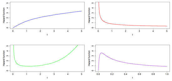
Figure 2.
HR shapes for generated distribution for all scenarios.
- Scenario 1: monotone (increasing) HRF:The lifetime data for this scenario are created using the EW model, and the parameter for ( and ). The censoring times are generated from the exponential distribution with rate parameter :For and .For and
- Scenario 2: monotone (decreasing) HRF:The EW model was used to create the lifetime data for this scenario, and the parameter values for (, and ). The censoring times are generated from the exponential distribution with rate parameter :For andFor and
- Scenario 3: non-monotone (bathtub) HRF:The EW model was used to create the lifetime data for this scenario, and the parameter values for ( and ). The censoring times are generated from the exponential distribution with rate parameter :For andFor and
- Scenario 4: non-monotone (unimodal) HRF:The EW model was used to create the lifetime data for this scenario, and the parameter values for ( and ). The censoring times are generated from the exponential distribution with rate parameter :For andFor and
Figure 2 shows the four Scenarios 1–4 (increasing (blue line), decreasing (red line), bathtub (green line), and unimodal (purple line) respectively), depending on the parameter values we chose, there were, on average, 20 and 30 percent censored observations.
6.4. Analyses of Simulated Data
To evaluate the inferential properties of the proposed models in all simulated scenarios, the ExEW-AFT model is fitted to the appropriate true generating model from the EW-AFT model. We also fitted the sub-models into each scenario. Furthermore, the estimates of the regression coefficients for each model are evaluated for stability based on the SE, RB, MSE, and the AB. These quantities are given by
and
where denotes each of the considered parameters.
Instead of examining the properties of the optimization process, our purpose was to examine the qualities of the estimates.
In all circumstances, we used the parameter values from the generating model as our optimization step starting points. The R programming language is used to do the analysis. With the aid of the R software “nlminb()”, the optimization stage is complete.
6.5. Performance Measures
The flexibility of the models for the covariates is evaluated in this study using measures such as the mean (estimated), AB, MSE, RB, and SE.
6.6. Simulation Results
According to the findings of scenario 1 in Table 1, Table 2, Table 3 and Table 4 the SE, AB, MSE, and RB indicate that the proposed model performed better than others. Furthermore, it appears that sample size and censoring percentage have an effect on how well models match data. When censoring and sample size are increased, our proposed ExEW-AFT model often outperforms the W-AFT and LL-AFT models. As anticipated, all models equally integrated the growing HRF. However, our proposed model performs better in the case of heavy censoring. Theoretically, the findings of scenario 2 in Table 5, Table 6, Table 7 and Table 8 show that all of the competing models can take into account the decreasing HRF shape. Our proposed ExEW-AFT model outperformed the W-AFT and LL-AFT models, and even the genuine produced model in terms of SE, AB, MSE, and RB. Moreover, when the censoring and sample size increase, our proposed model is once again the best-suited one and makes a wise choice of heavy censoring. The results of scenario 3 in Table 9, Table 10, Table 11 and Table 12 reveal that the only model that has the lowest value in terms of SE, AB, MSE, and RB is our proposed ExEW-AFT model. Generally, the W-AFT and LL-AFT models generated the least accurate estimates for AB, MSE, and RB according to Scenario 3, as expected (i.e., bathtub hazard). The findings of scenario 4 in Table 13, Table 14, Table 15 and Table 16 show that the proposed ExEW-AFT model produced estimates that had the lowest SE, AB, MSE, and RB values for all the regression coefficients while producing estimates that are equivalent to the genuine. Finally, the proposed AFT model outperforms the other competing models in all circumstances, including heavy censoring.

Table 1.
Simulation study for scenario 1 () with about 20% censored observations is used to compare model performance.
Table 2.
Simulation study for scenario 1 () with about 20% censored observations is used to compare model performance.
Table 3.
Simulation study for scenario 1 () with about 30% censored observations is used to compare model performance.
Table 4.
Simulation study for scenario 1 () with about 30% censored observations is used to compare model performance.
Table 5.
Simulation study for scenario 2 () with about 20% censored observations is used to compare model performance.
Table 6.
Simulation study for scenario 2 () with about 20% censored observations is used to compare model performance.
Table 7.
Simulation study for scenario 2 () with about 30% censored observations is used to compare model performance.
Table 8.
Simulation study for scenario 2 () with about 30% censored observations is used to compare model performance.
Table 9.
Simulation study for scenario 3 () with about 20% censored observations is used to compare model performance.
Table 10.
Simulation study for scenario 3 () with about 20% censored observations is used to compare model performance.
Table 11.
Simulation study for scenario 3 () with about 30% censored observations is used to compare model performance.
Table 12.
Simulation study for scenario 3 () with about 30% censored observations is used to compare model performance.
Table 13.
Simulation study for scenario 4 () with about 20% censored observations is used to compare model performance.
Table 14.
Simulation study for scenario 4 () with about 20% censored observations is used to compare model performance.
Table 15.
Simulation study for Scenario 4 () with about 30% censored observations is used to compare model performance.
Table 16.
Simulation study for scenario 4 () with about 30% censored observations is used to compare model performance.
7. Application to COVID-19 Data
In this Section, we demonstrate the adaptability and utility of the ExEW-AFT model, considering real-world right-censored COVID-19 data from Sudan.
7.1. Sudan COVID-19 Data
COVID-19 is an infectious illness. Many studies have been conducted since it was declared a global health emergency to better understand the disease’s clinical, epidemiological, and prognostic aspects [41,42,43,44,45].
In Sudan, the epidemiological data are disclosed by the epidemiology department of the federal ministry of health (FMH) www.fmoh.gov.sd (accessed on 25 May 2022). Therefore, according to the investigation of FMH, there are 35,321 patients who are infected with the virus. Moreover, every positive case between 13 March 2020 and 31 December 2021 is included in the study sample. The period from the date of admission until the date of the sample result is considered the length of the hospital stay.
Overview of Covariates of COVID-19 Data
For each patient (i = 1,…, 35,321), the following covariates are taken into account.
- y: The length of stay in the hospital (by days).
- Status: For censoring.
- : Age.
- : Sex group.
- : The comorbidity group.
Table 17 shows some descriptive statistics of these covariates. The average hospital stay lasts three days. The scaled total time on test (TTT) plot for the COVID-19 hazard rate shape is displayed in Figure 3, which shows that the hazard rate shape of COVID-19 is unimodal. The initial density shape of the length of stay in the hospital is reported using the non-parametric kernel density estimation (KDE) approach in Figure 4, beside the histogram. It is noted that the density is asymmetrical and positively skewed, which is a common feature for survival data and makes the normal distribution inappropriate to analyze [46]. This is one of the points that motivated us to use the ExEW distribution as a baseline hazard in the AFT model to fit this data. The box plot and violin plot in Figure 4 are used to identify the extremes, and they reveal that some of these extreme observations are recorded.
Table 17.
Statistical summary of the covariates for COVID-19 data.
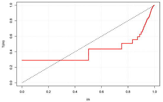
Figure 3.
TTT plot for the Sudan COVID-19 data.
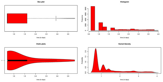
Figure 4.
Some non-parametric plots for the Sudan COVID-19 data.
Regarding the censoring status (0 is censored, 1 is observational lifetime), there is 7.3% censored in the sample of the study. Also, age as an explanatory variable refers to the patient’s age at diagnosis. Age is recorded as a continuous variable. Table 17 shows that the average age in the COVID-19 data set is 45 years, and the standard deviation is 6.226. Moreover, sex describes the gender of patients, which is a categorical variable with only two levels. Males are assigned the value 1, while females are assigned the value 2. There are 20,654 (58%) males and 14,667 (42%) females in the data.
It is recorded that COVID-19 is more common in men as compared to women in Sudan. Furthermore, the comorbidity status is a two-level categorical variable, with value 1 referring to a patient who has a chronic disease and value 2 referring to a patient who does not have a chronic disease. There are 845 (2.4%) patients who have a chronic disease in Sudan.
We analyze and compare the fitting of the ExEW-AFT model with that of sub-models such as the W-AFT, the exponentiated exponential (EE) AFT (EE-AFT), and the exponential Weibull AFT (ExW-AFT) models.
The AFT models for the competing models are as follows:
- The W-AFT model:
- The EE-AFT model:
- The ExW-AFT model:
The aforementioned Equations (27)–(29) demonstrate how the covariates act multiplicatively on time, causing an acceleration or a deceleration of time. The analytical measurements, such as the Bayesian information criterion (BIC), and the consistent Akaike information criterion (CAIC) were used to decide which AFT model matches the COVID-19 data the best. Additionally, goodness-of-fit metrics like the log-likelihood ratio test are used. The BIC is given by
and the CAIC is provided by
where ℓ refers to the log-likelihood function calculated at the MLEs, k for the number of model parameters, and n for the sample size.
7.2. Cox PH Model
To ascertain the relationship between survival time and the covariates thought to affect survival time, the Cox PH model is conducted. The Cox PH model parameters are estimated.
Table 18 shows the regression analysis of the Cox-PH model, including regression coefficients, SE, p-value, likelihood ratio test (LRT), and BIC values. Furthermore, all of the covariates (age, sex, and comorbidity) significantly affect the length of stay in the hospital at a 5% level of significance.
Table 18.
Results of Cox-PH model including the coefficients, SE, p-value, LRT, BIC, and CAIC.
Testing PH Assumption
The Schoenfeld residual is used in this study to test the PH assumption as follows: Based on the test, the Schoenfeld residuals are obtained for age and sex as covariates. The results in Table 19 provide evidence of the rejection of the assumption of PH for all covariates considered in the COVID-19 data. In other words, the PH models present an inadequate fit for this COVID-19 data.
Table 19.
Chi-square () test and p-value for Schoenfeld residual test at level of significance 1%.
7.3. AFT Model Analysis
In this subsection, we present the analysis of the ExEW-AFT, W-AFT, EE-AFT, and ExW-AFT models using the Sudan COVID-19 data.
We calculated the LRT statistics for the three sub-models. According to the LRT statistics in Table 20, the ExEW-AFT model fits the COVID-19 data the best. Table 21 showed that the SE of for the ExEW-AFT, W-AFT, EE-AFT, and ExW-AFT models is small enough. Moreover, at significance level, the parameters of all AFT models are significant, as shown in Table 22. Furthermore, the analytical measures of competing AFT models are shown in Table 23 which reveals that the ExEW-AFT model has the lowest BIC, and CAIC. In conclusion, the ExEW-AFT model is the best fit for the data among the W-AFT, EE-AFT, and ExW-AFT models under consideration. Moreover, at level of significance, all the covariates (age, sex, and comorbidity) significantly influence the length of stay at the hospital.
Table 20.
The LRT statistics for COVID-19 data at significance level 1%.
Table 21.
MLE fits of the ExEW, W, EW, and ExW AFT models with SE (in parentheses) for COVID-19 data.
Table 22.
z-value, p-value, and confidence interval (CI) for the AFT estimates for each model at the level of significance 5%.
Table 23.
The analytical performance measures for comparing AFT models for COVID-19 data.
Figure 5 shows the Kaplan–Meier (KM) survival curve, which indicates that the difference in survival times between the comorbidity group and the sexual group is statistically significant (p-value < 0.0001). Figure 6 depicts estimated HRFs for the competitive baseline hazards, and Figure 7 represents the average KM estimator and population SF. All of these figures show that our proposed ExEW-AFT model fits the data better than its competitors, including the Cox-PH and its sub-models.
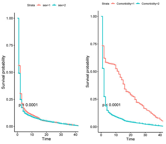
Figure 5.
The KM curves for time.
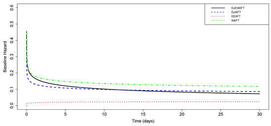
Figure 6.
Estimated HRFs for the competing baseline hazards.
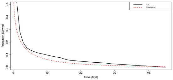
Figure 7.
Average KM estimator and population SF.
8. Discussion
The study was designed to produce a more versatile and general model than the Cox model. We assessed the performance of the proposed model’s estimators through a comprehensive Monte Carlo simulation study. The proposed model was also applied to Sudan COVID-19 Data. The choice of the AFT model is, therefore, sound as covariates directly relate to the time to event, which eases interpretability.
Considering the four different hazard rate (HR) shapes, including (increasing, decreasing, unimodal, and bathtub HR shapes), the simulation results showed that the ExEW model is capable of representing monotone decreasing, monotone increasing, unimodal, and bathtub HR functions more accurately than the existing AFT models such as: exponentiated-Weibull, Weibull, and log-logistic AFT models. Additionally, the SE, AB, RB, and MSE values showed that the proposed ExEW-AFT model performed well.
A real right-censored COVID-19 data set from Sudan reveals that it is misleading to trust the analysis based on the usual PH model, especially when the data exhibits characteristics such as the proportionality assumption [47]. This choice induces wrong conclusions, which, in turn, may lead to inappropriate clinical practices in terms of the best model that fits the data [11,48]. As demonstrated in our analysis, using different information criteria and some goodness-of-fit tests, including the likelihood ratio test, our proposed AFT model fits the data very well as compared to the common Cox-PH model and some other AFT single-parameter regression models (EW-AFT, W-AFT, and LL-AFT models). The three covariates (age, sex, and comorbidity) are significantly associated with the length of stay in the hospital. Previous studies have also shown the obtained results [49,50,51].
The developed model provided an important contribution to the toolset for assessing survival data and can be used with overall hazard regression models. However, our model has some limitations. The model is unable to handle survival data with crossing survival curves. Also, the future will see the development of residual analysis techniques and diagnostic measures for assessing the goodness of fit of the proposed model. Additionally, this work can be extended by proposing an AFT multi-parameter regression model for other types of censored survival data sets, including left censoring, interval censoring, middle censoring, and double censoring mechanisms. Furthermore, we can extend it to more complex survival models, including competing risk models, cure models, frailty models, and mixed effects AFT models, to apply to spatial and clustered survival data sets. In the analysis, only age, sex, and comorbidity covariates were used. Vaccination and place of residence (urban and rural) as variables to analyze the length of stay in the hospital could be very useful, but no information from those variables was collected.
9. Conclusions
In conclusion, the Ex-EW-AFT multi-parameter regression model’s flexibility could be highly helpful in representing many forms of time-to-event data that are difficult to predict accurately. Our model can be viewed as an attractive alternative for upcoming studies that assess censored lifetimes. As a result, the study includes a large number of simulation scenarios for evaluating the performance of our proposed model. The results demonstrated that the ExEW-AFT model performed effectively.
Future studies are advised to test the proposed model using other countries’ data sets as well as validate if the same factors would be important in a lifetime analysis. Finally, we recommend that in the future we look for a hazard-based regression model that can handle survival data with crossing survival curves.
Author Contributions
Conceptualization, A.B.S.M., A.S.A., O.N., J.M., C.C. and A.Z.A.; Data curation, O.N., J.M. and A.Z.A.; Formal analysis, A.B.S.M., A.S.A., O.N., J.M., C.C. and A.Z.A.; Methodology, A.B.S.M., A.S.A., O.N., J.M., C.C. and A.Z.A.; Investigation, A.B.S.M., A.S.A., O.N., J.M., C.C. and A.Z.A.; Software, A.B.S.M., O.N., J.M., C.C. and A.Z.A.; Project administration, A.S.A., O.N., J.M. and A.Z.A.; Supervision, O.N., J.M. and A.Z.A.; Writing—review and editing, A.B.S.M., A.S.A., O.N., J.M., C.C. and A.Z.A. All authors have read and agreed to the published version of the manuscript.
Funding
This research received no external funding.
Data Availability Statement
The corresponding author may be able to provide the real data that were used to illustrate the proposed approaches upon reasonable request. Due to ethical restrictions, the data are not publicly available.
Acknowledgments
The first author would like to thank the Pan African University, Institute for Basic Sciences, Technology, and Innovation (PAUSTI), Nairobi, Kenya. Additionally, We would like to thank the Federal Ministry of Health, Sudan for supporting this study with the required data.
Conflicts of Interest
The authors declare no conflict of interest.
References
- Cox, D.R. Regression models and life-tables. J. R. Stat. Soc. Ser. B 1972, 34, 187–202. [Google Scholar] [CrossRef]
- Khan, S.A.; Khosa, S.K. Generalized log-logistic proportional hazard model with applications in survival analysis. J. Stat. Distrib. Appl. 2016, 3, 1–18. [Google Scholar] [CrossRef]
- Rubio, F.J.; Remontet, L.; Jewell, N.P.; Belot, A. On a general structure for hazard-based regression models: An application to population-based cancer research. Stat. Methods Med. Res. 2019, 28, 2404–2417. [Google Scholar] [CrossRef] [PubMed]
- Ashraf-Ul-Alam, M.; Khan, A.A. Generalized Topp-Leone-Weibull AFT modelling: A Bayesian analysis with MCMC tools using R and stan. Austrian J. Stat. 2021, 50, 52–76. [Google Scholar] [CrossRef]
- Muse, A.H.; Mwalili, S.; Ngesa, O.; Alshanbari, H.M.; Khosa, S.K.; Hussam, E. Bayesian and frequentist approach for the generalized log-logistic accelerated failure time model with applications to larynx-cancer patients. Alex. Eng. J. 2022, 61, 7953–7978. [Google Scholar] [CrossRef]
- Withana Gamage, P.W.; McMahan, C.S.; Wang, L. A flexible parametric approach for analyzing arbitrarily censored data that are potentially subject to left truncation under the proportional hazards model. Lifetime Data Anal. 2022, 1–25. [Google Scholar] [CrossRef] [PubMed]
- Khan, S.A.; Basharat, N. Accelerated failure time models for recurrent event data analysis and joint modeling. Comput. Stat. 2022, 37, 1569–1597. [Google Scholar] [CrossRef]
- Lawless, J.F. Statistical Models and Methods for Lifetime Data; John Wiley & Sons: Hoboken, NJ, USA, 2011. [Google Scholar]
- Odell, P.M.; Anderson, K.M.; D’Agostino, R.B. Maximum likelihood estimation for interval-censored data using a Weibull-based accelerated failure time model. Biometrics 1992, 48, 951–959. [Google Scholar] [CrossRef] [PubMed]
- Huber, C.; Limnios, N.; Mesbah, M.; Nikulin, M.S. Mathematical Methods in Survival Analysis, Reliability and Quality of Life; John Wiley & Sons: Hoboken, NJ, USA, 2013. [Google Scholar]
- Aida, H.; Hayashi, K.; Takeuchi, A.; Sugiyama, D.; Okamura, T. An accelerated failure time cure model with shifted gamma frailty and its application to epidemiological research. Healthcare 2022, 10, 1383. [Google Scholar] [CrossRef]
- Kleinbaum, D.G.; Klein, M. Survival Analysis: A Self-Learning Text; Springer: New York, NY, USA, 2012; Volume 3. [Google Scholar]
- Collett, D. Modelling Survival Data in Medical Research; CRC Press: Boca Raton, FL, USA, 2015. [Google Scholar]
- Crowther, M.J.; Royston, P.; Clements, M. A flexible parametric accelerated failure time model and the extension to time-dependent acceleration factors. Biostatistics 2022. [Google Scholar] [CrossRef] [PubMed]
- Sinha, S.K. Robust estimation in accelerated failure time models. Lifetime Data Anal. 2019, 25, 52–78. [Google Scholar] [CrossRef]
- Zhang, Z.; Sinha, S.; Maiti, T.; Shipp, E. Bayesian variable selection in the accelerated failure time model with an application to the surveillance, epidemiology, and end results breast cancer data. Stat. Methods Med. Res. 2018, 27, 971–990. [Google Scholar] [CrossRef]
- Legrand, C. Advanced Survival Models; Chapman and Hall/CRC: Boca Raton, FL, USA, 2021. [Google Scholar]
- Khan, S.A. Exponentiated Weibull regression for time-to-event data. Lifetime Data Anal. 2018, 24, 328–354. [Google Scholar] [CrossRef]
- Santana, T.V.; Ortega, E.M.; Cordeiro, G.M. Generalized beta Weibull linear model: Estimation, diagnostic tools and residual analysis. J. Stat. Theory Pract. 2019, 13, 1–23. [Google Scholar] [CrossRef]
- Muse, A.H.; Ngesa, O.; Mwalili, S.; Alshanbari, H.M.; El-Bagoury, A.A.H. A flexible Bayesian parametric proportional hazard model: Simulation and applications to right-censored healthcare data. J. Healthc. Eng. 2022, 2022, 2051642. [Google Scholar] [CrossRef]
- Rinne, H. The Hazard Rate: Theory and Inference (with Supplementary MATLAB-Programs); Deutsche Nationalbibliothek: Leipzig, Germany, 2014. [Google Scholar]
- Ciampi, A.; Etezadi-Amoli, J. A general model for testing the proportional hazards and the accelerated failure time hypotheses in the analysis of censored survival data with covariates. Commun. Stat.-Theory Methods 1985, 14, 651–667. [Google Scholar] [CrossRef]
- Kalbfleisch, J.D.; Prentice, R.L. The Statistical Analysis of Failure Time Data; John Wiley & Sons: Hoboken, NJ, USA, 2011. [Google Scholar]
- Biazatti, E.C.; Cordeiro, G.M.; Rodrigues, G.M.; Ortega, E.M.; de Santana, L.H. A Weibull-beta prime distribution to model COVID-19 data with the presence of covariates and censored data. Stats 2022, 5, 1159–1173. [Google Scholar] [CrossRef]
- Cordeiro, G.M.; Rodrigues, G.M.; Ortega, E.M.; de Santana, L.H.; Vila, R. An extended Rayleigh model: Properties, regression and COVID-19 application. arXiv 2022, arXiv:2204.05214. [Google Scholar]
- Biazatti, E.C.; Cordeiro, G.M.; de Lima, M.d.C.S. The dual-Dagum family of distributions: Properties, regression and applications to COVID-19 data. Model Assist. Stat. Appl. 2022, 17, 199–210. [Google Scholar] [CrossRef]
- Rodrigues, G.M.; Ortega, E.M.; Cordeiro, G.M.; Vila, R. An extended Weibull regression for censored data: Application for COVID-19 in campinas, Brazil. Mathematics 2022, 10, 3644. [Google Scholar] [CrossRef]
- Muse, A.H.; Mwalili, S.; Ngesa, O.; Chesneau, C.; Alshanbari, H.M.; El-Bagoury, A.A.H. Amoud class for hazard-based and odds-based regression models: Application to oncology studies. Axioms 2022, 11, 606. [Google Scholar] [CrossRef]
- Economou, P.; Caroni, C. Parametric proportional odds frailty models. Commun. Stat. Comput. 2007, 36, 1295–1307. [Google Scholar] [CrossRef]
- Mastor, A.B.S.; Alfaer, N.M.; Ngesa, O.; Mung’atu, J.; Afify, A.Z. The extended exponential Weibull distribution: Properties, inference, and applications to real-life data. Complexity 2022, 2022, 4068842. [Google Scholar] [CrossRef]
- Jaouimaa, F.Z.; Ha, I.D.; Burke, K. Multi-parameter regression survival modelling with random effects. arXiv 2021, arXiv:2111.08573. [Google Scholar] [CrossRef]
- Peng, D.; MacKenzie, G.; Burke, K. A multiparameter regression model for interval-censored survival data. Stat. Med. 2020, 39, 1903–1918. [Google Scholar] [CrossRef] [PubMed]
- Burke, K.; Jones, M.; Noufaily, A. A flexible parametric modelling framework for survival analysis. J. R. Stat. Soc. Ser. C Appl. Stat. 2020, 69, 429–457. [Google Scholar] [CrossRef]
- Burke, K.; Eriksson, F.; Pipper, C. Semiparametric multiparameter regression survival modeling. Scand. J. Stat. 2020, 47, 555–571. [Google Scholar] [CrossRef]
- Kleinbaum, D.G.; Klein, M. Evaluating the proportional hazards assumption. In Survival Analysis; Springer: Berlin/Heidelberg, Germany, 2012; pp. 161–200. [Google Scholar]
- Leemis, L.M.; Shih, L.H.; Reynertson, K. Variate generation for accelerated life and proportional hazards models with time dependent covariates. Stat. Probab. Lett. 1990, 10, 335–339. [Google Scholar] [CrossRef]
- Leemis, L.M. Variate generation for accelerated life and proportional hazards models. Oper. Res. 1987, 35, 892–894. [Google Scholar] [CrossRef]
- Bender, R.; Augustin, T.; Blettner, M. Generating survival times to simulate Cox proportional hazards models. Stat. Med. 2005, 24, 1713–1723. [Google Scholar] [CrossRef]
- Austin, P.C. Generating survival times to simulate Cox proportional hazards models with time-varying covariates. Stat. Med. 2012, 31, 3946–3958. [Google Scholar] [CrossRef] [PubMed]
- Muse, A.H.; Mwalili, S.; Ngesa, O.; Chesneau, C.; Al-Bossly, A.; El-Morshedy, M. Bayesian and frequentist approaches for a tTractable parametric general class of hazard-based regression models: An application to oncology data. Mathematics 2022, 10, 3813. [Google Scholar] [CrossRef]
- Liu, H.; Tian, X. Data-driven optimal control of a SEIR model for COVID-19. arXiv 2020, arXiv:2012.00698. [Google Scholar] [CrossRef]
- Cordeiro, G.M.; Figueiredo, D.; Silva, L.; Ortega, E.M.; Prataviera, F. Explaining COVID-19 mortality rates in the first wave in Europe. Model Assist. Stat. Appl. 2021, 16, 211–221. [Google Scholar] [CrossRef]
- Marinho, P.R.D.; Cordeiro, G.M.; Coelho, H.F.; Brandão, S.C.S. Covid-19 in Brazil: A sad scenario. Cytokine Growth Factor Rev. 2021, 58, 51–54. [Google Scholar] [CrossRef] [PubMed]
- Cabore, J.W.; Karamagi, H.C.; Kipruto, H.K.; Mungatu, J.K.; Asamani, J.A.; Droti, B.; Titi-Ofei, R.; Seydi, A.B.W.; Kidane, S.N.; Balde, T.; et al. COVID-19 in the 47 countries of the WHO African region: A modelling analysis of past trends and future patterns. Lancet Glob. Health 2022, 10, e1099–e1114. [Google Scholar] [CrossRef]
- Kiarie, J.W.; Mwalili, S.M.; Mbogo, R.W. COVID-19 pandemic situation in Kenya: A data driven SEIR model. Med. Res. Arch. 2022, 10. [Google Scholar] [CrossRef]
- Alvares, D.; Lázaro, E.; Gómez-Rubio, V.; Armero, C. Bayesian survival analysis with BUGS. Stat. Med. 2021, 40, 2975–3020. [Google Scholar] [CrossRef]
- Patel, K.; Kay, R.; Rowell, L. Comparing proportional hazards and accelerated failure time models: An application in influenza. Pharm. Stat. J. Appl. Stat. Pharm. Ind. 2006, 5, 213–224. [Google Scholar] [CrossRef]
- Yang, J.; Zheng, Y.; Gou, X.; Pu, K.; Chen, Z.; Guo, Q.; Ji, R.; Wang, H.; Wang, Y.; Zhou, Y. Prevalence of comorbidities and its effects in patients infected with SARS-CoV-2: A systematic review and meta-analysis. Int. J. Infect. Dis. 2020, 94, 91–95. [Google Scholar] [CrossRef]
- Thiruvengadam, G.; Lakshmi, M.; Ramanujam, R. A study of factors affecting the length of hospital stay of COVID-19 patients by cox-proportional hazard model in a South Indian tertiary care hospital. J. Prim. Care Community Health 2021, 12, 21501327211000231. [Google Scholar] [CrossRef] [PubMed]
- Giacomelli, A.; Ridolfo, A.L.; Milazzo, L.; Oreni, L.; Bernacchia, D.; Siano, M.; Bonazzetti, C.; Covizzi, A.; Schiuma, M.; Passerini, M.; et al. 30-day mortality in patients hospitalized with COVID-19 during the first wave of the Italian epidemic: A prospective cohort study. Pharmacol. Res. 2020, 158, 104931. [Google Scholar] [CrossRef] [PubMed]
- Wu, S.; Xue, L.; Legido-Quigley, H.; Khan, M.; Wu, H.; Peng, X.; Li, X.; Li, P. Understanding factors influencing the length of hospital stay among non-severe COVID-19 patients: A retrospective cohort study in a Fangcang shelter hospital. PLoS ONE 2020, 15, e0240959. [Google Scholar] [CrossRef] [PubMed]
Disclaimer/Publisher’s Note: The statements, opinions and data contained in all publications are solely those of the individual author(s) and contributor(s) and not of MDPI and/or the editor(s). MDPI and/or the editor(s) disclaim responsibility for any injury to people or property resulting from any ideas, methods, instructions or products referred to in the content. |
© 2023 by the authors. Licensee MDPI, Basel, Switzerland. This article is an open access article distributed under the terms and conditions of the Creative Commons Attribution (CC BY) license (https://creativecommons.org/licenses/by/4.0/).