Abstract
A differential game with random duration is considered. The terminal time of the game is a random variable settled using a composite distribution function. Such a scenario occurs when the operating mode of the system changes over time at the appropriate switching points. On each interval between switchings, the distribution of the terminal time is characterized by its own distribution function. A method for solving such games using dynamic programming is proposed. An example of a non-renewable resource extraction model is given, where a solution of the problem of maximizing the total payoff in closed-loop strategies is found. An analytical view of the optimal control of each player and the optimal trajectory depending on the parameters of the described model is obtained.
Keywords:
differential game; random time horizon; composite distribution function; non-renewable resource extraction MSC:
37N40; 49N90; 91B76
1. Introduction
Differential games are widely used to model conflict-controlled processes that develop continuously in time. If the end time of the game is known, then the game is considered to be on a finite time interval. It is also common to consider games with an infinite horizon. However, when trying to describe real life processes, one often encounters uncertainty, in the sense that the terminal time of the game is not known in advance, but is the realization of some random variable. Such games are called games with random duration. For the first time, optimal control problems with uncertain lifetime were considered by Yaari in [1]. In this work, the use of such models was explained by the fact that the consumer, making plans for the future, one way or another, must take into account that he does not know how long he will live. Similar issues have been considered by Boukas in [2]. Later, this idea was widely applied in problems of dynamic games. The study of cooperative and non-cooperative differential games with random duration is presented by Shevkoplyas and Petrosyan in [3,4]. In work [5], for example, the randomness of the terminal time was explained by the life circle of technical equipments.
In some cases, the probability density function of the terminal time can change depending on different conditions and the standard distribution cannot fully simulate the random variable responsible for the moment of the end of the game. Such a scenario occurs when the operating mode of the system changes over time at the appropriate switching points and is characterized by its own distribution at each individual interval between switching. It can be used in financial models due to a possible financial credit crisis, as well as in modeling possible defaults and credit risks. Also in environmental models due to possible environmental disasters and climate change or in technical models due to equipment failures or different modes of technical equipment. In such problems, a composite distribution function for terminal time is used. By Zaremba et al. in [6], it is assumed that the duration of the game is a random variable corresponding to the discontinuous cumulative distribution function. Gromov and Gromova [7,8] considered games with random horizon and composite distribution function for terminal time as hybrid differential games, since payoffs of players in such games take the form of the sums of integrals with different, but adjoint time intervals. In [9], the differential game with composite distribution function for terminal time with two switching moments is investigated. Kamien and Schwartz [10] also used a composite distribution function in the model of the firm’s timing of a supramarginal technically modest innovation in a setting of rivalrous competition. Such function is used there to reflect the possibility that if one firm is first to introduce the product, rivals may alter their development rates. Other variants of models with switches at a random time moment can be found in [11]. In all these works, the solutions were found in the class of open-loop strategies using the maximum Pontryagin principle. However, since we are considering a process with many participants the players can deviate from some agreed course of action. In addition, only using the feedback strategies players can have a chance to react if they observe some deviations.
The purpose of this work is studying of games with a composite distribution function for terminal time in the class of feedback strategies using the dynamic programming methods [12]. The methods are illustrated on a class of optimal allocation models. As was mentioned in [13,14] such models found a lot of applications in economics in various forms: exhaustible resource extraction [15], cake-eating [16], and life-cycle saving [1]. The modern resource management has to take account of the possibility of regime shifts. In [17], for instance, a renewable resource model with the risk of regime shifts is considered. In such models, the state variable is the level of resources remaining. In addition, it is usually assumed that the utility functions of players are strictly concave and increasing. The relevance of the chosen model is confirmed, for example, by successful applying the resource extraction model to the coal mining problem in the form of a three-player differential cooperative game, where the players are the real companies with real life parameters in [18].
The paper is organized as follows. Section 2 gives the game formulation and the basic assumptions of the model. The following Section 3 presents a method for solving such games. The system of Hamilton–Jacobi–Bellman equations for the problem of maximizing the total payoff is given here. An illustrative example of a non-renewable resource extraction model is investigated in Section 4. The case of time-dependent switch is studied in Section 4.1. It is assumed that the switching moment of the composite distribution function is determined in advance. Section 4.2 demonstrates the state-dependent case, where switching time is not fixed, switching occurs when the system reaches a certain state.
2. Problem Statement
Consider differential n-player game presented by Gromov and Gromova in [7]. The game starts from initial state at the time and the terminal time T is the random variable, distributed on the time interval according to known composite distribution function with switches at fixed moments of time . Composite distribution function is defined as follows:
Here, is the set of distribution functions characterizing different modes of operation. are assumed to be absolutely continuous nondecreasing functions such that each distribution function converges to 1 asymptotically, i.e.,
To guarantee that composite distribution function is a continuous function suppose that , , Note that is defined as the left limit at , i.e., .
Further, we assume an existence of composite probability density function, that is defined as the derivative of distribution function, and has the following form:
For simplicity, we denote and
Let be an instantaneous payoff of the player i in the game at time t, , is the control of player i, are piecewise continuous functions. Assume that are differentiable, monotonically increasing and strictly concave.
The system dynamics is described by a first order differential equation:
where , (3) satisfy the standard requirements of existence and uniqueness. In particular, we assume that the function is continuously differentiable with regards to all its arguments. In addition, as usual for optimal allocation models, is decreasing on u.
The expected integral payoff of the player i is:
Note that no discount factor appears in the functional objectives of the problem, because the discount structure is built on the characteristics of the random terminal time.
In Section 2, the problem is formulated in general terms, but in Section 4, the functions take on a specific form. This model is chosen to simplify the solution, but the proposed method can, of course, be applied to a wider class of problems.
Assume that players cooperate in order to achieve the maximum total payoff. The optimization problem in this case can be written in the following form:
This problem was considered by Gromov and Gromova [7] in the class of open-loop strategies, where the control action selects according to the rule . Open-loop strategies are usually applied if the players cannot observe the state vector. Here we will restrict our attention to the case when the players apply feedback (or closed-loop) strategies, . This means that players observe the current value of the position . In general, such structure of strategies is useful in problems in which the players have a chance to react if they observe deviations from some agreed course of players’ action.
The expected payoff of the player in the subgame starting at the moment t from is evaluated by the formula:
The optimal cooperative strategies of players , are defined as follows:
The trajectory corresponding to the optimal cooperative strategies is the optimal cooperative trajectory .
3. System of Hamilton–Jacobi–Bellman Equations
We will solve the optimization problem using the Hamilton–Jacobi–Bellman equation.
Let – be the value of the Bellman function at :
Here – expected maximum total payoff of players in the subgame .
Consider subgame starting at the moment . We have a standard model of the game with random duration here, because there are no switches during the period . The expected gain in is as follows:
In [3], the Hamilton–Jacobi–Bellman equation for differential games with random duration was presented. Then according to the Bellman principle and [3] satisfies the equation:
at and the boundary condition One can note, that this boundary condition is quite often too strong as a sufficient optimality condition. Weaker conditions that apply to other classes of games can be found in [20,21].
Consider now the subgame at . The expected gain is as follows:
Then, taking in account the solution on the period , and according to [3], satisfies the equation:
at and the boundary condition
Increasing the range of t values step by step, we arrive at the Bellman function describing the maximum gain on .
So, for we have:
4. Example
Consider the game of non-renewable resource extraction by two players with instantaneous payoffs . Let . Suppose the players use identical equipment to operate the field and the probability of equipment failure is determined by the modes of operation. On this model starting at the time instant from the initial state , denotes the extraction effort of player i at time t. The system dynamics (the resource stock at time t available to the extraction) is described by the first order differential equation:
We have the following problem of optimal control:
4.1. Time-Dependent Switch
In this example, the duration of the game T is a random variable with composite distribution function defined by the rule (9):
Here, we assume that is a moment of switching of distribution function in this game. Let there be an ordered sequence of time moments . The optimal control problem can be decomposed into two problems, on the intervals , .
The distribution functions are defined using an exponential distribution:
Here, —parameters of exponential distributions, .
Let us find and :
Then, the composite distribution function for one switch at a fixed moment in time can be written in the form:
Figure 1 shows the example of such function.
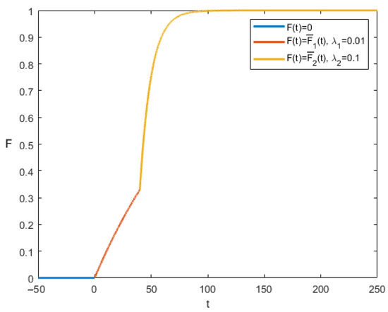
Figure 1.
Cumulative distribution function (, , ).
One reason for using a composite distribution function in such models could be that as a non-renewable resource is mined, the remaining resource may become increasingly difficult to extract. Which leads to another way of computing the probability of the end of the process. On the other hand the probability of a breakdown may depend on the development stage. It may be higher in the beginning of the process.
Consider a subgame , when . We need to solve the Hamilton–Jacobi–Bellman equation for this problem:
with the boundary condition
Here
The solution of (11) is found in the form
Substituting it into (11), we have the following differential equation for :
The solution of (12) is
The form of optimal control is as follows:
Denote . Now, solving the first order differential equation
with initial condition , we obtain:
According to the boundary condition , we obtain , then the solution on the interval takes the form:
Consider a subgame , when . Let be a Bellman function on this interval.
The Hamilton–Jacobi–Bellman equation for this problem with a random moment of game ending:
with the boundary condition
We will look for the Bellman function in the form . Then according to the boundary condition .
Note that
Substituting it into (13), we have the following differential equation for :
The solution of (14) is
The form of control is as follows:
Solving the first order differential equation
with initial condition , we obtain:
To sum up, the cooperative trajectory and optimal cooperative controls at intervals and have the form:
Finally, we show the graphical representation of the obtained solutions. We assume the following values of the parameters: , , , . Figure 2 shows the optimal control of player 1 (the blue line corresponds to , the red line for ). The optimal cooperative trajectory is presented by Figure 3.
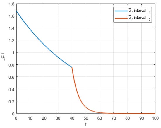
Figure 2.
Optimal control in the case of time-dependent switch.
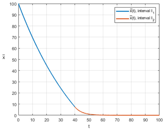
Figure 3.
Optimal cooperative trajectory in the case of time-dependent switch.
4.2. State-Dependent Switch
Let us assume now that the stock level of the resource can influence the probability of a regime shift, so the switching occurs not at some fixed point in time, but when a certain condition on the trajectory is satisfied. Within the framework of the model under consideration, such a condition may be the achievement of some predetermined level of resource stock.
Let the switching time is determined from the condition , where , is fixed.
On the interval the solution of Hamilton–Jacobi–Bellman Equation (11) is the same as in the previous case:
On the interval since is fixed we have a new condition on the trajectory that must be satisfied .
Here, the solution of (13) is found in the form
Substituting it into (13), we have the following differential equations for and :
with the boundary condition
The form of control is as follows:
Solving the first order differential equation
we obtain:
Taking into account the boundary conditions on the trajectory , , we obtain:
Finally, from (18) we have
Then, the maximum total payoff of players in the game has the following form:
The next problem is finding the optimal switching time :
Figure 4 demonstrates the graph of in our example if is a switching time and . This value means that when 80% of the initial stock of the resource is used up, a switch to another mode will occur. With the model parameters we have chosen (, ), it turns out that after switching, the probability of ending the game increases.
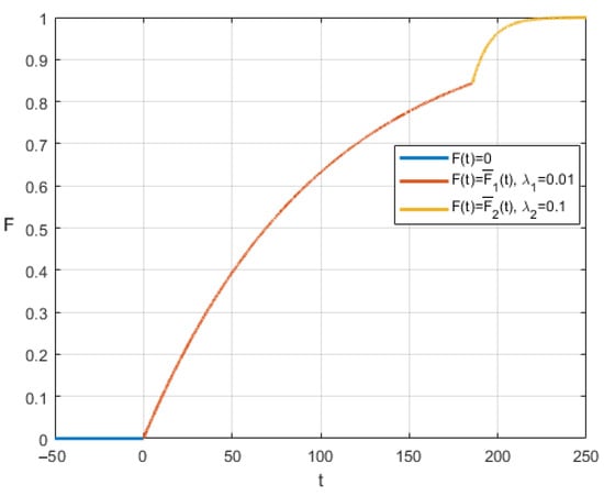
Figure 4.
Cumulative distribution function (, , , ).
To sum up, the cooperative trajectory and optimal cooperative controls at intervals and have the form:
Figure 5 and Figure 6 demonstrate graphs of optimal control and optimal cooperative trajectory for state-dependent case. Here, , , , .
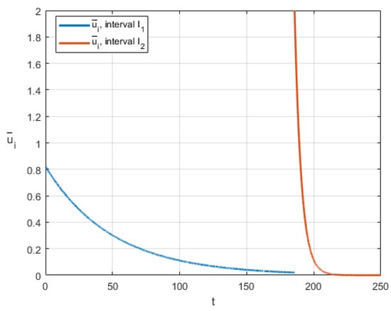
Figure 5.
Optimal control for state-dependent case.
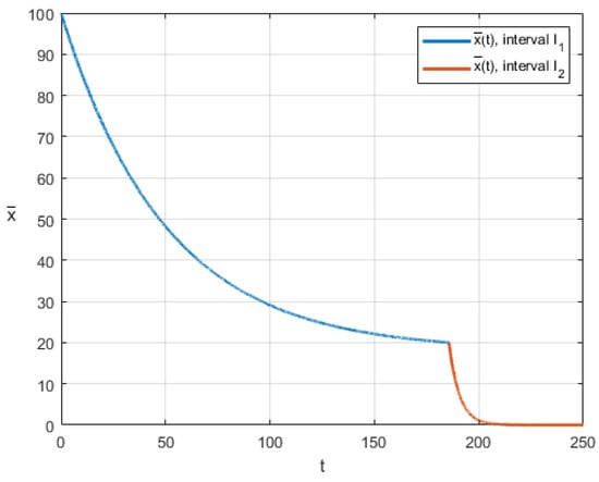
Figure 6.
Optimal cooperative trajectory for state-dependent case.
Note that in both cases, after switching the cumulative distribution function, players increase the intensity of resource extraction. This is because in our example , so the probability of ending the game increases in the second interval.
5. Conclusions
A method of the construction of optimal closed-loop cooperative strategies in differential games with random duration and composite distribution function of terminal time is proposed. Due to the switching modes of the distribution function, the payoffs of players in such games take the form of the sums of integrals with different, but adjoint time intervals. A method for solving such problems using dynamic programming is explored. It is shown that finding the optimal control in such problems is reduced to the sequential consideration of intervals, starting from the last switching, and compiling the Hamilton–Jacobi–Bellman equation on each interval, and boundary solutions are obtained from the solution on the interval considered earlier. An example of a non-renewable resource extraction model is studied. Two cases are considered. In the first one, the switching of the terminal time distribution function occurs at a predetermined time. In the second, the switching depends on the state of the system. An analytical view of the optimal control and the optimal cooperative trajectory is obtained. It was demonstrated how the optimal controls of the players changes when switching the distribution function.
The future research will consist in studying the non-cooperative case of the game and time-consistency problem for obtained solutions.
Author Contributions
Conceptualization, A.T.; methodology, T.B. and A.T.; formal analysis, T.B. and A.T.; investigation, T.B. and A.T.; writing—original draft preparation, T.B.; writing—review and editing, T.B. and A.T.; visualization, A.T.; funding acquisition, A.T. All authors have read and agreed to the published version of the manuscript.
Funding
This research was funded by RFBR and DFG, project number 21-51-12007.
Institutional Review Board Statement
Not applicable.
Informed Consent Statement
Not applicable.
Data Availability Statement
Not applicable.
Conflicts of Interest
The authors declare no conflict of interest.
References
- Yaari, M.E. Uncertain Lifetime, Life Insurance, and the Theory of the Consumer. Rev. Econ. Stud. 1965, 32, 137–150. [Google Scholar] [CrossRef]
- Boukas, E.K.; Haurie, A.; Michel, P. An Optimal Control Problem with a Random Stopping Time. J. Optim. Appl. 1990, 64, 471–480. [Google Scholar] [CrossRef]
- Shevkoplyas, E.V. The Hamilton–Jacobi–Bellman equation for a class of differential games with random duration. Math. Game Theory Appl. 2009, 1, 98–118, Erratum in Autom. Remote Control. 2014, 75, 959–970. [Google Scholar] [CrossRef]
- Petrosyan, L.A.; Shevkoplyas, E.V. Cooperative Solution for Games with Random Duration. Game Theory Appl. 2003, 9, 125–139. [Google Scholar]
- Shevkoplyas, E.; Sergey Kostyunin, S. Modeling of Environmental Projects under Condition of a Random Time Horizon. Contrib. Game Theory Manag. 2011, 4, 447–459. [Google Scholar]
- Zaremba, A.; Gromova, E.; Tur, A. A Differential Game with Random Time Horizon and Discontinuous Distribution. Mathematics 2020, 8, 2185. [Google Scholar] [CrossRef]
- Gromov, D.; Gromova, E. Differential games with random duration: A hybrid systems formulation. Contrib. Game Theory Manag. 2014, 7, 104–119. [Google Scholar]
- Gromov, D.; Gromova, E. On a Class of Hybrid Differential Games. Dyn. Games Appl. 2017, 7, 266–288. [Google Scholar] [CrossRef]
- Balas, T.N. One hybrid optimal control problem with multiple switches. Control Process. Stab. 2022, 9, 379–386. [Google Scholar]
- Kamien, M.I.; Schwartz, N.L. Timing of innovations under rivalry. Econometrica 1972, 40, 43–60. [Google Scholar] [CrossRef]
- Zaremba, A.P. Cooperative differential games with the utility function switched at a random time moment. Math. Game Theory Appl. 2022, 14, 31–50, Erratum in Autom. Remote. Vol. 2022, 83, 1652–1664. [Google Scholar] [CrossRef]
- Bellman, R. Dynamic Programming; Princeton University Press: Princeton, NJ, USA, 1957. [Google Scholar]
- Leung, S.F. Cake eating, exhaustible resource extraction, life-cycle saving, and non-atomic games: Existence theorems for a class of optimal allocation problems. J. Econ. Dyn. Control 2009, 33, 1345–1360. [Google Scholar] [CrossRef]
- Clemhout, S.; Wan, H.Y. On games of cake-eating. In Dynamic Policy Games in Economics; van der Ploeg, F., de Zeeuw, A., Eds.; North Holland: New York, NY, USA, 1989. [Google Scholar]
- Hotelling, H. The Economics of Exhaustible Resources. In Classic Papers in Natural Resource Economics; Gopalakrishnan, C., Ed.; Palgrave Macmillan: London, UK, 1954. [Google Scholar]
- Gale, D. On Optimal Development in a Multi-Sector Model. Rev. Econ. Stud. 1967, 34, 1–18. [Google Scholar] [CrossRef]
- De Zeeuw, A.; He, X. Managing a renewable resource facing the risk of a regime shift in the ecological system. Resour. Energy Econ. 2017, 48, 42–54. [Google Scholar] [CrossRef]
- Gromova, E.; Bolatbek, A. Value of Information in the Deterministic Optimal Resource Extraction Problem with Terminal Constraints. Appl. Sci. 2023, 13, 703. [Google Scholar] [CrossRef]
- Kostyunin, S.; Shevkoplyas, E. On simplification of integral payoff in the differential games with random duration. Vestn. St. Petersburg Univ. Math. 2011, 4, 47–56. [Google Scholar]
- Wiszniewska-Matyszkiel, A. On the terminal condition for the Bellman equation for dynamic optimization with an infinite horizon. Appl. Math. Lett. 2011, 24, 943–949. [Google Scholar] [CrossRef]
- Dockner, E.J.; Jorgensen, S.; van Long, N.; Sorger, G. Differential Games in Economics and Management Science; Cambridge University Press: Cambridge, UK, 2000. [Google Scholar]


Disclaimer/Publisher’s Note: The statements, opinions and data contained in all publications are solely those of the individual author(s) and contributor(s) and not of MDPI and/or the editor(s). MDPI and/or the editor(s) disclaim responsibility for any injury to people or property resulting from any ideas, methods, instructions or products referred to in the content. |
© 2023 by the authors. Licensee MDPI, Basel, Switzerland. This article is an open access article distributed under the terms and conditions of the Creative Commons Attribution (CC BY) license (https://creativecommons.org/licenses/by/4.0/).