Codimension-Two Bifurcations of a Simplified Discrete-Time SIR Model with Nonlinear Incidence and Recovery Rates

Abstract

In this paper, a simplified discrete-time SIR model with nonlinear incidence and recovery rates is discussed. Here, using the integral step size and the intervention level as control parameters, we mainly discuss three types of codimension-two bifurcations (fold-flip bifurcation, 1:3 resonance, and 1:4 resonance) of the simplified discrete-time SIR model in detail by bifurcation theory and numerical continuation techniques. Parameter conditions for the occurrence of codimension-two bifurcations are obtained by constructing the corresponding approximate normal form with translation and transformation of several parameters and variables. To further confirm the accuracy of our theoretical analysis, numerical simulations such as phase portraits, bifurcation diagrams, and maximum Lyapunov exponents diagrams are provided. In particular, the coexistence of bistability states is observed by giving local attraction basins diagrams of different fixed points under different integral step sizes. It is possible to more clearly illustrate the model’s complex dynamic behavior by combining theoretical analysis and numerical simulation.

1. Introduction

Throughout time, human beings have been plagued by various epidemic diseases, such as plague [1], cholera [2], influenza [3], etc. In the process of human struggle against epidemic diseases, medical personnel have developed vaccines against various viruses and proposed many epidemic prevention measures. In addition, mathematicians have also made important contributions in curbing the spread of diseases. The time from the outbreak of the epidemic disease to its control, the number of people in contact with the disease who need to be quarantined, and the number of infected people at a certain time during the development of the epidemic disease can be more or less determined from the perspective of mathematical models. In 1927, Kermack and Mckendrick analyzed the number of patients with plague and the survival days of patients and finally put forward a landmark model in mathematical epidemiology: the SIR model [4]. Up to now, the vast majority of studies analyzing infectious diseases from a mathematical perspective have worked in the shadow of this model. In 2005, Zhang et al. proposed a compartmental model that modeled the SARS control strategies implemented by the Chinese government after the middle of April 2003 [5]. In 2011, Yang et al. used methods such as grey prediction and cellular automata to study the mathematical model of H1N1 influenza [6]. In the research and prediction of the COVID-19 epidemic, many scholars used the infectious disease dynamics model as a basic research tool and proposed various improvement methods to enrich the classical infectious disease dynamics model, enabling it to more objectively describe the actual situation of epidemic transmission and making more reasonable predictions about the development trend of the epidemic. Many effective suggestions have been provided for prevention, control, and governance [7,8,9].

In recent years, research on dynamical systems has undergone qualitative changes. Dynamical systems are an interdisciplinary field that can be applied not only to the study of epidemic diseases, but also to many other fields, such as predator–prey models [10] and tumor models [11]. For the research of epidemic diseases, we generally apply mathematical models to characterize their rich dynamic behavior [12]. Some mathematical models are designed to target specific diseases [13], but most are suitable for general studies of the laws of various epidemic diseases. Most models of epidemic disease are ordinary differential equations. However, compared to continuous models, discrete-time dynamic models are considerably more straightforward and computationally efficient. Most discrete-time epidemic models not only are simple analogies of continuous epidemic models, but also show complex dynamic behaviors that the corresponding continuous models cannot show. The discrete-time model is capable of producing extremely complicated dynamics, even in a one-dimensional instance [14]. Many interesting and important research works can be found in [15,16,17,18,19] and the references cited therein.

As we all know, bifurcation theory is a vital tool for understanding the behavioral characteristics of dynamic systems. In applied mathematics research, period-doubling bifurcation and Neimark–Sacker bifurcation are two important phenomena of the discrete-time dynamical model [19,20,21]. The period-doubling bifurcation process is a typical path to chaos, which can be considered as a way to enter chaos from the periodic window. Neimark–Sacker bifurcation is a classic tool for studying the generation and death of small-amplitude periodic solutions of discrete dynamic systems. Liu et al. discretized a discrete-time gene regulatory network system by using the forward Euler’s method. Theoretical analysis and numerical simulations illustrate some interesting dynamical behaviors such as period-doubling bifurcation, Neimark–Sacker bifurcation, and chaos [22]. Discrete-time dynamical models, however, frequently incorporate a large number of parameters, and the models are unavoidably affected by two or more parameters. Therefore, it is of more practical significance to study the complex behaviors of a nonlinear model on a two-dimensional parameter plane or even a higher-dimensional parameter space. Eskandari and Alidousti reported that an SIR model undergoes codimension-two bifurcations with 1:2 resonance, 1:3 resonance, and 1:4 resonance. The rich dynamics of the model on the two-parameter plane for the first iteration were discussed [23]. Li et al. studied multiple and generic bifurcations of a discrete Hindmarsh–Rose model. Different kinds of critical cases of codimension-one and -two bifurcations are computed by the inner product method. The richer and more complex behaviors under higher iterations and the bifurcation distributions of codimension-two bifurcation points are investigated [24]. In addition, various types of codimension-one and -two bifurcations have been investigated in [25,26,27,28,29,30,31,32,33] and the references cited therein.

For local bifurcations of nonhyperbolic fixed points, universal bifurcation diagrams are given by the topological normal form method. Bifurcation diagrams are not entirely chaotic, and different strata of bifurcation diagrams in generic systems interact by following specific rules. This makes the bifurcation diagrams of systems arising in many different applications look similar. To this end, a system should be transformed into its topological normal forms whose highest order is the second or third order by smooth reversible changes of the coordinate and the parameter. The topological equivalent systems that have qualitatively similar or equivalent bifurcation diagrams to the original system can be obtained after these transformations [34].

However, there are still many difficulties in studying codimension-two bifurcations due to the influence of higher-order nonlinear terms. The complex dynamics of even elementary dynamical systems cannot be clearly demonstrated by theoretical analysis. Some researchers have explored the use of computers to model the dynamics within the local parameter variation. Therefore, the numerical methods are helpful not only to validate our analytical results but also to better demonstrate and understand the dynamics of the model [14]. In this paper, we analyze a discrete-time model with the help of various numerical tools and techniques. For example, MatcontM is a bifurcation continuation package for discrete-time dynamical systems [35,36,37,38].

Alshmmari and Khan [39] proposed an SIR model with nonlinear incidence and nonlinear recovery rates consisting of three nonlinear differential equations as

$$\left\{\begin{array}{c}\frac{\mathrm{d}S}{\mathrm{d}t}=A-\frac{\beta IS}{k+I}-\mu S,\hfill \\ \frac{\mathrm{d}I}{\mathrm{d}t}=\frac{\beta IS}{k+I}-\left({\alpha }_0+\left({\alpha }_1-{\alpha }_0\right)\frac{b}{b+I}\right)I-\left(\gamma +\mu \right)I,\hfill \\ \frac{\mathrm{d}R}{\mathrm{d}t}=\left({\alpha }_0+({\alpha }_1-{\alpha }_0)\frac{b}{b+I}\right)I-\mu R,\hfill \end{array}\right.$$

(1)

where $S\left(t\right)$, $I\left(t\right)$, and $R\left(t\right)$ denote the numbers of susceptible, infected, and recovered individuals at time t, respectively. $A,\gamma$, and $\mu$ represent the birth rate, the death rate due to disease, and the natural death rate of each species, respectively. $\frac{\beta IS}{k+I}$ and ${\alpha }_0+\left({\alpha }_1-{\alpha }_0\right)\frac{b}{b+I}$ represent the nonlinear incidence rate and nonlinear recovery rate, respectively. ${\alpha }_1$ and ${\alpha }_0$ ($0<{\alpha }_0<{\alpha }_1$ ) denote the maximum and minimum per capita recovery rates, respectively. b indicates the impact of the number of hospital beds on the transmission of infectious diseases. k represents the intervention levels and determines the shape of the incidence rate.

Since $R\left(t\right)$ does not appear in the first two equations of model (1), it is sufficient only to consider the following reduced model, which consists of the first two equations

$$\left\{\begin{array}{c}\frac{\mathrm{d}S}{\mathrm{d}t}=A-\frac{\beta IS}{k+I}-\mu S,\hfill \\ \frac{\mathrm{d}I}{\mathrm{d}t}=\frac{\beta IS}{k+I}-\left({\alpha }_0+\left({\alpha }_1-{\alpha }_0\right)\frac{b}{b+I}\right)I-\left(\gamma +\mu \right)I,\hfill \end{array}\right.$$

(2)

where $R\left(t\right)=N\left(t\right)-S\left(t\right)-I\left(t\right)$, and $N\left(t\right)$ is the total population.

Here, we discuss the complex dynamics of a discrete-time version SIR model, which is obtained from the simplified model (2) by adopting the forward Euler’s method and replacing $S\to x$ and $I\to y$ as follows:

$$\left(\begin{array}{c}x\\ y\end{array}\right)\mapsto \mathcal{N}(x,y,\vartheta )=\left(\begin{array}{c}x+h\left(A-\frac{\beta yx}{k+y}-\mu x\right)\\ y+h\left(\frac{\beta yx}{k+y}-\left({\alpha }_0+\left({\alpha }_1-{\alpha }_0\right)\frac{b}{b+y}\right)y-\left(\gamma +\mu \right)y\right)\end{array}\right),$$

(3)

where $A,\beta ,{\alpha }_0,{\alpha }_1,\mu ,\gamma ,b$, and $k$ are defined in model (1), h is the integral step size for discretization, and $\vartheta =(h,A,\beta ,{\alpha }_0,{\alpha }_1,\mu ,\gamma ,b,k)$. In fact, we have discussed some dynamics of model (3) in [40], such as the stability of fixed points, some codimension-one bifurcations (transcritical, period-doubling, and Neimark–Sacker bifurcations) and a codimension-two bifurcation (1:2 resonance) of non-hyperbolic fixed points. In [40], through numerical continuation by using MatcontM, we found that besides the above bifurcations, the model also has other codimension-two bifurcation phenomena, such as fold-flip bifurcation, 1:3 resonance, and 1:4 resonance. However, there is no rigorous theoretical support for these codimension-two bifurcations but only numerical continuation results in our previous work. In this paper, we give a detailed theoretical analysis of these interesting codimension-two bifurcations of model (3) by constructing an approximate normal form when k and h are used as the bifurcation parameters. Some new numerical simulations of codimension-two bifurcations are also given to show that there are abundant and complex dynamical behaviors in model (3) with the change of parameters k and h by using Matlab and the standard numerical software package MatcontM (the version is Matcontm5p4). In particular, we observe the local dynamics, such as local attraction basins in the neighborhood of fixed points.

The outline of this paper is as follows. Firstly, the existence and stability of the fixed points of model (3) are given in Section 2. Secondly, theoretical analysis of the codimension-two bifurcations (fold-flip bifurcation, 1:3 resonance, and 1:4 resonance) of model (3) is discussed in Section 3. Some numerical continuation and numerical simulation results for illustrating the theoretical analysis are provided in Section 4. In particular, local attraction basin diagrams are given to demonstrate the rich dynamics in the neighborhood of the codimension-two bifurcation points. Finally, this paper ends with a brief conclusion in Section 5.

2. Existence and Stability of Fixed Points

In this section, the parameter conditions for the existence and stability of fixed points in the discrete-time model (3) are given. The detailed derivations are given in [40]. For convenience sake and quick reference, we summarize them as follows.

2.1. Existence of Fixed Points

The study of the bifurcation structures of a model usually starts from the analysis of fixed points. The fixed points of model (3) are positive solutions to

$$\left\{\begin{array}{c}A-\frac{\beta yx}{k+y}-\mu x=0,\hfill \\ \frac{\beta yx}{k+y}-\left({\alpha }_0+\left({\alpha }_1-{\alpha }_0\right)\frac{b}{b+y}\right)y-\left(\gamma +\mu \right)y=0.\hfill \end{array}\right.$$

(4)

There are at most two kinds of fixed points in model (3). One is the disease-free fixed point $E_0\left(\frac{A}{\mu },0\right)$, and the other is the endemic fixed points $E_i(x_i^{\ast },y_i^{\ast })(i=1,2)$, if and only if $y_i^{\ast }$$(i=1,2)$ is a positive root of the following quadratic equation:

$$f\left(y\right):=C_1{y}^2+C_{2}y+C_3,$$

(5)

where

$$\begin{array}{c}\hfill C_1=(\beta +\mu )({\alpha }_0+\gamma +\mu ),C_2=k\mu ({\alpha }_0+\gamma +\mu )+b(\beta +\mu )({\alpha }_1+\gamma +\mu )-\beta A,C_3=b\left(k\mu ({\alpha }_1+\gamma +\mu )-A\beta \right).\end{array}$$

(6)

Furthermore,

$$x_i^{\ast }=\frac{A(k+y_i^{\ast })}{(\beta +\mu )y_i^{\ast }+k\mu }(i=1,2).$$

The solutions of Equation (5) are computed by

$$y_i^{\ast }=\frac{-C_2\pm \sqrt{\Delta }}{2C_1}(i=1,2),$$

where

$$\begin{array}{cc}\hfill \Delta =& C_2^2-4C_1{C}_3\hfill \\ \hfill =& {\left(k\mu ({\alpha }_0+\gamma +\mu )+b(\beta +\mu )({\alpha }_1+\gamma +\mu )-\beta A\right)}^2\hfill \\ \hfill & -4b(\beta +\mu )({\alpha }_0+\gamma +\mu )\left(k\mu ({\alpha }_1+\gamma +\mu )-A\beta \right).\hfill \end{array}$$

(7)

When $\Delta =0$, the two fixed points $E_1$ and $E_2$ collide and merge into $E(x,y)$, where

$$\left\{\begin{array}{c}x=\frac{\left(Ak(2\beta +3\mu )+b(\beta +\mu )\right)({\alpha }_1+\gamma +\mu )-Ak(2\beta +3\mu )({\alpha }_1-{\alpha }_0)-A^2\beta }{\left(b(\beta +\mu )+3k\mu \right)({\alpha }_1+\gamma +\mu )-3k\mu ({\alpha }_1-{\alpha }_0)-A\beta (\beta +\mu )},\hfill \\ y=\frac{\beta A-k\mu ({\alpha }_0+\gamma +\mu )-b(\beta +\mu )({\alpha }_1+\gamma +\mu )}{2(\beta +\mu )({\alpha }_0+\gamma +\mu )}.\hfill \end{array}\right.$$

As we can see from (6), $C_1>0$ when the parameters are all positive, $C_2>0$ when $b>\frac{A\beta -k\mu ({\alpha }_0+\gamma +\mu )}{(\beta +\mu )({\alpha }_1+\mu +\gamma )}$, and $C_3>0$ when $k>\frac{\beta A}{\mu ({\alpha }_1+\gamma +\mu )}$. We obtain the following results.

Lemma 1.

The fixed points of model (3) are as follows: model (3) always has a disease-free fixed point $E_0\left(\frac{A}{\mu },0\right)$ for all positive parameters. And for the endemic fixed point(s), we have:

(I) 

$C_1>0$ and $C_3<0$, model (3) has only one endemic fixed point $E_2$.

(II) 

$C_1>0$ and $C_3=0$,

(i) 

When $C_2<0$, model (3) has only one endemic fixed point $E_2$.

(ii) 

When $C_2⩾0$, model (3) has no endemic fixed points.

(III) 

$C_1>0$ and $C_3>0$,

(i) 

When $C_2<0$, there are two endemic fixed points $E_1,E_2$ if $\Delta >0$, one endemic fixed point E if $\Delta =0$, and no endemic fixed point if $\Delta <0$.

(ii) 

When $C_2⩾0$, model (3) has no endemic fixed points.

The parameter conditions for the existence of fixed points are summarized in Table 1.

Table 1. Existence of fixed points.

Conditions			Fixed Points
All the parameters are positive			$E_0$
$k<\frac{\beta A}{\mu ({\alpha }_1+\gamma +\mu )}$	$b>0$		$E_0,E_2$
$k=\frac{\beta A}{\mu ({\alpha }_1+\gamma +\mu )}$	$0<b<\frac{A\beta -k\mu ({\alpha }_0+\gamma +\mu )}{(\beta +\mu )({\alpha }_1+\mu +\gamma )}$		$E_0,E_2$
	$b⩾\frac{A\beta -k\mu ({\alpha }_0+\gamma +\mu )}{(\beta +\mu )({\alpha }_1+\mu +\gamma )}$		$E_0$
$k>\frac{\beta A}{\mu ({\alpha }_1+\gamma +\mu )}$	$0<b<\frac{A\beta -k\mu ({\alpha }_0+\gamma +\mu )}{(\beta +\mu )({\alpha }_1+\mu +\gamma )}$	$\Delta <0$	$E_0$
		$\Delta =0$	$E_0,E$
		$\Delta >0$	$E_0,E_1,E_2$
	$b⩾\frac{A\beta -k\mu ({\alpha }_0+\gamma +\mu )}{(\beta +\mu )({\alpha }_1+\mu +\gamma )}$		$E_0$

2.2. Stability of Fixed Points

2.2.1. Stability of the Disease-Free Point $E_0\left(\frac{A}{\mu },0\right)$

When all the parameters are positive, there is always the disease-free point $E_0\left(\frac{A}{\mu },0\right)$, whose properties are given in Table 2.

Table 2. Stability of the disease-free fixed point $E_0$.

Conditions		Eigenvalues		Properties
		${\mathit{\lambda }}_{\mathbf{1}}=\mathbf{1}-\mathit{h}\mathit{\mu }$	${\mathit{\lambda }}_{\mathbf{2}}=\mathbf{1}+\mathit{h}(\frac{\mathit{\beta }\mathit{A}}{\mathit{\mu }\mathit{k}}-{\mathit{\alpha }}_{\mathbf{1}}-\mathit{\gamma }-\mathit{\mu })$
$0<h<\frac{2}{\mu }$	$\frac{\beta A}{\mu ({\alpha }_1+\gamma +\mu )}<k<\frac{\beta A}{\mu ({\alpha }_1+\gamma +\mu -\frac{2}{h})}$, $h>\frac{2}{{\alpha }_1+\gamma +\mu }$	$|{\lambda }_1|<1$	$|{\lambda }_2|<1$	Stable
	$k=\frac{\beta A}{\mu ({\alpha }_1+\gamma +\mu -\frac{2}{h})},h>\frac{2}{{\alpha }_1+\gamma +\mu }$		$|{\lambda }_2|=1$	Non-hyperbolic
	$k=\frac{\beta A}{\mu ({\alpha }_1+\gamma +\mu )}$
	$k>\frac{\beta A}{\mu ({\alpha }_1+\gamma +\mu -\frac{2}{h})},h>\frac{2}{{\alpha }_1+\gamma +\mu }$ or $k<\frac{\beta A}{\mu ({\alpha }_1+\gamma +\mu )}$		$|{\lambda }_2|>1$	Unstable
$h=\frac{2}{\mu }$	$\frac{\beta A}{\mu ({\alpha }_1+\gamma +\mu )}<k<\frac{\beta A}{\mu ({\alpha }_1+\gamma )}$	$|{\lambda }_1|=1$	$|{\lambda }_2|<1$	Non-hyperbolic
	$k=\frac{\beta A}{\mu ({\alpha }_1+\gamma )}$		$|{\lambda }_2|=1$
	$k=\frac{\beta A}{\mu ({\alpha }_1+\gamma +\mu )}$
	$k>\frac{\beta A}{\mu ({\alpha }_1+\gamma )}$ or $k<\frac{\beta A}{\mu ({\alpha }_1+\gamma +\mu )}$		$|{\lambda }_2|>1$	Unstable
$h>\frac{2}{\mu }$	$k<\frac{\beta A}{\mu ({\alpha }_1+\gamma +\mu -\frac{2}{h})}$ or $k>\frac{\beta A}{\mu ({\alpha }_1+\gamma +\mu )}$	$|{\lambda }_1|>1$	$|{\lambda }_2|<1$
	$k=\frac{\beta A}{\mu ({\alpha }_1+\gamma +\mu -\frac{2}{h})}$		$|{\lambda }_2|=1$
	$k=\frac{\beta A}{\mu ({\alpha }_1+\gamma +\mu )}$
	$\frac{\beta A}{\mu ({\alpha }_1+\gamma +\mu -\frac{2}{h})}<k<\frac{\beta A}{\mu ({\alpha }_1+\gamma +\mu )}$		$|{\lambda }_2|>1$

2.2.2. Stability of the Endemic Fixed Points $E^{\ast }(x^{\ast },y^{\ast })$

The Jacobian matrix evaluated at $E^{\ast }$ is given by

$$J_{E^{\ast }}=\left(\begin{array}{cc}1-h\left(\frac{\beta y^{\ast }}{k+y^{\ast }}+\mu \right)& -\frac{\beta hk{x}^{\ast }}{{(k+y^{\ast })}^2}\\ \frac{\beta h{y}^{\ast }}{k+y^{\ast }}& 1+h\left(\frac{\beta k{x}^{\ast }}{{(k+y^{\ast })}^2}-\frac{({\alpha }_1-{\alpha }_0)b^2}{{(b+y^{\ast })}^2}-{\alpha }_0-\gamma -\mu \right)\end{array}\right).$$

(8)

The characteristic equation of $J_{E^{\ast }}$ is written as

$$F\left(\lambda \right)={\lambda }^2+M\lambda +N,$$

(9)

where

$$\begin{array}{cc}M=-\mathrm{tr}\left(J_{E^{\ast }}\right)\hfill & =-2+h\left(\frac{\beta y^{\ast }}{k+y^{\ast }}-\frac{\beta k{x}^{\ast }}{{(k+y^{\ast })}^2}+\frac{({\alpha }_1-{\alpha }_0)b^2}{{(b+y^{\ast })}^2}+{\alpha }_0+\gamma +2\mu \right),\hfill \\ N=det\left(J_{E^{\ast }}\right)\hfill & =\left(1-h\left(\frac{\beta y^{\ast }}{k+y^{\ast }}+\mu \right)\right)\left(1+h\left(\frac{\beta k{x}^{\ast }}{{(k+y^{\ast })}^2}-\frac{({\alpha }_1-{\alpha }_0)b^2}{{(b+y^{\ast })}^2}-{\alpha }_0-\gamma -\mu \right)\right)+\frac{{\beta }^2{h}^{2}k{x}^{\ast }{y}^{\ast }}{{(k+y^{\ast })}^3}\hfill \\ \hfill & =1+h\left(\frac{\beta k{x}^{\ast }}{{(k+y^{\ast })}^2}-\frac{({\alpha }_1-{\alpha }_0)b^2}{{(b+y^{\ast })}^2}-\frac{\beta y^{\ast }}{k+y^{\ast }}-{\alpha }_0-\gamma -2\mu \right)+h^2\left(\frac{({\alpha }_1-{\alpha }_0)b^2\beta y^{\ast }}{{(b+y^{\ast })}^2(k+y^{\ast })}\right.\hfill \\ \hfill & \left.+\frac{\beta y^{\ast }}{k+y^{\ast }}({\alpha }_0+\gamma +\mu )-\frac{\mu \beta k{x}^{\ast }}{{(k+y^{\ast })}^2}+\frac{({\alpha }_1-{\alpha }_0)\mu b^2}{{(b+y^{\ast })}^2}+\mu ({\alpha }_0+\gamma +\mu )\right).\hfill \end{array}$$

(10)

Then, the stability of the positive fixed point $E^{\ast }$ is concluded in Table 3.

Table 3. Stability of the fixed point $E^{\ast }$.

Conditions		Eigenvalues (${\mathit{\lambda }}_1⩾{\mathit{\lambda }}_2$)	Properties
$M^2>4N$	$-N-1<M<N+1,N<1$	$-1<{\lambda }_2<{\lambda }_1<1$	Stable
	$N>-1,M=N+1$	${\lambda }_2=-1,-1<{\lambda }_1<1$	Non-hyperbolic
	$N>-1,M=-N-1$	$-1<{\lambda }_2<1,{\lambda }_1=1$
	$M>N+1$	${\lambda }_2<-1$	Unstable
	$M<-N-1$	${\lambda }_1>1$
$M^2=4N$	$-2<M<2,0<N<1$	$-1<{\lambda }_{1,2}<1$	Stable
	$M=-2$	${\lambda }_{1,2}=1$	Non-hyperbolic
	$M=2$	${\lambda }_{1,2}=-1$
	$M>2$	${\lambda }_{1,2}<-1$	Unstable
	$M<-2$	${\lambda }_{1,2}>1$
$M^2<4N$	$0<N<1$	$|{\lambda }_{1,2}|<1$	Stable
	$-2<M<2,N=1$	$|{\lambda }_{1,2}|=1$	Non-hyperbolic
	$N>1$	$|{\lambda }_{1,2}|>1$	Unstable

3. Codimension-Two Bifurcation Analysis

In this section, the parameters $A,\beta ,{\alpha }_0,{\alpha }_1,\mu ,\gamma$, and b are fixed and $h,k$ are selected as the bifurcation parameters. In what follows, we analyze three cases of codimension-two bifurcations (fold-flip bifurcation, 1:3 resonance, and 1:4 resonance) at the endemic fixed point $E^{\ast }(x^{\ast },y^{\ast })$.

3.1. Fold-Flip Bifurcation

In this subsection, we will consider the fold-flip bifurcation in model (3). Model (3) has a pair of multiples, which are denoted by ${\lambda }_1=1$ and ${\lambda }_2=-1$, if

$$\left\{\begin{array}{c}\mathcal{N}(x,y,\vartheta )-{(x,y)}^T={(0,0)}^T,\hfill \\ det\left(J\right(x,y,\vartheta \left)\right)+1=0,\hfill \\ \mathrm{trace}\left(J\right(x,y,\vartheta \left)\right)=0.\hfill \end{array}\right.$$

(11)

The exact solution $(x,y,h,k)$ of (11) is denoted by $(x^{\ast },y^{\ast },h_f^{\ast },k_f^{\ast })$. Therefore, model (3) may undergo a fold-flip bifurcation at $E^{\ast }(x^{\ast },y^{\ast })$ when the bifurcation parameters $h=h_f^{\ast }$ and $k=k_f^{\ast }$. Letting $u\left(n\right)=x\left(n\right)-x^{\ast }$, $v\left(n\right)=y\left(n\right)-y^{\ast }$, $h_f=h-h_f^{\ast },k_f=k-k_f^{\ast }$, model (3) can be transformed into the following form with Taylor expansion at the origin $(0,0)$

$$\left\{\begin{array}{c}{u}_{n+1}=\frac{(h_f+h_f^{\ast })k_f^{\ast }\beta x^{\ast }{y}^{\ast }}{(k_f+k_f^{\ast }+y^{\ast })(k_f^{\ast }+y^{\ast })}+\left(1-(h_f+h_f^{\ast })A_{11}\right)u_n-(h_f+h_f^{\ast })A_{12}{v}_n+F_f(u_n,v_n),\hfill \\ v_{n+1}=-\frac{(h_f+h_f^{\ast })k_f^{\ast }\beta x^{\ast }{y}^{\ast }}{(k_f+k_f^{\ast }+y^{\ast })(k_f^{\ast }+y^{\ast })}+(h_f+h_f^{\ast })A_{21}{u}_n+\left(1+(h_f+h_f^{\ast })A_{22}\right)v_n+G_f(u_n,v_n),\hfill \end{array}\right.$$

(12)

where

$$F_f(u_n,v_n)=\sum _{2⩽i+j⩽3}{a}_{ij}{u}_n^i{v}_n^j+\mathcal{O}\left(|u_n,v_n{|}^4\right),G_f(u_n,v_n)=\sum _{2⩽i+j⩽3}{b}_{ij}{u}_n^i{v}_n^j+\mathcal{O}\left(|u_n,v_n{|}^4\right),$$

(13)

with $A_{11},A_{12},A_{21},A_{22}$ in (12), $a_{ij}$ and $b_{ij}$ in (13), as detailed in Appendix A.

For simplicity, let $\varphi ={(h_f,k_f)}^T$. We construct a matrix $T=\left(\begin{array}{cc}{A}_{12}& -h_f^{\ast }{A}_{12}\\ -A_{11}& -2+h_f^{\ast }{A}_{11}\end{array}\right).$ Under the translation

$$\left(\begin{array}{c}{u}_n\\ v_n\end{array}\right)=T\left(\begin{array}{c}{\tilde{u}}_n\\ {\tilde{v}}_n\end{array}\right),$$

map (12) can be written as

$$\left(\begin{array}{c}{\tilde{u}}_{n+1}\\ {\tilde{v}}_{n+1}\end{array}\right)=K_0\left(\varphi \right)+K_1\left(\varphi \right)\left(\begin{array}{c}{\tilde{u}}_n\\ {\tilde{v}}_n\end{array}\right)+\left(\begin{array}{c}{\tilde{F}}_f({\tilde{u}}_n,{\tilde{v}}_n)\\ {\tilde{G}}_f({\tilde{u}}_n,{\tilde{v}}_n)\end{array}\right),$$

(14)

where

$$\begin{array}{cc}\hfill & K_0\left(\varphi \right)=\left(\begin{array}{c}\frac{\left((A_{12}-A_{11})h_f^{\ast }+2\right)(h_f+h_f^{\ast })k_f^{\ast }\beta x^{\ast }{y}^{\ast }}{2A_{12}(k_f+k_f^{\ast }+y^{\ast })(k_f^{\ast }+y^{\ast })}\\ \frac{(A_{12}-A_{11})(h_f+h_f^{\ast })k_f^{\ast }\beta x^{\ast }{y}^{\ast }}{2A_{12}(k_f+k_f^{\ast }+y^{\ast })(k_f^{\ast }+y^{\ast })}\end{array}\right),K_1\left(\varphi \right)=\left(\begin{array}{cc}1& h_f\left(2+h_f^{\ast }(A_{22}-A_{11})\right)\\ 0& -1+h_f(A_{22}-A_{11})\end{array}\right),\hfill \\ \hfill & {\tilde{F}}_f({\tilde{u}}_n,{\tilde{v}}_n)=\sum _{2⩽i+j⩽3}{\tilde{a}}_{ij}{\tilde{u}}_n^i{\tilde{v}}_n^j+\mathcal{O}\left(|{\tilde{u}}_n,{\tilde{v}}_n{|}^4\right),{\tilde{G}}_f({\tilde{u}}_n,{\tilde{v}}_n)=\sum _{2⩽i+j⩽3}{\tilde{b}}_{ij}{\tilde{u}}_n^i{\tilde{v}}_n^j+\mathcal{O}\left(|{\tilde{u}}_n,{\tilde{v}}_n{|}^4\right),\hfill \end{array}$$

(15)

with ${\tilde{a}}_{ij}$ and ${\tilde{b}}_{ij}$, as given in Appendix A.

The eigenvectors of $K_1\left(\varphi \right)$ corresponding to the eigenvalues ${\lambda }_1\left(\varphi \right)=1$ and ${\lambda }_2\left(\varphi \right)=-1+h_{{}_f}(A_{22}-A_{11})$ are $q_{{}_{f,1}}$ and $q_{{}_{f,2}}$, respectively, where ${\lambda }_1\left(0\right)=1$ and ${\lambda }_2\left(0\right)=-1$. In addition, the eigenvectors of $K_1{\left(\varphi \right)}^T$ corresponding to the eigenvalues ${\lambda }_1\left(\varphi \right)$ and ${\lambda }_2\left(\varphi \right)$ are $p_{{}_{f,1}}$ and $p_{{}_{f,2}}$, respectively. According to the bifurcation condition, these four vectors $q_{{}_{f,1}},q_{{}_{f,2}},p_{{}_{f,1}},p_{{}_{f,2}}$ satisfy the following equalities $K_1\left(\varphi \right)q_{{}_{f,1}}=q_{{}_{f,1}}$, $K_1\left(\varphi \right)q_{{}_{f,2}}=-q_{{}_{f,2}}$, $K_1{\left(\varphi \right)}^T{p}_{{}_{f,1}}=p_{{}_{f,1}}$, $K_1{\left(\varphi \right)}^T{p}_{{}_{f,2}}=-p_{{}_{f,2}}$, $⟨p_{{}_{f,1}},q_{{}_{f,1}}⟩=⟨p_{{}_{f,2}},q_{{}_{f,2}}⟩=1$, and $⟨p_{{}_{f,1}},q_{{}_{f,2}}⟩=⟨p_{{}_{f,2}},q_{{}_{f,1}}⟩=0$, where $⟨.,.⟩$ stands for the standard scalar product in ${\mathbb{R}}^2$. For instance, we can select that

$$q_{{}_{f,1}}=\left(\begin{array}{c}1\\ 0\end{array}\right),q_{{}_{f,2}}=\left(\begin{array}{c}{h}_f(h_f^{\ast }(A_{11}-A_{22})-2)\\ h_f(A_{11}-A_{22})+2\end{array}\right),p_{{}_{f,1}}=\left(\begin{array}{c}1\\ -\frac{h_f(h_f^{\ast }(A_{11}-A_{22})-2)}{h_f(A_{11}-A_{22})+2}\end{array}\right),p_{{}_{f,2}}=\left(\begin{array}{c}0\\ \frac{1}{h_f(A_{11}-A_{22})+2}\end{array}\right).$$

Then, any vector ${\tilde{U}}_n={({\tilde{u}}_n,{\tilde{v}}_n)}^T\in {\mathbb{R}}^2$ can be uniquely represented as ${\tilde{U}}_n={\tilde{x}}_n{q}_{{}_{f,1}}+{\tilde{y}}_n{q}_{{}_{f,2}}$. We denote ${\tilde{X}}_n=({\tilde{x}}_n,{\tilde{y}}_n)\in {\mathbb{R}}^2$. The component of ${\tilde{X}}_n$ can be calculated explicitly as follows

$${\tilde{x}}_n=⟨p_{{}_{f,1}},{\tilde{U}}_n⟩,{\tilde{y}}_n=⟨p_{{}_{f,2}},{\tilde{U}}_n⟩.$$

Under the coordinates ${\tilde{X}}_n$, the form of map (14) can be written as

$$\left(\begin{array}{c}{\tilde{x}}_{n+1}\\ {\tilde{y}}_{n+1}\end{array}\right)=\Phi ({\tilde{X}}_n,\varphi )=\left(\begin{array}{c}{\tilde{L}}_1\\ {\tilde{L}}_2\end{array}\right)+\left(\begin{array}{cc}1& 0\\ 0& -1+h_f(A_{22}-A_{11})\end{array}\right)\left(\begin{array}{c}{\tilde{x}}_n\\ {\tilde{y}}_n\end{array}\right)+\left(\begin{array}{c}{\tilde{H}}_f({\tilde{x}}_n,{\tilde{y}}_n)\\ {\tilde{W}}_f({\tilde{x}}_n,{\tilde{y}}_n)\end{array}\right),$$

(16)

where

$$\begin{array}{cc}\hfill & {\tilde{L}}_1=\frac{\left((A_{12}-A_{11})\left(h_f^{\ast }+h_f{h}_f^{\ast }(A_{12}-A_{22})-2h_f\right)+2\right)(h_f+h_f^{\ast })k_f^{\ast }\beta x^{\ast }{y}^{\ast }}{A_{12}(k_f+k_f^{\ast }+y^{\ast })(k_f^{\ast }+y^{\ast })},{\tilde{L}}_2=\frac{(A_{12}-A_{11})\left(h_f(A_{11}-A_{22})+2\right)(h_f+h_f^{\ast })k_f^{\ast }\beta x^{\ast }{y}^{\ast }}{2A_{12}(k_f+k_f^{\ast }+y^{\ast })(k_f^{\ast }+y^{\ast })},\hfill \\ \hfill & {\tilde{H}}_f({\tilde{x}}_n,{\tilde{y}}_n)=\sum _{2⩽i+j⩽3}{\breve{a}}_{ij}{\tilde{x}}_n^i{\tilde{y}}_n^j+\mathcal{O}\left(|{\tilde{x}}_n,{\tilde{y}}_n{|}^4\right),{\tilde{W}}_f({\tilde{x}}_n,{\tilde{y}}_n)=\sum _{2⩽i+j⩽3}{\breve{b}}_{ij}{\tilde{x}}_n^i{\tilde{y}}_n^j+\mathcal{O}\left(|{\tilde{x}}_n,{\tilde{y}}_n{|}^4\right),\hfill \end{array}$$

(17)

with ${\breve{a}}_{ij}$ and ${\breve{b}}_{ij}$, as given in Appendix A.

When $\varphi =\mathbf{0}={(0,0)}^T$, map (16) can be written as

$$\left(\begin{array}{c}{\tilde{x}}_{n+1}\\ {\tilde{y}}_{n+1}\end{array}\right)=\left(\begin{array}{cc}1& 0\\ 0& -1\end{array}\right)\left(\begin{array}{c}{\tilde{x}}_n\\ {\tilde{y}}_n\end{array}\right)+\left(\begin{array}{c}{\overline{H}}_f({\tilde{x}}_n,{\tilde{y}}_n)\\ {\overline{W}}_f({\tilde{x}}_n,{\tilde{y}}_n)\end{array}\right),$$

(18)

where

$$\begin{array}{cc}\hfill & {\overline{H}}_f({\tilde{x}}_n,{\tilde{y}}_n)=\sum _{2⩽i+j⩽3}{\overline{a}}_{ij}{\tilde{x}}_n^i{\tilde{y}}_n^j+\mathcal{O}\left(|{\tilde{x}}_n,{\tilde{y}}_n{|}^4\right),{\overline{W}}_f({\tilde{x}}_n,{\tilde{y}}_n)=\sum _{2⩽i+j⩽3}{\overline{b}}_{ij}{\tilde{x}}_n^i{\tilde{y}}_n^j+\mathcal{O}\left(|{\tilde{x}}_n,{\tilde{y}}_n{|}^4\right),\hfill \\ \hfill & {\overline{a}}_{ij}={\tilde{a}}_{ij}{{|}_{\varphi =\mathbf{0}},{\overline{b}}_{ij}={\tilde{b}}_{ij}|}_{\varphi =\mathbf{0}}.\hfill \end{array}$$

If

$${\overline{a}}_{11}\ne 0,$$

(19)

according to Proposition 2.2.1 of [41], map (18) is smoothly equivalent to the following map near the origin

$$\left(\begin{array}{c}{\xi }_{1,n+1}\\ {\xi }_{2,n+1}\end{array}\right)=\left(\begin{array}{c}{\xi }_{1,n}+\frac{1}{2}{\sigma }_1\left(0\right){\xi }_{1,n}^2+\frac{1}{2}{\sigma }_2\left(0\right){\xi }_{2,n}^2+\frac{1}{6}{\sigma }_3\left(0\right){\xi }_{1,n}^3+\frac{1}{2}{\sigma }_4\left(0\right){\xi }_{1,n}{\xi }_{2,n}^2\\ -{\xi }_{2,n}+{\xi }_{1,n}{\xi }_{2,n}\end{array}\right)+\mathcal{O}\left(|{\xi }_{1,n},{\xi }_{2,n}{|}^4\right),$$

(20)

where

$$\begin{array}{cc}\hfill & {\sigma }_1\left(0\right)=\frac{2{\overline{a}}_{20}}{{\overline{b}}_{11}},{\sigma }_2\left(0\right)=2{\overline{a}}_{02}{\overline{b}}_{11},{\sigma }_3\left(0\right)=\frac{6{\overline{a}}_{30}+3{\overline{a}}_{11}{\overline{b}}_{20}}{{\overline{b}}_{11}^2},\hfill \\ \hfill & {\sigma }_4\left(0\right)=\frac{{\overline{a}}_{02}(4{\overline{b}}_{02}{\overline{b}}_{20}+4{\overline{b}}_{21}-4{\overline{a}}_{11}{\overline{g}}_{20})-4{\overline{a}}_{20}({\overline{b}}_{02}^2+{\overline{b}}_{03})}{{\overline{b}}_{11}}-{\overline{a}}_{11}^2+2{\overline{a}}_{12}+{\overline{a}}_{11}{\overline{b}}_{02}-4{\overline{b}}_{02}^2-4{\overline{b}}_{03}.\hfill \end{array}$$

We define $\left(\begin{array}{c}\tilde{X}\\ \varphi \end{array}\right)\mapsto \Gamma (\tilde{X},\varphi )=\left(\begin{array}{c}\Phi (\tilde{X},\varphi )-\tilde{X}\\ det{\Phi }_{\tilde{X}}(\tilde{X},\varphi )+1\\ \mathrm{trace}{\Phi }_{\tilde{X}}(\tilde{X},\varphi )\end{array}\right)$, and $\tilde{X}=\left(\begin{array}{c}\tilde{x}\\ \tilde{y}\end{array}\right).$ Then, from map (16), we have

$$\frac{\partial \Gamma }{\partial (\tilde{X},\varphi )}{|}_{({\tilde{X}}_n=\varphi =0)}=\left(\begin{array}{cccc}0& 0& B_{11}& B_{12}\\ 0& -2& B_{21}& B_{22}\\ W_1& R_1& C& 0\\ W_2& R_2& C& 0\end{array}\right),$$

(21)

where $B_{11}$, $B_{12}$, $B_{21}$, $B_{22}$, $W_1$, $R_1$, $W_2$, $R_2$, and C are given in Appendix A.

If

$$det\frac{\partial \Gamma }{\partial (\tilde{X},\varphi )}{|}_{(\tilde{X}=\varphi =0)}\ne 0,$$

(22)

then map (16) is smoothly equivalent to a fold-flip bifurcation standard form near the origin

$$\left(\begin{array}{c}{\xi }_{1,n+1}\\ {\xi }_{2,n+1}\end{array}\right)=\left(\begin{array}{c}{\mu }_1+(1+{\mu }_2){\xi }_{1,n}+\frac{1}{2}{\sigma }_1\left(\varphi \right){\xi }_{1,n}^2+\frac{1}{2}{\sigma }_2\left(\varphi \right){\xi }_{2,n}^2+\frac{1}{6}{\sigma }_3\left(\varphi \right){\xi }_{1,n}^3+\frac{1}{2}{\sigma }_4\left(\varphi \right){\xi }_{1,n}{\xi }_{2,n}^2\\ -{\xi }_{2,n}+{\xi }_{1,n}{\xi }_{2,n}\end{array}\right)+\mathcal{O}\left(|{\xi }_{1,n},{\xi }_{2,n}{|}^4\right).$$

(23)

We can obtain

$$\left\{\begin{array}{c}{\mu }_1=\frac{(\beta x^{\ast }+\mu )k_f^{\ast }{h}_f^{\ast }+(\mu -1)y^{\ast }{h}_f^{\ast }+2(k_f^{\ast }+y^{\ast })}{{(k_f^{\ast }+y^{\ast })}^2}{h}_f+\frac{\beta {\left(y^{\ast }{h}_f^{\ast }\right)}^2{k}_f^{\ast }(x^{\ast }+1)-\left((\beta x^{\ast }+\mu )k_f^{\ast }{h}_f^{\ast }+(\mu -\beta )y^{\ast }{h}_f^{\ast }+2h_f^{\ast }{y}^{\ast }(k_f^{\ast }+y^{\ast })\right)}{2k_f^{\ast }{(k_f^{\ast }+y^{\ast })}^2}{k}_f+\mathcal{O}\left({\left|\varphi \right|}^2\right),\hfill \\ {\mu }_2=\frac{1}{{\breve{b}}_{11}\left(0\right)}\left(\left(({\breve{a}}_{11}\left(0\right){\breve{b}}_{11}\left(0\right)-4{\breve{a}}_{20}\left(0\right){\breve{b}}_{02}\left(0\right))B_{21}-4{\breve{a}}_{20}\left(0\right)B_3\right)h_f+({\breve{a}}_{11}\left(0\right){\breve{b}}_{11}\left(0\right)-4{\breve{a}}_{20}\left(0\right){\breve{b}}_{02}\left(0\right))B_{22}{k}_f\right)\hfill \\ \phantom{{\mu }_2=}+\mathcal{O}\left({\left|\varphi \right|}^2\right).\hfill \end{array}\right.$$

(24)

From Proposition 3.1.1 in [41], we can obtain the following result.

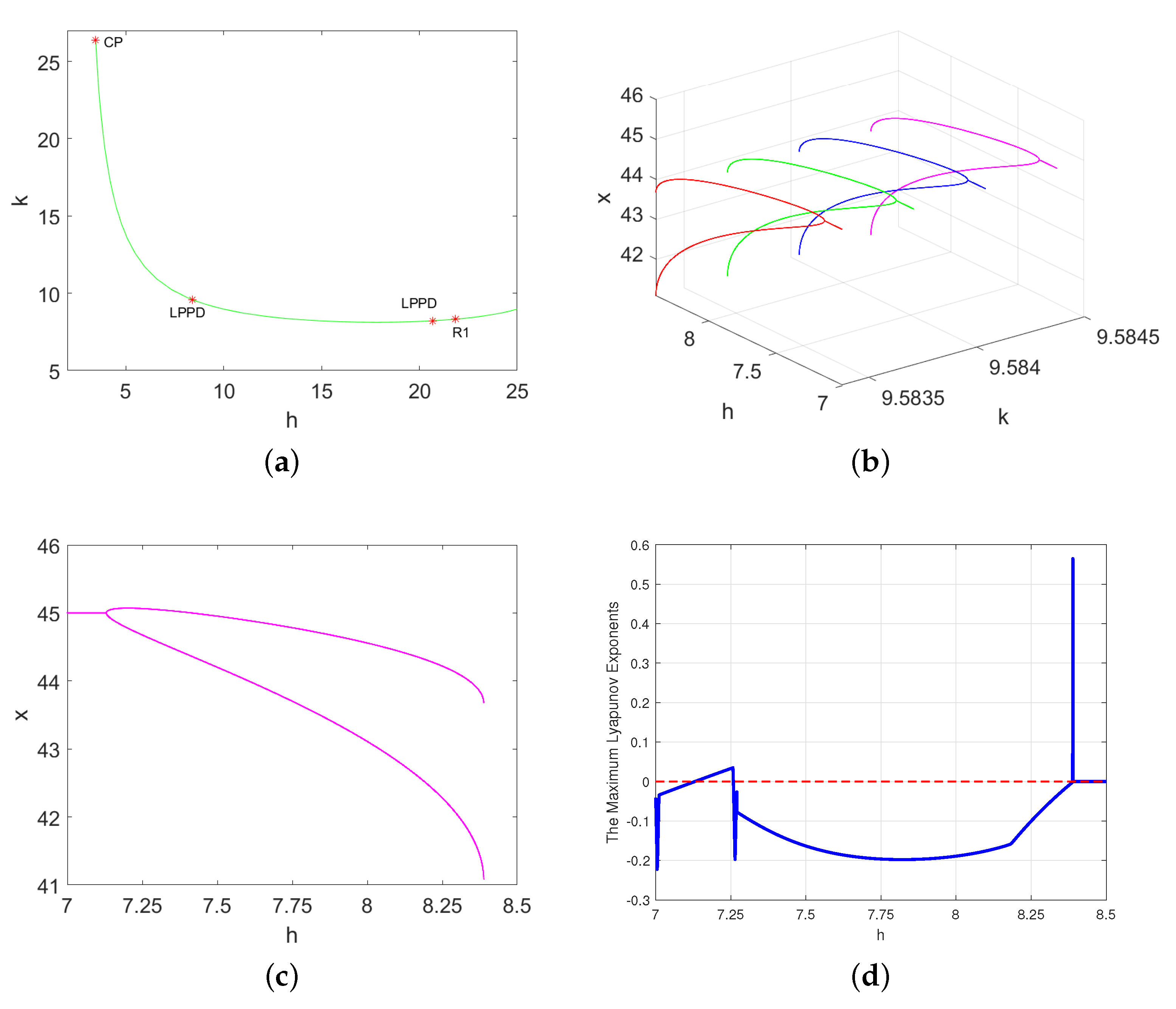
Theorem 1.

If h and k are chosen as two bifurcation parameters, then model (3) undergoes a fold-flip bifurcation at $E^{\ast }$ when the parameters $h,k$ vary in a sufficiently small neighborhood of $(h_f^{\ast },k_f^{\ast })$ near the $E^{\ast }$ with (19) and (22) hold. Moreover, the model (3) has the following local codimension-one bifurcation behaviors:

(I) 

There is a non-degenerate fold bifurcation curve, fold: $({\xi }_1,{\xi }_2,{\mu }_1)=(\frac{{\mu }_2}{{\sigma }_1\left(0\right)}+\mathcal{O}\left({\mu }_2^2\right),0$, $\frac{{\mu }_2^2}{2{\sigma }_1\left(0\right)+\mathcal{O}\left({\mu }_2^3\right)})$, if ${\sigma }_1\left(0\right)\ne 0$;

(II) 

There is a non-degenerate flip bifurcation curve, flip: $({\xi }_1,{\xi }_2,{\mu }_1)=(0,0,0)$, if ${\sigma }_2\left(0\right)\ne 0$;

(III) 

There is a non-degenerate Neimark–Sacker bifurcation curve, NS: $({\xi }_1,{\xi }_2,{\mu }_2)=\left(0,\sqrt{-\frac{2{\mu }_1}{{\sigma }_2\left(0\right)}}\right.\left.+\mathcal{O}\left({\mu }_1^{\frac{2}{3}}\right),\phantom{\mathcal{O}\left({\mu }_1^{\frac{2}{3}}\right)}\frac{({\sigma }_4\left(0\right)+2{\sigma }_2\left(0\right)){\mu }_1}{{\sigma }_2\left(0\right)}+\mathcal{O}\left({\mu }_1^2\right)\right)$, if ${\sigma }_2\left(0\right)>0$ and ${\mu }_1<0$.

3.2. 1:3 Resonance

In this subsection, we will consider codimension-two bifurcation with 1:3 resonance in model (3). Model (3) has a pair of complex conjugate multiples, which are denoted by ${\lambda }_{R_3}=-\frac{1}{2}+\frac{\sqrt{3}\mathrm{i}}{2}$ and ${\overline{\lambda }}_{R_3}=-\frac{1}{2}-\frac{\sqrt{3}\mathrm{i}}{2}$, if

$$\left\{\begin{array}{c}\mathcal{N}(x,y,\vartheta )-{(x,y)}^T={(0,0)}^T,\hfill \\ det\left(J\right(x,y,\vartheta \left)\right)-1=0,\hfill \\ \mathrm{trace}\left(J\right(x,y,\vartheta \left)\right)-1=0.\hfill \end{array}\right.$$

(25)

The exact solution $(x,y,h,k)$ of (25) is denoted by $(x^{\ast },y^{\ast },h_{R_3},k_{R_3})$. Therefore, model (3) may undergo a codimension-two bifurcation with 1:3 resonance at $E^{\ast }$ when the bifurcation parameters $h=h_{R_3}$ and $k=k_{R_3}$. Letting $u\left(n\right)=x\left(n\right)-x^{\ast }$ and $v\left(n\right)=y\left(n\right)-y^{\ast }$, model (3) can be transformed into the following form with Taylor expansion at the origin $(0,0)$

$$\left\{\begin{array}{c}{u}_{n+1}=\left(1-m(h,k)\right)u_n-p(h,k)v_n+F_{R_3}(u_n,v_n)+\mathcal{O}\left(|u_n,v_n{|}^4\right),\hfill \\ v_{n+1}=q(h,k)u_n+\left(1+n(h,k)\right)v_n+G_{R_3}(u_n,v_n)+\mathcal{O}\left(|u_n,v_n{|}^4\right),\hfill \end{array}\right.$$

(26)

where

$$F_{R_3}(u_n,v_n)=\sum _{2⩽i+j⩽3}{c}_{ij}{u}_n^i{v}_n^j,G_{R_3}(u_n,v_n)=\sum _{2⩽i+j⩽3}{d}_{ij}{u}_n^i{v}_n^j,$$

with

$$\begin{array}{cc}\hfill & m(h,k)=h\left(\frac{\beta y^{\ast }}{k+y^{\ast }}+\mu \right),n(h,k)=h\left(\frac{\beta k{x}^{\ast }}{{(k+y^{\ast })}^2}-\frac{({\alpha }_1-{\alpha }_0)b^2}{{(b+y^{\ast })}^2}-{\alpha }_0-\gamma -\mu \right),p(h,k)=\frac{\beta hk{x}^{\ast }}{{(k+y^{\ast })}^2},\hfill \\ \hfill & q(h,k)=\frac{\beta h{y}^{\ast }}{k+y^{\ast }},c_{11}=-\frac{h\beta k}{{(k+y^{\ast })}^2},c_{02}=\frac{h\beta k{x}^{\ast }}{{(k+y^{\ast })}^3},c_{12}=\frac{h\beta k}{{(k+y^{\ast })}^3},c_{03}=-\frac{h\beta k{x}^{\ast }}{{(k+y^{\ast })}^4},d_{11}=-\frac{h\beta k}{{(k+y^{\ast })}^2},\hfill \\ \hfill & d_{02}=h\left(\frac{({\alpha }_1-{\alpha }_0)b^2}{{(b+y^{\ast })}^3}-\frac{\beta k{x}^{\ast }}{{(k+y^{\ast })}^3}\right),d_{12}=-\frac{h\beta k}{{(k+y^{\ast })}^3},d_{03}=h\left(\frac{\beta k{x}^{\ast }}{{(k+y^{\ast })}^4}-\frac{({\alpha }_1-{\alpha }_0)b^2}{{(b+y^{\ast })}^4}\right),\hfill \\ \hfill & c_{30}=c_{21}=c_{20}=0,d_{30}=d_{21}=d_{20}=0.\hfill \end{array}$$

By (26), the Jacobian matrix of $E^{\ast }$ is obtained by

$$J_{E^{\ast }}(h,k)=\left(\begin{array}{cc}1-m(h,k)& -p(h,k)\\ q(h,k)& 1+n(h,k)\end{array}\right).$$

We denote $J^{\ast }=J_{E^{\ast }}(h_{R_3},k_{R_3})$. There are eigenvector $q_{{}_{R_3}}$ and adjoint eigenvector $p_{{}_{R_3}}\in {\mathbb{C}}^2$, satisfying $J^{\ast }{q}_{{}_{R_3}}={\lambda }_{R_3}{q}_{{}_{R_3}}$ $J^{\ast T}{p}_{{}_{R_3}}={\overline{\lambda }}_{R_3}{p}_{{}_{R_3}}$, $⟨p_{{}_{R_3}},q_{{}_{R_3}}⟩=1$, where ${\lambda }_{R_3}=-\frac{1}{2}+\frac{\sqrt{3}\mathrm{i}}{2}$, $q_{{}_{R_3}}={\left(q_{{}_{R_{3,1}}}{q}_{{}_{R_{3,2}}}\right)}^T={\left(-p(h_{R_3},k_{R_3})-\frac{3}{2}+\frac{\sqrt{3}\mathrm{i}}{2}+m(h_{R_3},k_{R_3})\right)}^T$, and $p_{{}_{R_3}}={(p_{{}_{R_{3,1}}},p_{{}_{R_{3,2}}})}^T={\left(q(h_{R_3},k_{R_3}),-\frac{3}{2}+\frac{\sqrt{3}\mathrm{i}}{2}+m(h_{R_3},k_{R_3})\right)}^T$.

Now, any vector $U={(u,v)}^T\in {\mathbb{R}}^2$ can be represented in the form $U=z{q}_{{}_{R_3}}+\overline{z}{\overline{q}}_{{}_{R_3}}$, where ${\overline{p}}_{{}_{R_3}}=({\overline{p}}_{{}_{R_{3,1}}},{\overline{p}}_{{}_{R_{3,2}}})$, and ${\overline{q}}_{{}_{R_3}}=({\overline{q}}_{{}_{R_{3,1}}},{\overline{q}}_{{}_{R_{3,2}}})$ are the conjugates of $p_{{}_{R_3}}$ and $q_{{}_{R_3}}$, respectively. Hence, model (26) can be written in the complex form

$$\left(\begin{array}{c}{z}_{n+1}\\ {\overline{z}}_{n+1}\end{array}\right)=\left(\begin{array}{cc}{\lambda }_{R_3}& 0\\ 0& {\overline{\lambda }}_{R_3}\end{array}\right)\left(\begin{array}{c}{z}_n\\ {\overline{z}}_n\end{array}\right)+\left(\begin{array}{c}{\displaystyle \sum _{2⩽i+j⩽3}}{g}_{ij}{z}_n^i{\overline{z}}_n^j+\mathcal{O}\left(|z_n,{\overline{z}}_n{|}^4\right)\\ {\displaystyle \sum _{2⩽i+j⩽3}}{\overline{g}}_{ij}{z}_n^i{\overline{z}}_n^j+\mathcal{O}\left(|z_n,{\overline{z}}_n{|}^4\right)\end{array}\right),$$

(27)

where $g_{ij}$ is given in Appendix B, and ${\overline{g}}_{ij}$ is the complex conjugate of $g_{ij}$. Now, what we need to study is

$$z_{n+1}={\lambda }_{R_3}{z}_n+\sum _{2⩽i+j⩽3}{g}_{ij}{z}_n^i{\overline{z}}_n^j+\mathcal{O}\left(|z_n,{\overline{z}}_n{|}^4\right),$$

(28)

since the second component of (27) is simply the complex conjugate of the first component.

Some quadratic terms can be eliminated by the following transformation

$$z_n=w_n+\frac{l_{20}}{2}{w}_n^2+l_{11}{w}_n{\overline{w}}_n+\frac{l_{02}}{2}{\overline{w}}_n^2,$$

(29)

where $l_{20},l_{11}$, and $l_{02}$ are certain unknown functions. Using (29) and its inverse transformation, model (28) can be rewritten in the following form

$$w_{n+1}={\lambda }_{R_3}{w}_n+\sum _{2⩽i+j⩽3}{s}_{ij}{w}_n^i{\overline{w}}_n^j+\mathcal{O}\left(|w_n,{\overline{w}}_n{|}^4\right),$$

(30)

where $s_{ij}$ is given in Appendix B.

The coefficients in front of the $w^{2\_}$ and $w{\overline{w}}^{\_}$ terms are eliminated by setting

$$l_{20}=-\frac{2g_{20}}{\sqrt{3}\mathrm{i}},l_{11}=\frac{2g_{11}}{3-\sqrt{3}\mathrm{i}},l_{02}=0.$$

Hence, (30) becomes

$$w_{n+1}={\lambda }_{R_3}{w}_n+g_{20}{\overline{w}}_n^2+\sum _{i+j=3}{s}_{ij}{w}_n^i{\overline{w}}_n^j+\mathcal{O}\left(|w_n,{\overline{w}}_n{|}^4\right).$$

(31)

The next step is to annihilate cubic terms by applying an invertible smooth transformation

$$w_n={\varphi }_n+\frac{l_{30}}{6}{\varphi }_n^3+\frac{l_{12}}{2}{\varphi }_n{\overline{\varphi }}_n^2+\frac{l_{03}}{6}{\overline{\varphi }}_n^3.$$

(32)

Using (32) and its inverse transformation, model (31) can be rewritten in the following form

$${\varphi }_{n+1}={\lambda }_{R_3}{\varphi }_n+g_{20}{\overline{\varphi }}_n^2+\sum _{i+j=3}{t}_{ij}{\varphi }_n^i{\overline{\varphi }}_n^j+\mathcal{O}\left(|{\varphi }_n,{\overline{\varphi }}_n{|}^4\right),$$

(33)

where

$$t_{30}=s_{{}_{30}}-\frac{3-\sqrt{3}\mathrm{i}}{12}{l}_{30},t_{21}=s_{{}_{21}},t_{12}=s_{{}_{12}}+\frac{\sqrt{3}\mathrm{i}}{2}{l}_{12},t_{03}=s_{{}_{03}}-\frac{3-\sqrt{3}\mathrm{i}}{12}{l}_{03}.$$

Hence, the coefficients in front of the $w^{3\_}$, $w{\overline{w}}^{2\_}$, and ${\overline{w}}^{3\_}$ terms are eliminated by setting

$$l_{30}=\frac{12s_{{}_{30}}}{3-\sqrt{3}\mathrm{i}},l_{21}=0,l_{12}=-\frac{2s_{{}_{12}}}{\sqrt{3}\mathrm{i}},l_{03}=\frac{12s_{{}_{03}}}{3-\sqrt{3}\mathrm{i}}.$$

Finally, an approximating equation of (33) should have the following form

$${\varphi }_{n+1}={\lambda }_{R_3}{\varphi }_n+g_{02}{\overline{\varphi }}_n^2+t_{21}{\varphi }_n^2{\overline{\varphi }}_n+\mathcal{O}\left(|{\varphi }_n,{\overline{\varphi }}_n{|}^4\right).$$

(34)

According to Lemma 9.12 in [34], defining

$${\mathcal{B}}_1=-\frac{3(1+\sqrt{3}\mathrm{i})}{2}{g}_{02},{\mathcal{C}}_1=-3{\left|g_{02}\right|}^2-\frac{3(1+\sqrt{3}\mathrm{i})}{2}{t}_{21},$$

(35)

we can obtain the following theorem.

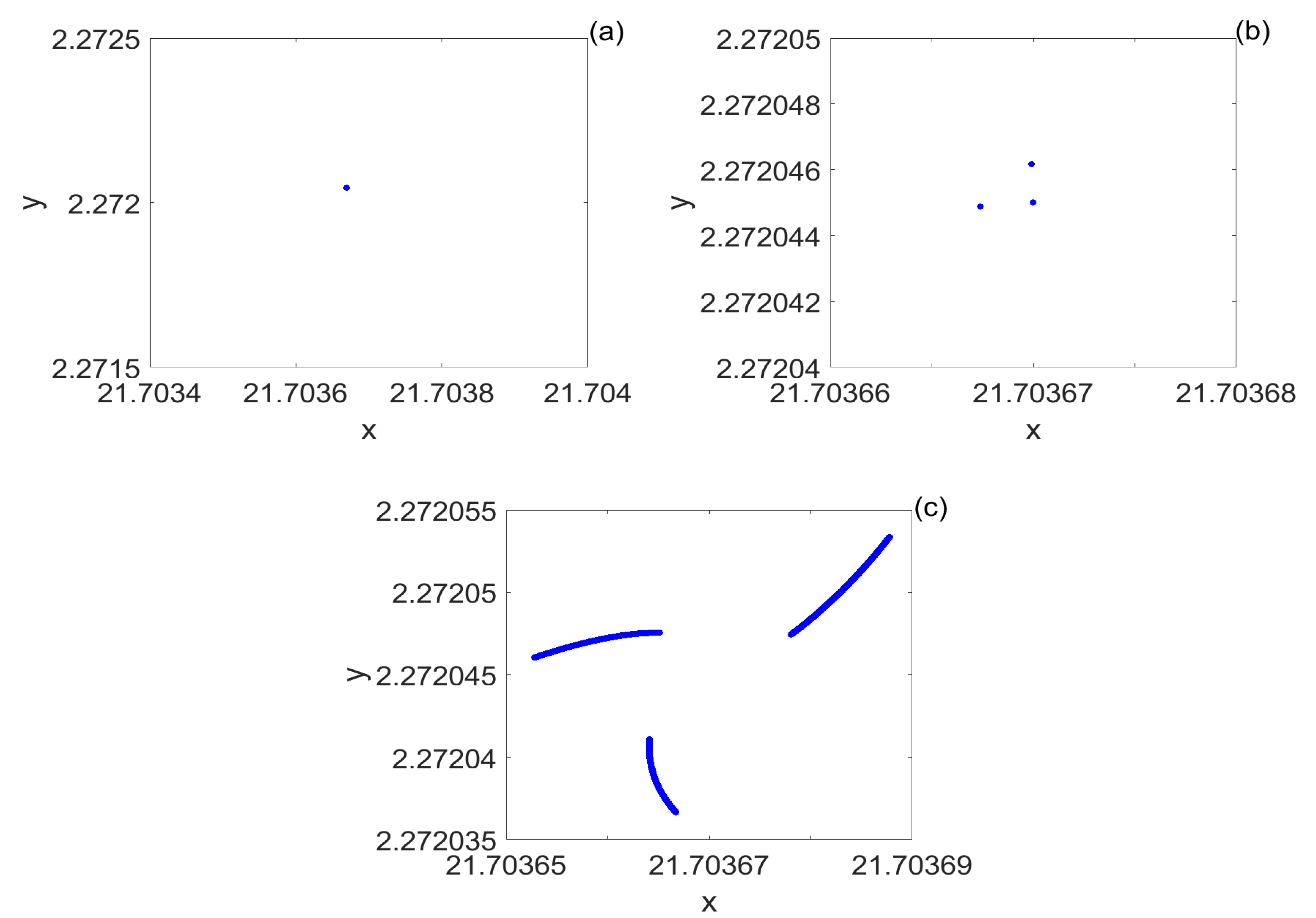
Theorem 2.

If h and k are chosen as two bifurcation parameters, then model (3) undergoes a codimension-two bifurcation with 1:3 resonance at $E^{\ast }$ when the conditions (25) and ${\mathcal{B}}_1\ne 0$, $\mathrm{Re}\left({\mathcal{C}}_1\right)\ne 0$ hold. $\mathrm{Re}\left({\mathcal{C}}_1\right)\ne 0$ determines the stability of the bifurcation invariant closed curve. Moreover, model (3) recognizes a few of the following complex codimension-one bifurcation curves:

(I) 

There is a non-degenerate Neimark–Sacker bifurcation at the trivial fixed point $E^{\ast }$ of (35);

(II) 

There is a saddle cycle of periodic three corresponding to the saddle fixed points $E^{\ast }$ of (35);

(III) 

There is a homoclinic structure formed by the stable and unstable invariant manifolds of the period three cycle intersecting transversally in an exponentially narrow parameter region.

3.3. 1:4 Resonance

In this subsection, we consider codimension-two bifurcation with 1:4 resonance in model (3). Model (3) has a pair of complex conjugate multiples, which are denoted by ${\lambda }_{R_4}=\mathrm{i}$ and ${\overline{\lambda }}_{R_4}=-\mathrm{i}$ if

$$\left\{\begin{array}{c}\mathcal{N}(x,y,\vartheta )-{(x,y)}^T={(0,0)}^T,\hfill \\ det\left(J\right(x,y,\vartheta \left)\right)-1=0,\hfill \\ \mathrm{trace}\left(J\right(x,y,\vartheta \left)\right)=0.\hfill \end{array}\right.$$

(36)

The exact solution $(x,y,h,k)$ of model (36) is denoted by $(x^{\ast },y^{\ast },h_{R_4},k_{R_4})$. Therefore, model (3) may undergo a codimension-two bifurcation with 1:4 resonance at $E^{\ast }$ when the bifurcation parameters $h=h_{R_4}$ and $k=k_{R_4}$. Similar to the previous subsection, the Jacobian matrix of $E^{\ast }$ is given by $J_{E^{\ast }}(h,k)=\left(\begin{array}{cc}1-m(h,k)& -p(h,k)\\ q(h,k)& 1+n(h,k)\end{array}\right).$ We denote $J^{\ast }=J_{E^{\ast }}(h_{R_4},k_{R_4})$. There are eigenvector $q_{{}_{R_4}}$ and adjoint eigenvector $p_{{}_{R_4}}\in {\mathbb{C}}^2$, satisfying $J^{\ast }{q}_{{}_{R_4}}={\lambda }_{R_4}{q}_{{}_{R_4}}$, $J^{\ast T}{p}_{{}_{R_4}}={\overline{\lambda }}_{R_4}{p}_{{}_{R_4}}$, $⟨p_{{}_{R_4}},q_{{}_{R_4}}⟩=1$, where ${\lambda }_{R_4}=\mathrm{i}$, $q_{{}_{R_4}}={(q_{{}_{R_{4,1}}},q_{{}_{R_{4,2}}})}^T=(-p(k_{R_4},h_{R_4})$, $m(h_{R_4},k_{R_4}){-1+\mathrm{i})}^{\mathrm{T}}$, $p_{{}_{R_4}}={(p_{{}_{R_{4,1}}},p_{{}_{R_{4,2}}})}^T={\left(-\frac{q(h_{R_4},k_{R_4})}{2},-\frac{m(h_{R_4},k_{R_4})-1-\mathrm{i}}{2}\right)}^T$. Now, any vector $U={(u,v)}^T\in {\mathbb{R}}^2$ can be represented in the form $U=z{q}_{{}_{R_4}}+\overline{z}{\overline{q}}_{{}_{R_4}}$, where ${\overline{q}}_{{}_{R_4}}$ is the conjugate of $q_{{}_{R_4}}$. Hence, model (26) can be written in the complex form

$$z_{n+1}={\lambda }_{R_4}{z}_n+\sum _{2⩽i+j⩽3}{g}_{ij}{z}_n^i{\overline{z}}_n^j+\mathcal{O}\left(|z_n,{\overline{z}}_n{|}^4\right),$$

(37)

where ${\lambda }_{R_4}=\mathrm{i}$ and $g_{ij}(2⩽i+j⩽3)$ are defined as in Appendix B with $q_{{}_{R_3,1}}$, $q_{{}_{R_3,2}}$, $p_{{}_{R_3,1}}$, and $p_{{}_{R_3,2}}$ replaced by $q_{{}_{R_{4,1}}}$, $q_{{}_{R_{4,2}}}$, $p_{{}_{R_{4,1}}}$, and $p_{{}_{R_{4,2}}}$, respectively. Using (29) and its inverse transformation, model (37) can be rewritten in the following form

$$w_{n+1}={\lambda }_{R_4}{w}_n+\sum _{2⩽i+j⩽3}{\tilde{s}}_{ij}{w}_n^i{\overline{w}}_n^j+\mathcal{O}\left(|w_n,{\overline{w}}_n{|}^4\right),$$

(38)

where ${\tilde{s}}_{ij}$ are given in Appendix C.

All the quadratic terms are eliminated by setting

$$l_{20}=-\frac{2g_{20}}{1+\mathrm{i}},l_{11}=\frac{g_{11}}{1-\mathrm{i}},l_{02}=-\frac{2g_{02}}{1+\mathrm{i}}.$$

Hence, (38) becomes

$$w_{n+1}={\lambda }_{R_4}{w}_n+\sum _{i+j=3}{\tilde{s}}_{ij}{w}_n^i{\overline{w}}_n^j+\mathcal{O}\left(|w_n,{\overline{w}}_n{|}^4\right).$$

(39)

Using (32) and its inverse transformation, model (39) can be rewritten in the following form

$${\varphi }_{n+1}={\lambda }_{R_4}{\varphi }_n+\sum _{i+j=3}{\tilde{t}}_{ij}{\varphi }_n^i{\overline{\varphi }}_n^j+\mathcal{O}\left(|{\varphi }_n,{\overline{\varphi }}_n{|}^4\right),$$

(40)

in which

$${\tilde{t}}_{30}={\tilde{s}}_{30}+\frac{\mathrm{i}}{3}{l}_{30},{\tilde{t}}_{21}={\tilde{s}}_{21},{\tilde{t}}_{12}={\tilde{s}}_{12}+\mathrm{i}{l}_{12},{\tilde{t}}_{03}={\tilde{s}}_{03}.$$

Hence, the coefficients in front of the $w^{3\_}$ and $w{\overline{w}}^{2\_}$ terms are eliminated by setting

$$l_{30}=\frac{12{\tilde{s}}_{30}}{3-\sqrt{3}\mathrm{i}},l_{21}=0,l_{12}=-\frac{2{\tilde{s}}_{12}}{\sqrt{3}\mathrm{i}},l_{03}=0.$$

Finally, an approximating equation of (40) should have the following form

$${\varphi }_{n+1}={\lambda }_{R_4}{\varphi }_n+{\tilde{t}}_{21}{\varphi }_n^2{\overline{\varphi }}_n+{\tilde{t}}_{03}{\overline{\varphi }}_n^3+\mathcal{O}\left(|{\varphi }_n,{\overline{\varphi }}_n{|}^4\right).$$

(41)

According to Lemma 9.14 in [34], defining

$${\mathcal{B}}_2=-2\mathrm{i}{\tilde{t}}_{21},{\mathcal{C}}_2=-\frac{2\mathrm{i}}{3}{\tilde{t}}_{03},$$

(42)

if ${\mathcal{C}}_2\ne 0$, letting

$$\mathcal{D}=\frac{{\mathcal{B}}_2}{|{\mathcal{C}}_2|},$$

(43)

we can obtain the following theorem.

Theorem 3.

If h and k are chosen as two bifurcation parameters, then model (3) undergoes a codimension-two bifurcation with 1:4 resonance at $E^{\ast }$ when the conditions (36) and ${\mathcal{C}}_2\ne 0$, $\mathrm{Re}\left(\mathcal{D}\right)\ne 0$, and $\mathrm{Im}\left(\mathcal{D}\right)\ne 0$ hold.

4. Numerical Bifurcation Analysis

In this section, the phase portraits, bifurcation diagrams, maximum Lyapunov exponents diagrams, and the diagrams of local attraction basins in the neighborhood of fixed points for model (3) are presented to verify the correctness of the analytical results established in Theorems 1–3 by using the MATLAB and the MATLAB package MatcontM [35,36,37,38]. Let $A=2.25,\beta =0.1,{\alpha }_1=0.5,{\alpha }_0=0.2,\gamma =0.2,b=0.6$, and $\mu =0.05$ for model (3) in the following Section 4.1, Section 4.2 and Section 4.3.

4.1. Fold-Flip Bifurcation

For Equation (11), we obtain one of its exact solutions $(x^{\ast },y^{\ast },h_f^{\ast },k_f^{\ast })=(43.664637,$ $0.908638, 8.388521, 9.58437)$. Therefore, model (3) may undergo a fold-flip bifurcation at the fixed point $E^{\ast }(x^{\ast },y^{\ast })=(43.664637,0.908638)$ when the critical parameter values $h_f^{\ast }=8.388521, k_f^{\ast }=9.58437$. The eigenvalues are ${\lambda }_{1,2}=\pm 1$ and ${\overline{a}}_{11}=0.259668\ne 0,det\frac{\partial \Gamma }{\partial (\tilde{X},\varphi )}{|}_{(\tilde{X}=\varphi =0)}=0.0224769\ne 0$. According to Theorem 1, it means that model (3) undergoes a fold-flip bifurcation at $E^{\ast }(43.664637,0.908638)$.

The continuation of the fold bifurcation curve for two control parameters k and h is drawn in Figure 1a. Two fold-flip (LPPD) bifurcation points are detected. Meanwhile, a cusp (CP) and 1:1 resonance (R1) bifurcation points also are detected. Figure 1b presents a three-dimensional bifurcation diagram in $(k,h,x)$ space near $E^{\ast }(43.664637,0.908638)$ when k and h vary in the neighborhood of $(h_f^{\ast },k_f^{\ast })=(8.388521,9.58437)$, which is the left LPPD point in Figure 1a. Figure 1c depicts a two-dimensional bifurcation diagram in $(h,x)$ plane for $h\in [7,8.5]$ when $k=k_f^{\ast }=9.58437$. The maximum Lyapunov exponents diagram corresponding to Figure 1c is drawn in Figure 1d.

Figure 1. (a) The continuation curve of the LP point consists of fold-flip (LPPD), cusp (CP), and resonance 1:1 (R1) bifurcation points in $(k,h)$ plane. (b) Bifurcation diagram in three-dimensional $(k,h,x)$ space with the change of k and h. From left to right, the values of parameter k are $9.58337,9.58370,9.58404$, and $9.58437$, respectively. (c) Fold-flip bifurcation diagram in $(h,x)$ plane with $k=9.58437$ and $h\in [7,8.5]$. (d) The maximum Lyapunov exponents diagram corresponding to (c).

4.2. 1:3 Resonance

For Equation (25), we obtain one of its exact solutions $(x^{\ast },y^{\ast },h_{R_3},k_{R_3})=(21.70367$, $2.272045,9.112002,1.961387)$. Therefore, model (3) may undergo a 1:3 resonance at the fixed point $E^{\ast }(x^{\ast },y^{\ast })=(21.70367,2.272045)$ when the critical parameter values $h_{R_3}=9.112002$, and $k_{R_3}=1.961387$. The eigenvalues are ${\lambda }_{1,2}=-0.5\pm 0.8660254\mathrm{i}$ and ${\mathcal{B}}_1=-0.556655-0.2653575\mathrm{i}\ne 0$, ${\mathcal{C}}_1=275.6926179-1616.468972\mathrm{i}$, and $\mathrm{Re}\left({\mathcal{C}}_1\right)=275.6926179\ne 0$. According to Theorem 2, it means that model (3) undergoes a codimension-two bifurcation with 1:3 resonance at $E^{\ast }(21.70367,2.272045)$.

The 1:3 resonance bifurcation point is detected in the continuation of the Neimark–Sacker curve, which is drawn in Figure 2a. Figure 2b presents a three-dimensional bifurcation diagram in $(k,h,x)$ space near $E^{\ast }(21.70367,2.272045)$ when k and h vary in a neighborhood of $(h_{R_3},k_{R_3})=(9.112002,1.961387)$. Figure 2c depicts a 2-dimensional bifurcation diagram in $(h,x)$ plane when $k=k_{R_3}=1.961387$. The local amplification of Figure 2c for $h\in [9.11,9.1145]$ is obtained in Figure 2d. The maximum Lyapunov exponents diagram, which corresponds to Figure 2c is drawn in Figure 2e. The maximum Lyapunov exponents are negative when $h<h_{R_3}=9.112002$. There is a stable fixed point for each h. However, the maximum Lyapunov exponents are positive when $h>h_{R_3}=9.112002$, which means model (3) has chaotic behavior near the 1:3 resonance point $E^{\ast }(21.70367,2.272045)$. The phase portraits for different values of h corresponding Figure 2c are drawn in Figure 3.

Figure 2. (a) The continuation curve of the Neimark–Sacker point contains Chenciner (CH) bifurcation, resonance 1:2 (R2), resonance 1:3 (R3), and resonance 1:4 (R4) points in $(h,k)$ plane. (b) Bifurcation diagram in three-dimensional $(k,h,x)$ space with the change of k and h. The values of parameter k are $1.960387,1.960720,1.960985$, and $1.961387$ from left to right. (c) 1:3 resonance bifurcation diagram in $(h,x)$ plane when $k=1.961387$ and $h\in [9.106,9.1145]$. (d) Local amplification corresponding to (c) for $h\in [9.11,9.1145]$. (e) The maximum Lyapunov exponents diagram corresponding to (c).

Figure 3. Phase portraits for different values of h corresponding to Figure 3c. (a) A stable fixed point for $h=9.106$. (b) Phase portrait of period-3 for $h=9.112$. (c) Phase portrait of 1:3 resonance for $h=9.113$.

4.3. 1:4 Resonance

For Equation (36), we obtain one of its exact solutions $(x^{\ast },y^{\ast },h_{R_4},k_{R_4})=(26.348645$, $1.773490,9.309313,3.237305)$. Therefore, model (3) may undergo a 1:4 resonance at the fixed point $E^{\ast }(x^{\ast },y^{\ast })=(26.348645,1.773490)$ when the critical parameter values $h_{R_4}=9.309313$, and $k_{R_4}=3.237305$. The eigenvalues are ${\lambda }_{1,2}=\pm \mathrm{i}$ and ${\mathcal{B}}_2=-0.5463087328-0.7196720302\mathrm{i}$, ${\mathcal{C}}_2=0.3523986225-0.2941681928\mathrm{i}\ne 0$, $\mathcal{D}=-1.190105762-1.56776888\mathrm{i}$, $\mathrm{Re}\left(\mathcal{D}\right)=-1.190105762\ne 0$, and $\mathrm{Im}\left(\mathcal{D}\right)=-1.567768880\ne 0$. According to Theorem 3, it means that model (3) undergoes a codimension-two bifurcation with 1:4 resonance at $E^{\ast }(26.348645,1.773490)$.

The 1:4 resonance bifurcation point has been detected in the continuation of the Neimark–Sacker curve, which is drawn in Figure 2a. Figure 4a presents a three-dimensional bifurcation diagram in $(k,h,x)$ space near $E^{\ast }(26.348645,1.773490)$ when k and h vary in the neighborhood of $h_{R_4}=9.309313$, and $k_{R_4}=3.237305$, which is the R4 point in Figure 2a. Figure 4b depicts a two-dimensional bifurcation diagram in $(h,x)$ plane for $h\in [9.308,9.316]$ when $k=k_{R_4}=3.237305$. The maximum Lyapunov exponents diagram corresponding to Figure 4b is drawn in Figure 4c. The maximum Lyapunov exponents are negative when $h<h_{R_4}=9.309313$. There is(are) stable fixed point(s) for each h. However, some maximum Lyapunov exponents are positive when $h>h_{R_4}=9.309313$, which means model (3) has chaotic behavior near the resonance 1:4 point $E^{\ast }(26.348645,1.773490)$. Phase portraits for different values of h corresponding to Figure 4b are drawn in Figure 5.

Figure 4. (a) Bifurcation diagram in three-dimensional $(k,h,x)$ space with the change of k and h. The values of parameter k are $3.237305$, $3.237338$, $3.237371$, and $3.237405$ from left to right. (b) 1:4 resonance bifurcation diagram in $(h,x)$ plane with $k=3.237305$ and $h\in [9.308,9.316]$. (c) The maximum Lyapunov exponents diagram corresponding to (b).

Figure 5. Phase portraits for different values of h corresponding to Figure 4b. (a) A stable fixed point for $h=9.308$. (b) Phase portrait of period-4 for $h=9.3095$. (c) Phase portrait of 1:4 resonance for $h=9.312$. (d) Phase portrait of 1:4 resonance for $h=9.314$. (e) Chaotic attractor for $h=9.316$.

4.4. Local Attraction Basins Diagrams

To better demonstrate the dynamic behavior of the system from a more classical perspective, the problem of the attraction basins of fixed points is discussed. The attraction basin of an attractor is the set containing initial points, i.e., the trajectories from the start of this set all converge toward the attractor when $t\to \infty$ [42]. Generally, the attraction basin of an attractor is not a regular shape but is very complex. There are boundaries between the attraction basins of different attractors. Near the border, a slight change in the initial conditions will lead to entirely different results.

According to Lemma 1, we know that $C_1>0$, $C_2<0$, $C_3>0$, and $\Delta >0$ for $k=8,b=0.06$, and other parameters fixed as $A=2.25$, $\beta =0.1$, ${\alpha }_1=0.5$, ${\alpha }_0=0.2$, $\gamma =0.2$, $\mu =0.05$, and $h=6$; that is, model (3) has three fixed points, two of them are positive nontrivial fixed points, a spiral sink point $E_1(41.087,0.4)$ and a saddle point $E_2(43.2353,0.16667)$; the other is a stable node $E_0(45,0)$. When the value of h is increased or decreased, the number of fixed points of model (3) and the shape of the attraction basins of different fixed points will change greatly. To study the effect of the integral step size h on the discrete-time model, the local attraction basins of the corresponding continuous system (2) are exhibited in Figure 6. The local attraction basins in the $x\left(0\right)-y\left(0\right)$ plane are shown in Figure 7 for nine values of h in model (3).

Figure 6. The local attraction basin of system (2) in the $S\left(0\right)-I\left(0\right)$ initial plane. The blue region is the attraction basins of the equilibrium $E_1$, and the yellow region is for $E_0$, where $E_2$ is a saddle point.

Figure 7. For different values of the integral step size h, the local attraction basins in the $x\left(0\right)-y\left(0\right)$ initial plane are presented. (a) $h=0.01$. (b) $h=8$. (c) $h=10$. (d) $h=16$. (e) $h=17$. (f) $h=26$. (g) $h=27.4$. (h) $h=33$. (i) $h=36.3$. The blue regions are the attraction basins of the equilibrium $E_1$, and the yellow regions are for $E_0$, where $E_2$ is a saddle point. The cyanine regions are the attraction basins of the attracting invariant cycle, and the red regions are for the divergence.

With the variation in the parameters, it is obvious that a Neimark–Sacker bifurcation may occur around $E_1$ when $h=27.003451$ and the coefficient of the normal form is $-0.1615609$. Figure 7 shows the evolution of the local attraction basin of each fixed point with the change in the parameter h. Figure 7 shows some cases of the coexistence of the bistability states of model (3), such as the coexistence of two stable fixed points or the coexistence of a stable fixed point and an attracting invariant cycle. When $h>27.003451$, an attracting invariant cycle appears. The attraction basin of the fixed point $E_0$ becomes smaller and smaller throughout the whole evolution process. Comparing Figure 6 and Figure 7, we know that the dynamic behavior of model (3) is consistent with that of model (2) when the value of the integral step size h of model (3) is very small. However, the dynamic behaviors of model (2) and model (3) are very different as h becomes larger.

5. Conclusions

In this paper, we discussed codimension-two bifurcations of a simplified discrete-time SIR model with nonlinear incidence and recovery rates. From the perspective of infectious disease, the incidence and recovery rates are two important measurement indicators to detect the pathogenesis of infectious diseases and to prevent and control the speed of the spread of diseases. They are also important indicators reflecting the progress of national medical science and technology. We simplified system (1) to explore the impact of the intervention levels k and integral step size h on the dynamic behavior of the number of susceptible and infected individuals in the simplified discrete-time SIR model with nonlinear incidence and recovery rates. The results indicate that the codimension-two bifurcations of the discrete-time model can generate interesting and complex dynamic behaviors, such as chaos, which means that seemingly random irregular movements can occur in deterministic systems. However, in continuous systems, at least third-order differential equation systems can exhibit chaotic phenomena, such as the Lorentz system, whereas chaos can be demonstrated in low-order discrete-time systems. Hence, studying discrete-time systems can help us better explore some complex dynamics hidden in the continuous system.

Two approaches are used to localize the codimension-two bifurcation points. One is to calculate the parameter conditions for the existence of bifurcation with theoretical analysis, and the other is to draw the position of these points directly by numerical continuation. Fold-flip bifurcation and 1:3 and 1:4 resonances are analyzed theoretically in detail. 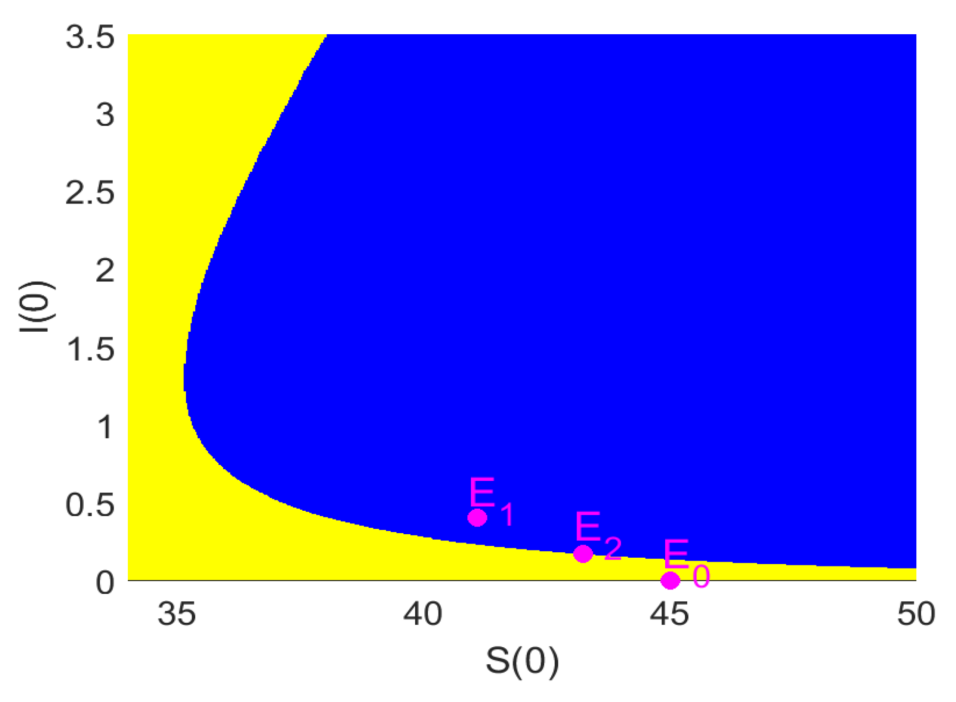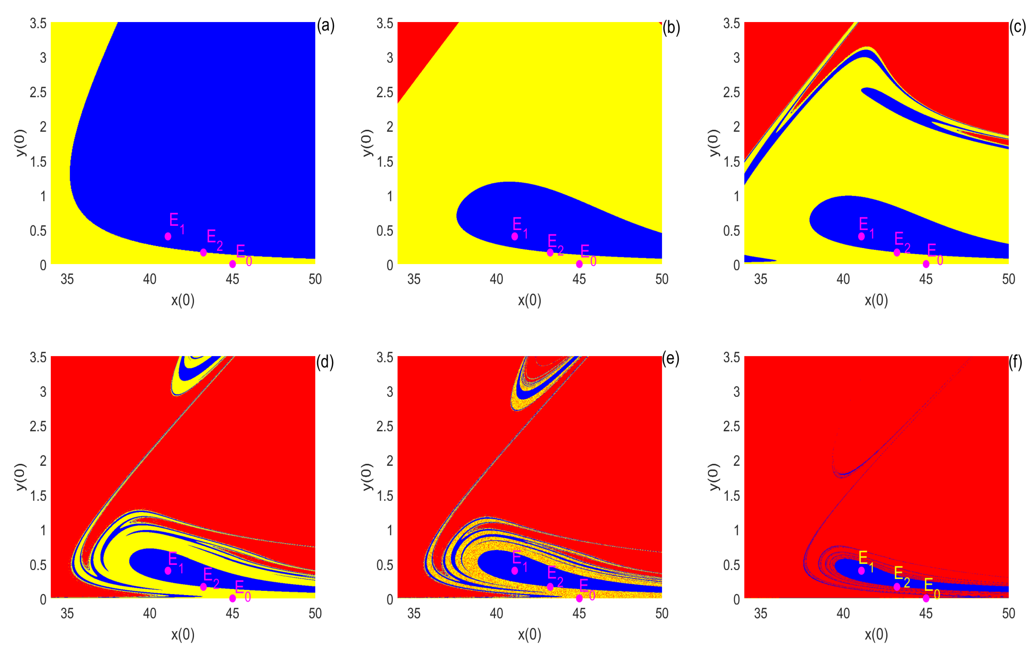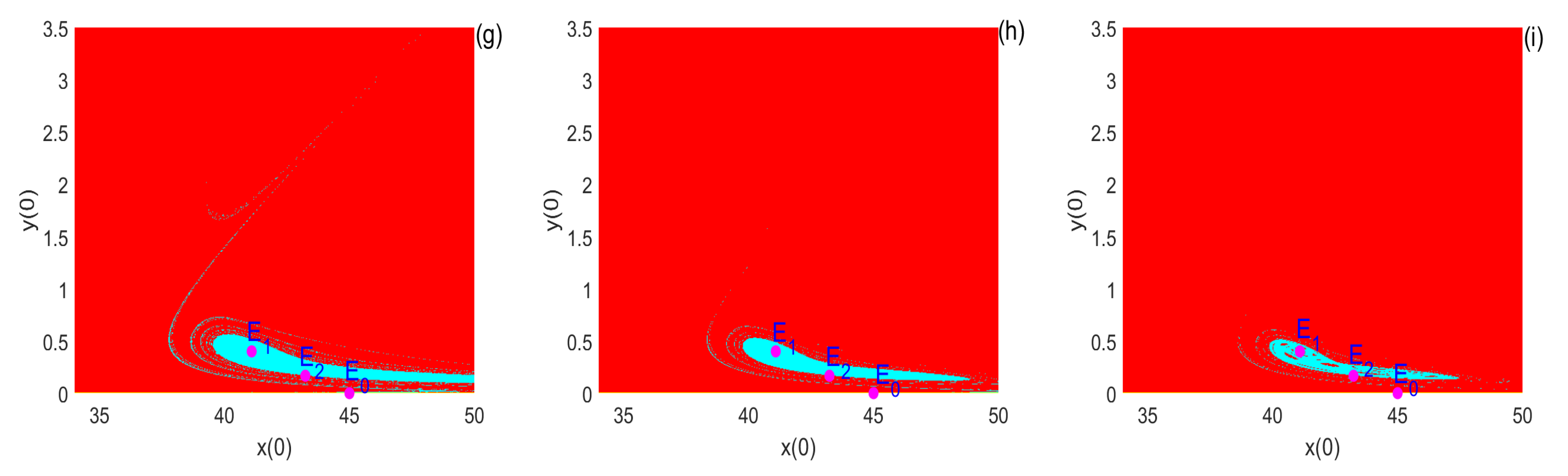A large number of numerical simulations have been used to test the correctness of the theoretical results and to demonstrate the rich dynamic behaviors in model (3). By contrasting the local attraction basins diagram at different integral step sizes of discrete-time model (3) with that of the corresponding continuous system, we can find that the dynamic behaviors of the discrete-time model and the corresponding continuous system are consistent when the integral step size is small. However, the discrete-time model can exhibit more complex dynamic behaviors, which have not been observed in the original continuous model for larger integral step sizes. That is to say, a discrete-time model can capture hidden dynamics that are not exhibited by the corresponding continuous model.

In this paper, we only conducted some basic research on the dynamic behavior of the simplified discrete-time SIR model. However, the model with higher dimensions may show higher codimension bifurcations. In addition, many influencing factors are time-varying, and the error between the study of non-autonomous systems and the actual situation may be smaller. It is very challenging to study these bifurcations and their practical applications. We leave these cases for future consideration.

References

- Mussap, C. The plague doctor of Venice. Int. Med. J. 2019, 49, 671–676. [Google Scholar] [CrossRef] [PubMed]
- Langa, J.; Sema, C.; Deus, N.; Colombo, M.; Taviani, E. Epidemic waves of cholera in the last two decades in Mozambique. J. Infect. Dev. Ctries. 2015, 9, 635–641. [Google Scholar] [CrossRef]
- Azizi, M.; Jalali, G.; Azizi, F. A history of the 1918 Spanish influenza pandemic and its impact on Iran. Arch. Iran. Med. 2010, 13, 262–265. [Google Scholar]
- Kermack, W.; Mckendrick, A. A contribution to the mathematical theory of epidemics. Proc. R. Soc. A 1927, 115, 700–721. [Google Scholar]
- Zhang, J.; Lou, H.; Ma, Z.; Wu, J. A compartmental model for the analysis of SARS transmission patterns and outbreak control measures in China. Appl. Math. Comput. 2005, 162, 909–924. [Google Scholar] [CrossRef] [PubMed]
- Yang, Y.; Li, W.; Zhu, L. The modeling and analysis of H1N1 influenza. Math. Pract. Theory 2011, 41, 11. [Google Scholar]
- Pájaro, M.; Fajar, N.; Alonso, A.; Otero-Muras, I. Stochastic SIR model predicts the evolution of COVID-19 epidemics from public health and wastewater data in small and medium-sized municipalities: A one year study. Chaos Solitons Fractals 2022, 164, 112671. [Google Scholar] [CrossRef]
- Hoque, M. An early estimation of the number of affected people in South Asia due to Covid-19 pandemic using susceptible, infected and recover model. Int. J. Mod. Phys. C 2020, 31, 2050140. [Google Scholar] [CrossRef]
- Ghosh, K.; Ghosh, A. Study of COVID-19 epidemiological evolution in India with a multi-wave SIR model. Nonlinear Dyn. 2022, 109, 47–55. [Google Scholar] [CrossRef]
- Gladkov, S. On the question of self-organization of population dynamics on Earth. Biophysics 2021, 66, 858–866. [Google Scholar] [CrossRef]
- Ma, L.; Hu, D.; Zheng, Z.; Ma, C.; Liu, M. Multiple bifurcations in a mathematical model of glioma-immune interaction. Commun. Nonlinear Sci. Numer. Simul. 2023, 123, 107282. [Google Scholar] [CrossRef]
- Zhang, X.; Wu, J.; Zhao, P.; Su, X.; Choi, D. Epidemic spreading on a complex network with partial immunization. Soft Comput. 2018, 22, 4525–4533. [Google Scholar] [CrossRef]
- Garg, H.; Nasir, A.; Jan, N.; Khan, S. Mathematical analysis of COVID-19 pandemic by using the concept of SIR model. Soft Comput. 2023, 27, 3477–3491. [Google Scholar] [CrossRef]
- Hossain, M.; Garai, S.; Jafari, S.; Pal, N. Bifurcation, chaos, multistability, and organized structures in a predator-prey model with vigilance. Chaos Interdiscip. J. Nonlinear Sci. 2022, 32, 063139. [Google Scholar] [CrossRef]
- Li, X.; Wang, W. A discrete epidemic model with stage structure. Chaos Solitions Fractals 2005, 26, 947–958. [Google Scholar] [CrossRef]
- Du, W.; Zhang, J.; Qin, S.; Yu, J. Bifurcation analysis in a discrete SIR epidemic model with the saturated contact rate and vertical transmission. J. Nonlinear Sci. Appl. 2016, 9, 4976–4989. [Google Scholar] [CrossRef]
- El-Shahed, M.; Abdelstar, I. Stability and bifurcation analysis in a discrete-time SIR epidemic model with fractional-order. Int. J. Nonlinear Sci. Numer. Simul. 2019, 20, 339–350. [Google Scholar] [CrossRef]
- Jang, S. Backward bifurcation in a discrete SIS model with vaccination. J. Biol. Syst. 2008, 16, 479–494. [Google Scholar] [CrossRef]
- Hu, D.; Cao, H. Bifurcation and chaos in a discrete-time predator-prey system of Holling and Leslie type. Commun. Nonlinear Sci. Numer. Simul. 2015, 22, 702–715. [Google Scholar] [CrossRef]
- Yu, Y.; Cao, H. Integral step size makes a difference to bifurcations of a discrete-time Hindmarsh-Rose model. Int. J. Bifurc. Chaos 2015, 25, 1550029. [Google Scholar] [CrossRef]
- Cheng, L.; Cao, H. Bifurcation analysis of a discrete-time ratio-dependent predator-prey model with Allee effect. Commun. Nonlinear Sci. Numer. Simul. 2016, 38, 288–302. [Google Scholar] [CrossRef]
- Liu, M.; Meng, F.; Hu, D. Codimension-one and codimension-two bifurcations of a discrete gene regulatory network. Nonlinear Dyn. 2022, 110, 1831–1865. [Google Scholar] [CrossRef]
- Eskandari, Z.; Alidousti, J. Stability and codimension 2 bifurcations of a discrete time SIR model. J. Frankl. Inst. 2020, 357, 10937–10959. [Google Scholar] [CrossRef]
- Li, B.; Liang, H.; He, Q. Multiple and generic bifurcation analysis of a discrete Hindmarsh-Rose model. Chaos Solitons Fractals 2021, 146, 110856. [Google Scholar] [CrossRef]
- Hu, Z.; Chang, L.; Teng, Z.; Chen, X. Bifurcation analysis of a discrete SIRS epidemic model with standard incidence rate. Adv. Differ. Equ. 2016, 2016, 155. [Google Scholar] [CrossRef]
- Marwan, M.; Ahmad, S. Bifurcation analysis for energy transport system and its optimal control using parameter self-tuning law. Soft Comput. 2020, 24, 17221–17231. [Google Scholar] [CrossRef]
- Chen, Q.; Teng, Z.; Wang, L.; Jiang, H. The existence of codimension-two bifurcation in a discrete SIS epidemic model with standard incidence. Nonlinear Dyn. 2013, 71, 55–73. [Google Scholar] [CrossRef]
- Chen, Q.; Teng, Z.; Wang, L. Codimension-two bifurcation analysis of a discrete predator-prey model with nonmonotonic functional response. J. Differ. Equ. Appl. 2017, 23, 2093–2115. [Google Scholar] [CrossRef]
- Liu, X.; Xiao, D. Complex dynamic behaviors of a discrete-time predator-prey system. Chaos Solitons Fractals 2017, 32, 80–94. [Google Scholar] [CrossRef]
- Alidousti, J.; Eskandari, Z.; Fardi, M.; Asadipour, M. Codimension two bifurcations of discrete Bonhoeffer-van der Pol oscillator model. Soft Comput. 2021, 25, 5261–5276. [Google Scholar] [CrossRef]
- Li, B.; He, Z. 1:2 and 1:4 resonance in a two-dimensional discrete Hindmarsh-Rose model. Nonlinear Dyn. 2015, 79, 705–720. [Google Scholar] [CrossRef]
- Marwan, M.; Mehbooband, M.; Ahmadand, S.; Aqeel, M. Hopf bifurcation of forced Chen system and its stability via adaptive control with arbitrary parameters. Soft Comput. 2020, 24, 4333–4341. [Google Scholar] [CrossRef]
- Eskandari, Z.; Alidousti, J.; Ghaziani, R. Codimension-one and -two bifurcations of a three-dimensional discrete game model. Int. J. Bifurc. Chaos 2021, 31, 2150023. [Google Scholar] [CrossRef]
- Kuznetsov, Y. Elements of Applied Bifurcation Theory, 2nd ed.; Springer: New York, NY, USA, 1998. [Google Scholar]
- Kuznetsov, Y.; Meijer, H. Numerical Bifurcation Analysis of Maps: From Theory to Software; Cambridge University Press: Cambridge, UK, 2019. [Google Scholar]
- Govaerts, W.; Kuznetsov, Y.; Ghaziani, R. Cl MatContM: A Toolbox for Continuation and Bifurcation of Cycles of Maps; Universiteit Gent: Ghent, Belgium; Utrecht University: Utrecht, The Netherlands, 2008. [Google Scholar]
- Neirynck, N.; Al-Hdaibat, B.; Govaerts, W.; Kuznetsov, Y.; Meijer, H. Using matcontm in the study of a nonlinear map in economics. J. Phys. Conf. Ser. 2016, 692, 012013. [Google Scholar] [CrossRef]
- Govaerts, W.; Khoshsiar, R.; Kuznetsov, Y.; Meijer, H. Numerical methods for two parameter local bifurcation analysis of maps. SIAM J. Sci. Comput. 2007, 29, 2644–2667. [Google Scholar] [CrossRef]
- Alshmmari, F.; Khan, M. Dynamic behaviors of a modified SIR model with nonlinear incidence and recovery rates. Alex. Eng. J. 2021, 60, 2997–3005. [Google Scholar] [CrossRef]
- Yu, X.; Liu, M.; Zheng, Z.; Hu, D. Complex dynamics of a discrete-time SIR model with nonlinear incidence and recovery rates. Int. J. Biomath. 2023, 16, 2250131. [Google Scholar] [CrossRef]
- Kuznetsov, Y.; Meijer, H.; Veen, L. The fold-flip bifurcation. Int. J. Bifurc. Chaos 2004, 14, 2253–2282. [Google Scholar] [CrossRef]
- Bao, B.; Chen, C.; Bao, H.; Zhang, X.; Xu, Q.; Chen, M. Dynamical effects of neuron activation gradient on Hopfield neural network: Numerical analyses and hardware experiments. Int. J. Bifurc. Chaos 2019, 29, 1930010. [Google Scholar] [CrossRef]
Disclaimer/Publisher’s Note: The statements, opinions and data contained in all publications are solely those of the individual author(s) and contributor(s) and not of MDPI and/or the editor(s). MDPI and/or the editor(s) disclaim responsibility for any injury to people or property resulting from any ideas, methods, instructions or products referred to in the content. |
© 2023 by the authors. Licensee MDPI, Basel, Switzerland. This article is an open access article distributed under the terms and conditions of the Creative Commons Attribution (CC BY) license (https://creativecommons.org/licenses/by/4.0/).