1. Introduction
Asset price bubbles have been a topic of considerable discussion and controversy in light of the rapid stock price increases of the 1990s and the growth in US housing prices of the early 2000s. In particular, the observed rapid asset price increase in such markets has engendered concerns of significant market distortions, leading some to call for increasing government oversight to limit the prices of such assets [
1].
The definition of a financial (or asset) bubble is controversial; although some academic economists and the popular media define a financial bubble as a rapid rise in the price of an asset that makes the asset appear vulnerable to a similarly abrupt collapse, such a definition is considered imprecise and problematic by most economists. An example that supports economists’ views is the introduction of new fashion lines, in which the phases of price growth and decline actually reflect changes in the fair value of the asset and are the desirable behavior of a healthy market [
1]. However, in other assets in which price fluctuations are not expected, significant increases in price could be concerning, as this may evidence the asset taking on a price that does not reflect its true value. With this in mind, Barlevy [
1] provides the definition of an asset bubble preferred by most economists, namely that a bubble is present when the market price of an asset exceeds the asset’s fair or fundamental value.Therefore, in accordance with this definition, the mathematical model of financial bubbles developed in this study will establish a market equilibrium at the fundamental value of the asset and depict the price behavior as it moves away from this equilibrium price level. This is consistent with the fact that asset bubbles can form even though the fundamental value of the asset remains completely stable and unchanging [
2].
According to Sornette and Cauwels [
3], there are often certain events that serve to trigger the formation of a bubble. Specifically, a bubble often begins to form when a market is captivated by some new information (such as the introduction of a new technology into an industry or market or the appearance of a new market) that creates an expectation of great future performance. Word begins to spread that the market has the potential for great returns on investment, triggering a movement of investors into the market. Competent investors are the first to enter, acknowledging the legitimate investment opportunity presented by the new development, followed by other (less competent or attentive) investors. By extension, the increasing demand for the asset and skyrocketing price driven by the herd behavior of individual investors causes the normal equilibrium behaviors of supply and demand to effectively cease, leading to market instability [
2,
3]. Furthermore, over the course of this growth phase in asset price, the bubble is often subject to a larger than exponential growth that exceeds the natural growth rate of the market [
3]. However, such price growth trends cannot be sustained indefinitely; the greater the expansion of the bubble, the more unstable and prone to collapse (due to even small events) the market becomes [
3].
A renowned historical example of the process of bubble formation and collapse appears in the course of events surrounding the tulipmania of the seventeenth century. As recounted by Thompson [
4], the course of the Thirty Years War of 1618–1648 influenced the inflated price trends witnessed in the European tulip markets subject to tulipmania. Over the course of the early to mid-1630s, the Germans successfully pushed back Swedish forces at a time when the strength of peasant revolts and the Harz Mountain Rebels began to wane in northwestern Germany. Given tulips’ popularity among the European nobility and their proclivity to thrive in the region, these developments signaled to the tulip market that the situation was stabilizing and that demand for tulips would begin to grow significantly. Therefore, Germany’s military successes in the early to mid-1630s created a general expectation of great prospects for the tulip market and fit the condition for new information that captivates the market and triggers the formation of a bubble, as outlined by Sornette and Cauwels [
3]. Accordingly, tulip prices began to rise at an abnormal rate in 1632 [
4]. The event that triggered the abrupt collapse of tulip prices came in early October 1636, with the resounding defeat that Germany suffered to the Swedes (with French support) at the Battle of Wittstock, combined with a renewal of German peasant revolts, which threatened to plunge northwest Germany back into turmoil [
4]. Demand for tulips subsequently collapsed, while supply (likely) increased as German princes in the region were forced to dig up the unguarded and vulnerable tulips. The repercussions for the tulip market were felt in short order; by early November 1636, tulip prices had fallen to one-seventh of their peak value [
4]. This historical example of a bubble clearly shows the influence of human behavior on the price of an asset and the emergence of a bubble, which is a major and current topic of interest in behavioral finance [
5,
6,
7,
8].
Even though an asset bubble is characterized mainly by the abovementioned phases of formation and collapse, Kiselev and Ryzhik [
9] incorporate a third regime, namely a
mean reversion regime, where the mean reversion is defined as the forces that act on the market price of an asset to bring it back to the fundamental value from which it diverged. The authors also indicate that the collapse regime of the bubble might stop only once prices fall below the fundamental value, particularly if market prices have first risen to exorbitantly high values.
Thus, we henceforth refer to the three distinct phases in the life cycle of a bubble that characterize the rapid growth, the abrupt collapse, and the eventual stabilization of prices as the bubble phase, the collapse phase, and the stabilization phase, respectively. Given these distinct phases of an asset bubble, the main research question of interest arises: can the price trends of unsustainable growth, abrupt collapse, and eventual stabilization be explained by investor behavioral/social contagion processes?
Several mathematical models describing bubble price trends have been proposed from different perspectives, predominantly from a stochastic perspective [
9,
10,
11,
12], but also from an econophysics perspective [
2], a mathematical log-periodic power law function perspective [
3], and an agent-based model perspective [
13].
In this work, we hypothesize that the bubble, collapse, and stabilization phases of asset bubbles can be explained qualitatively from a behavioral/social contagion standpoint in the market. To investigate this hypothesis, we develop a mathematical mechanistic model of financial bubbles that incorporates a social contagion dimension to describe how behavioral herd dynamics lead to an asset price trend that exhibits the three distinct phases of a bubble. For this purpose, we first present the modelling methodology and outline the expected behaviors of the price of an asset subjected to a bubble in
Section 2. Then, we build the model in
Section 3, carrying out a stability analysis of the model in
Section 4 and presenting some numerical simulations of the model to illustrate the various kinds of price behaviors of an asset subjected to a bubble in
Section 5. Finally, we discuss the results of the study in
Section 6.
2. Modelling Methodology and Expected Behavior of Bubbles
The epidemiological nature of social contagion phenomena, in which the spread of a behavior acts analogously to the spread of an infectious disease, is well established and widely analyzed with mathematical epidemiological modelling [
14,
15]. This epidemiological view has also been applied to the study of social contagion in financial phenomena [
14,
16]. For example, Korobeinikov [
16] describes how the spread of financial distress among a susceptible subpopulation can lead to a financial crisis using an epidemiological model composed of a system of two differential equations.
This insight into social contagion also permeates our work. Specifically, we describe how the spread of herd behaviors can influence the price of an asset to the extent of creating an asset bubble. Thus, the modelling methodology must incorporate and link two aspects, namely social contagion or herd behavior and the asset price. Since the basic economic model determining the price of an asset is that of supply and demand [
17], it is reasonable to use this model as a link between herd behaviors and asset prices. In other words, the proposed mathematical model presented in
Section 3 uses, on the one hand, a basic economic model of supply and demand to describe the dynamics of the price of an asset and, on the other hand, an epidemiological approach to describe the dynamics of contagious behaviors, which, in turn, affect the supply and demand and, ultimately, the price of an asset.
Now that the basic modelling methodology has been established, we turn our attention to explaining how bubble phases are affected by supply and demand and identifying the types of bubble trends the model dynamics should replicate.
As Sornette and Cauwels [
3] indicate, a
positive bubble is brought about and characterized by excess demand that pushes prices up and away from the fundamental, rational value of the asset; this period of unsustainable price growth is also referred to as the
bubble regime [
9]. This period of growth in an asset’s price is followed by a period of price decline, which occurs as confidence in the value of the asset begins to waver and market optimism wanes; increasing numbers of investors begin to liquidate (sell) their positions in the market, while the number of buying investors dwindles. Thus, the market imbalance reverses, bringing about excess supply and a shortage of demand for the asset. This phase of excess supply is referred to as a
negative bubble [
3] or
collapse regime [
9]. As can be inferred from the work of Bobalová and Novotná [
17], a decrease in demand and increase in supply would cause the asset price to reverse trend and begin to decrease. As such, during the collapse regime portion of a financial bubble, the asset is subject to a precipitous drop in price [
9]. Interestingly, however, such collapse regimes do not necessarily bring about an immediate return to the fundamental value of the asset; instead, collapse regimes tend to (temporarily) fall below the asset’s fundamental value, driven by the excess supply and demand shortage in the market, and it may, at times, be necessary for prices to fall below the equilibrium (fundamental) value in order for the collapse to cease [
9].
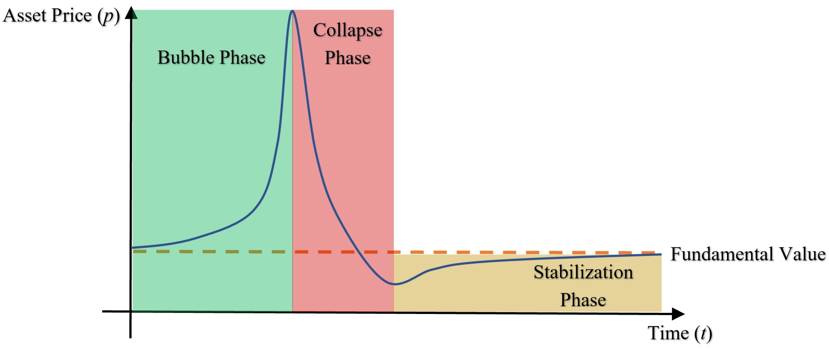
Thus, as mentioned previously, an asset bubble can be taken to comprise three basic stages, namely a
bubble phase, in which irrational exuberance brings about an unsustainable growth in the asset’s price; a
collapse phase, in which investors liquidate their positions and flee the market, leading to a precipitous fall in the asset price below the fundamental value; and a
stabilization phase, in which the price begins to recover and climb slowly back to the fundamental value due to the market demand and supply returning to their prebubble rational equilibria. We illustrate these three phases qualitatively in
Figure 1.
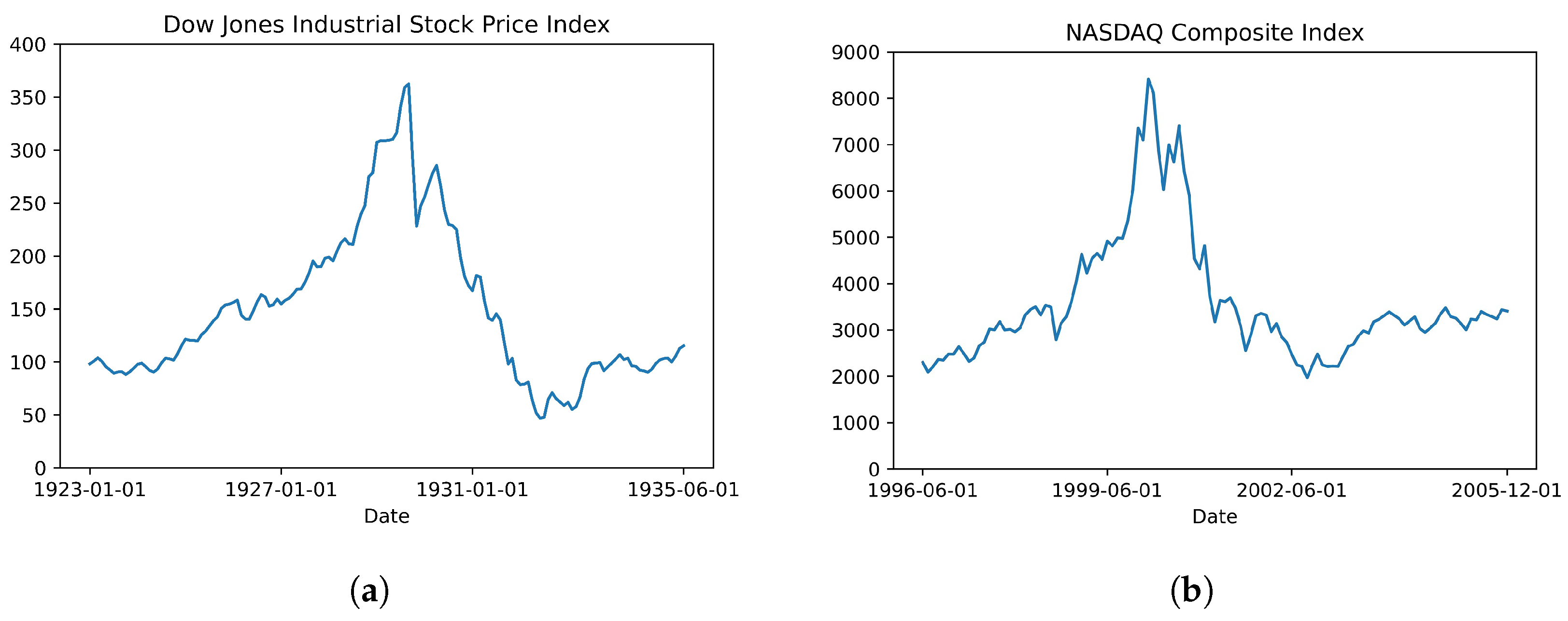
These general price trends (bubble phase, collapse phase, and stabilization phase) can be historically observed in several real-world markets. According to Barlevy [
1], one instance of the unstable-price-increase definition of financial bubbles is the United States stock market over the course of the 1920s. In fact, he references the meteoric rise and subsequently precipitous collapse of the Dow Jones Industrial Average (DJIA) in the late 1920s and early 1930s as a commonly mentioned example of this bubble definition, alongside the seventeenth century’s tulipmania. The price trends of the Dow Jones Industrial Stock Price Index from 1 January 1923 to 1 June 1935 are given in
Figure 2a (source: [
18]). Note that according to the data from the Federal Reserve Bank of St. Louis [
18], the Dow Jones index grew substantially in value until late 1929 (bubble phase), followed by a precipitous fall to a minimum value in 1932 (collapse phase) and a gradual recovery back up toward the fundamental value (stabilization phase).
Another instance of these expected price trends is the NASDAQ Composite Index over the course of the Dot-com Bubble, whose historical values from 1 June 1996 to 1 December 2005 are depicted in
Figure 2b (source: [
19]). Note that the historical NASDAQ Composite Index values from the time of the Dot-com Bubble also display the expected trends of unsustainable growth, abrupt collapse, and moderate upward recovery.
Another important price trend discussed by Kiselev and Ryzhik [
9] is the phenomenon of
serial bubbles, in which bubbles follow one another in succession in the same market. One reason the authors give for the formation of such serial bubbles is that the upward price trends taking place in the recovery phase (as prices rise back toward the fundamental value) may be significant enough to provoke the formation of another bubble in the market [
9].
Hence, the primary objective of this study is to build a behavioral mathematical model that yields price trends consistent with the expected bubble phase, collapse phase, and stabilization phase of financial bubbles as depicted in
Figure 1 and, if possible, also consistent with alternate market trends such as serial bubbles.
3. Building the Behavioral Model
3.1. Model Assumptions
To build a behavioral mathematical model of financial bubbles that incorporates herd behavior and price dynamics, it is necessary to first outline some of the assumptions inherent in the model.
First, similarly to Korobeinikov’s work [
16], the model is assumed to operate in an economy (or community) composed of
C individual agents, where there is no influx of participants.
Second, we assume that the participants in the economy are homogeneous, i.e., all investors have equal purchasing power (purchase equal amounts of the asset at a given price) and influence on their peers (equal degrees of authority, credibility, and publicity such that no participants have `celebrity’ status in the market).
Third, the model assumes that the participants in the economy consist of three groups, namely (i) neutrals, who are neither supportive of nor opposed to investing in a particular asset (and have neither a long position in the asset nor are engaged in selling it but who are still in the market); (ii) optimists, often referred to as `bulls’, who are convinced of the value of investing in the asset (and who are entering or have entered into a long position in the asset in question); and (iii) pessimists, often referred to as `bears’, who are convinced of the need to liquidate their investment in the asset (and who wish to sell their investment and liquidate their long position in the market).
It is also assumed that the pessimists/bears will eventually (and permanently) quit the market altogether (predominantly by selling the asset), thereby converting into a subpopulation of quitters. Notice that the neutral individuals, who are not currently purchasing, holding, or selling the asset, can still be influenced by investor sentiment, unlike the quitters.
Thus, the model assumes that the population in the economy is divided into four groups, namely neutrals, denoted as ; optimists/bulls, denoted as (from the Latin term for bull, taurus); pessimists/bears, denoted as (from the Latin term for bear, ursus); and quitters, denoted as .
Finally, to avoid complications, the process of short selling is ignored in the model (such that purchasing and owning the asset is assumed to be a necessary prerequisite for selling it), and it is assumed that there is no economic growth or inflation in the market over the lifetime of the bubble (such that the fundamental value of the asset is held to be constant indefinitely in both real and nominal terms).
On the basis of these assumptions, we introduce the equations describing the dynamics of an asset price in
Section 3.2, the equations describing the social contagion dynamics of the economy’s population in
Section 3.3, and the full mathematical model of financial bubbles in
Section 3.4.
3.2. Price Dynamics
Based on the assumption of economic equilibrium, where a stable asset price is attained by the balance of supply and demand, the following Evans price equilibrium model [
17,
20,
21,
22], which describes the rate of change of price with respect to time as a function of the difference between demand and supply, is used:
where
, and the demand and supply functions of price are expressed as:
where
and
denote the autonomous demand and price elasticity of demand, respectively, and
and
denote the autonomous supply and price elasticity of supply, respectively.
Since the market demand depicts the quantity of the asset that participants are willing to purchase at a given price and only optimists/bulls () are engaged in purchasing the asset, it is reasonable to think of the market demand as an increasing function of the number of optimists () in the economy. Similarly, since the market supply depicts the quantity of the asset that participants are willing to sell at a given price and only pessimists/bears () are engaged in selling the asset, it is also reasonable to think of the market supply as an increasing function of the number of pessimists () in the economy.
Therefore, we must adapt Equation (
1) in such a way that the demand is a function of the number of optimists/bulls (
) in the economy and the supply is a function of the number of pessimists/bears (
) in the economy.
3.2.1. Demand Function
Let us address the demand function first. As previously mentioned, positive bubbles are characterized by excess demand for an asset [
3], and since only the optimists/bulls (
) are engaged in purchasing the asset, it is reasonable to think that the market demand, as expressed by Equation (
2), should be an increasing function of optimists.
In order to unfold the effect of the number of optimists on the demand, recall that the price elasticity (
) is a parameter that describes the change in the quantity demanded for a given change in price and that the presence or availability of substitutes for an asset results in a greater price elasticity of demand [
23,
24]. Since growing optimism and zeal reduces the asset’s perceived substitutability (potential substitutes are viewed as not obtaining comparable returns), this perceived decline in substitutes must reflect a decrease in the price elasticity of demand.
As such, the price elasticity (
) is appropriately understood as a function of the optimist/bull population (
); the more numerous the optimists/bulls in the market, the more price-inelastic the demand curve will become. A basic rational function describing this situation is:
where the parameter
characterizes the effect of the bull population on the price elasticity of demand, and
(with
) denotes the basal price elasticity of demand.
Now, let us turn our attention to the autonomous demand (
), which is the quantity of the asset demanded when prices equal zero [
17]. Assuming that this quantity increases according to the number of optimists and that the contribution of each optimist/bull in the market toward autonomous demand is the same, the autonomous demand function reflecting its dependence on the optimist population can be written in the following form:
where
characterizes the effect of the bull population on the autonomous demand, and
denotes the stable autonomous demand level in the absence of bulls.
Therefore, the overall demand function used to describe the price dynamics during the formation of a bubble takes the following form:
where
.
3.2.2. Supply Function
Turning now to the supply function in Equation (
2), recall that negative bubbles (and, by extension, collapsing bubbles) are characterized by general market pessimism and excess supply of the asset [
3]. Since pessimistic investors seek to liquidate their investments by selling the asset and thereby contribute to the market supply, it is reasonable to assume that this growing pessimism among investors in the asset serves as the underlying cause of excess supply and that the supply function (
) should be an increasing function of the number of pessimists/bears (
).
Unlike the case of the price elasticity of demand () discussed previously, the price elasticity of supply () is subject to two opposing effects during the collapse phase of the bubble cycle as the number of bears () grows.
The first effect arises from investors who are
risk-averse and thus tend to avoid risk in lieu of improved certainty [
25]; as such, risk-averse investors would prefer to liquidate (sell) their position in the market and eliminate their risk, even if doing so implies a loss on investment. In fact, risk aversion leads investors to prefer to incur a cost rather than face a higher level of risk [
26]. Such pessimistic investors may be assumed to exhibit a decreased interest in the price at which they sell their investment (instead prioritizing liquidating their position at any viable price), which would correspond to a decrease in the price elasticity of supply (
) of the asset.
Meanwhile, the second effect arises from investors who are
loss-averse, who are commonly understood as investors with a steeper utility function (and, hence, a greater dislike) for losses than (their preference) for gains [
27]; this loss aversion is a common form of myopic behavior among investors [
28]. These loss-averse investors would therefore be unwilling to sell the asset at a loss and choose instead to maintain their positions and wait out the fall in price for as long as necessary. Since such loss-averse investors become more hesitant to sell during the fall in asset price, loss-averse behavior results in an increase in the price elasticity of supply (
).
Therefore, the two forces of risk aversion and loss aversion work in opposite directions during the collapse period of the bubble cycle, with the former leading to a decrease in price elasticity of supply and the latter leading to an increase in the same. Because the magnitude of each of these forces in the market is unknown, it is uncertain which behavioral effect (if any) would override the other and lead to an increase or decrease in the overall price elasticity of supply. Therefore, for the sake of simplicity, it is assumed that the price elasticity of supply () is independent of the number of bears () and held at a constant value () (stable price elasticity of supply) throughout the entire bubble cycle, i.e., .
Concerning the autonomous supply, represents the amount supplied when prices equal zero. It is assumed that the underlying asset in the market has some positive intrinsic value; therefore, suppliers or investors will always be unwilling to give it away for free (), and the autonomous supply will be subject to the condition .
However, investors’ willingness to sell the asset at a particular price will vary with the level of pessimism in the market. As the number of pessimists/bears () grows in the market and increasing numbers of investors liquidate their positions, the asset supply increases accordingly, and investors also begin selling the asset at prices that were previously considered too low to sell. This brings about a corresponding increase in the autonomous supply () (equivalent to a decrease in its absolute value). Since the asset is assumed to have positive intrinsic value, the autonomous supply must remain negative and is taken to fulfill as .
Hence, the autonomous supply (
) can be expressed in the following simple rational function form:
where the parameter
characterizes the effect of the bear/pessimist population on the autonomous supply, and
(where
) denotes the stable autonomous supply level in the absence of pessimists.
Combining the functions of the two supply parameters (
and
), the overall supply function used to describe the price dynamics in our model takes the following form:
where
.
Denoting the demand and supply curves in the absence of a bubble (i.e.,
) as
D and
S, respectively, and those in the presence of a bubble as
and
, respectively, the shift in the demand curve (from
D to
) as the number of bulls (
) increases and the shift in the supply curve (from
S to
) as the number of bears (
) increases are depicted qualitatively in
Figure 3.
3.2.3. Overall Price Equation
Now that the supply and demand functions depending on the bull/optimist and bear/pessimist populations have been constructed, we adapt the differential Equation (
1) to a situation in which a bubble is present and obtain the following differential equation describing the price dynamics of an asset in terms of supply and demand functions affected by the presence of bulls (
) and bears (
):
where
and the demand and supply functions are expressed by Equations (
5) and (
7), respectively, whose substitution into Equation (
8) yields:
which, after rearrangement of its right-hand side, becomes the final price differential equation to be used in our financial bubble model.
where
, and
and
denote the pessimist and optimist populations at time
t, respectively.
Before building the equations describing the social contagion dynamics, note from Equation (
10) that the price dynamics in the absence of a bubble (i.e.,
) are described by the following differential equation:
Thus, under the assumption of an economic equilibrium, the stable asset price attained by the balance of supply and demand (ignoring inflation and other potential confounding factors), i.e.,
, is given by
This price level determines the fundamental value of the asset and is taken as the starting price point from which the bubble emerges (i.e., the initial condition for the price), as well as the price level to which the market should converge once the bubble has exhausted itself.
3.3. Behavioral Contagion Dynamics
Now that we have established the dynamics of the price of an asset (
), we need to describe the social contagion dynamics of the full population in the economy during a bubble in terms of the major players in the market, namely bulls/optimists (
) and bears/pessimists (
) (see Equation (
10)), as well as the neutral (
) and quitter (
) groups.
Recall that bubbles form from the introduction of some type of information that appears to promise great future prospects for a particular asset or market [
3]. We assume that prior to this information, the full population in the economy is neutral and of size
C (thus, no bulls, bears, or quitters are present in the market) and that as soon as the information is introduced, a fraction of this neutral population is immediately converted into optimists; this fraction determines the initial condition (
) of the bull/optimist population for the social contagion dynamics. Furthermore, since the new (positive) information does not convert any investors into bears or quitters, the initial condition for the system of differential equations that describes the dynamics of the neutral (
), optimist (
), pessimist (
), and quitter (
) subpopulations of the economy following the introduction of the information is expressed as:
In order to present the equations that describe the social contagion dynamics, we must first outline how the herd behaviors of the optimists and pessimists are spread (analogously to an infectious disease) among the market population.
Since asset bubble price trends are driven by herd behavior [
3] (as investors become convinced to enter or leave the market after exposure to the optimistic/pessimistic views of their peers), the model assumes that the bull subpopulation (
) will infect members of the neutral subpopulation (
) and convert them into optimists/bulls themselves.
Meanwhile, the extreme growth in price during the bubble phase and plummeting prices during the collapse phase cause some optimistic investors to spontaneously become disillusioned with the market, turning into pessimists/bears and liquidating their positions in an effort to exit the market. These pessimistic/bear investors then also influence their peers, converting bulls () into bears ().
Thus, there are two contagion behaviors to be considered in the model: the optimistic behavior spread from the bulls to the neutral population and the pessimistic behavior spread from the bears to the bull population. Note that due to the assumption of no short selling, the bears cannot influence neutral investors, as they have no long positions to liquidate.
Finally, as mentioned in
Section 3.1, the pessimists/bears quit the market permanently after a given period of time (predominantly by selling their asset), thereby joining the quitter subgroup (
).
Incorporating these behaviors into a system of differential equations, the social contagion dynamics of the market population composed of neutrals, bulls, bears, and quitters take the following form:
where
and
represent the contagion rate of optimistic and pessimistic behavior, respectively;
denotes the rate at which optimists/bulls (
) spontaneously convert into pessimists/bears (
) without outside influence (in other words, the spontaneous rate of pessimism in the market); and
denotes the average time a pessimist stays in the bear group (
) before permanently abandoning the market and becoming a quitter (
).
Note that the dynamics of the market population are mainly driven by herd behavior (and are thus independent of the asset price) and that
In other words, the size of the population in the economy remains constant during the duration of the bubble.
3.4. The Full Model
Now, we consolidate the asset price dynamics and the social contagion dynamics expressed by Equations (
10) and (
14), respectively, to construct the full behavioral bubble model:
subject to the initial condition
where
C is the size of the population in the economy;
denotes the proportionality constant of the difference between demand and supply determining the rate of change of the asset price;
characterizes the effect of the bull population on the autonomous demand;
characterizes the effect of the bear/pessimist population on the autonomous supply;
characterizes the effect of the bull population on the price elasticity of demand;
and
denote the stable autonomous demand level in the absence of bulls and the basal price elasticity of demand, respectively;
and
denote the stable autonomous supply level in the absence of pessimists and the constant price elasticity of supply, respectively;
and
represent the contagion rate of optimistic and pessimistic behavior, respectively;
denotes the rate at which optimists/bulls (
) spontaneously convert into pessimists/bears (
) without outside influence (the spontaneous rate of pessimism in the market); and
denotes the average time a pessimist stays in the bear group (
) before permanently abandoning the market and becoming a quitter (
).
In the next section, we carry out a stability analysis of the model, which enables us to determine its long-term behavior; in particular, we conclude that the bubble will eventually exhaust itself and the asset price will return to its fundamental value.
4. Stability Analysis
Note that the dynamics of the social contagion component of the full model (
17) expressed by its last four equations (or equivalently by Equation (
14)) is independent of the dynamics of the asset price expressed by its first equation (or equivalently by Equation (
10)). Thus, in order to carry out the stability analysis, we first find the steady state (
) of Equation (
14).
Letting
, we obtain
which implies that
and, according to Equation (
16), that
where
.
Therefore, the behavioral component of the model expressed by Equation (
14) has a continuum of equilibria, which we prove below is a global attractor.
Since the equations for the
,
, and
subpopulations in Equation (
14) are independent of the equation for
, we can rewrite the social contagion component of the model as
knowing that
.
The following theorem describes the long-term behavior of Equation (
21).
Theorem 1. LetandThen, for every solution () of (21) such that , we have as . Proof. Noting that the
set is a compact, positively invariant set with respect to (
21), we use LaSalle’s Theorem [
29] to demonstrate the result.
Let function
be defined as
Thus, using Equation (
21), we obtain
Notice that for any invariant set (
) in
E, we must have
. If that were not the case, there would exist a point (
) in
for which
. Since
is invariant,
for
(i.e.,
for
), and consequently,
However, using Equation (
21) and assuming the existence of
, we have
which contradicts Equation (
25). Hence, for any invariant set (
) in
E, we must have
, which implies that the largest invariant set in
E is expressed by
Thus, according to LaSalle’s Theorem [
29],
as
. □
Now that Theorem 1 has been established, we present the theorem concerning the asymptotic behavior of the full bubble model (
17).
Theorem 2. LetandThen, for every solution () of (17) such that and we have - (i)
, and
- (ii)
.
Proof. Part (i) is a straightforward consequence of Theorem 1. Note that set
M corresponds to the continuum of equilibria expressed by Equations (
19) and (
20).
For part (ii), notice that since
as
(according to Theorem 1), the equation for asset price (
10) becomes
Therefore,
□
Hence, we have proven that the bubble will exhaust itself, and as a result, the asset price will eventually return to its fundamental value.
As we are interested in the dynamics of the market before the bubble exhausts itself, the next section focuses on a numerical investigation of the possible price dynamics exhibited by the market over the duration of the bubble.
5. Bubble Dynamics and Price Trends
Now that the global stability of the prebubble market equilibrium (
) has been established, we proceed to test the ability of the bubble model (
17) to reproduce the expected bubble, collapse, and stabilization phases of the asset price (see
Figure 1) during a financial bubble. To do so, we carry out numerical simulations of the model (using the Euler approximation method in Python) with different parameter values.
Recall from
Section 3.3 that bubbles form as a result of the introduction of some type of information that creates an expectation of future prospects for a particular asset. Thus, to set up the initial condition for the bubble model (
17), we assume that prior to this information, the price of the asset is at its fundamental value and that the full population in the economy is neutral and of size
C (i.e., no bulls, bears, or quitters at that time). Moreover, we assume that the information is introduced at time
, which causes a fraction of the neutral population to be converted into optimists; this fraction determines the initial condition (
) of the bull/optimist population. Thus, the initial condition for the bubble model (
17) that describes the dynamics of the asset price (
) and the neutral (
), optimist (
), pessimist (
), and quitter (
) subpopulations of the economy upon the introduction of the information is expressed by Equation (
18).
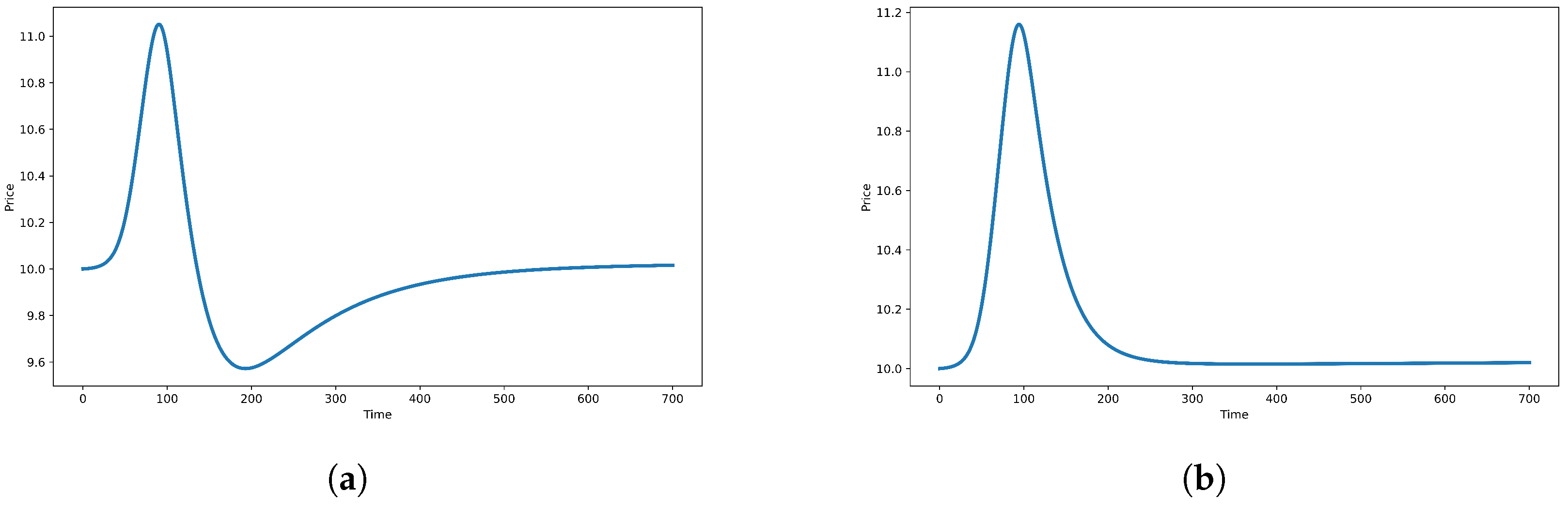
The first numerical simulation for the price dynamics is depicted in
Figure 4a, as obtained by taking the size of the population in the economy (
), initial conditions (
,
,
, and
), and parameter values (
,
,
,
,
,
,
,
,
,
,
, and
). As can be observed, the price trends obtained in
Figure 4a clearly display the bubble phase, collapse phase, and stabilization phase predicted in
Figure 1 (and displayed in the historical price trends of
Figure 2a,b); notably, the asset price falls below the fundamental value during the collapse phase before recovering to the stable (fundamental) value.
Other price dynamics of interest can also be obtained by changing the values of certain parameters. Note that unless otherwise indicated, the value of each parameter is kept the same as in the preceding figure/simulation.
First, a price trend that does not fall below the fundamental value during the collapse phase of the bubble can be obtained by decreasing the parameter value (
to
) (thereby reducing the influence of pessimists/bears on the autonomous supply (
)), yielding
Figure 4b. Note that the collapse phase is not so abrupt as to cause the asset price to fall below its fundamental value, but the price still returns to its fundamental value as
.
Secondly, returning parameter
back to
and decreasing the value of parameter
to
(thereby decreasing the `infectiousness’ of bulls (
)) toward neutral investors (
) yields the trend depicted in
Figure 5a. Although the price dynamics display the bubble, collapse, and upward recovery phases of the bubble cycle, these are followed immediately by another bubble cycle in the market. This is consistent with the phenomenon of serial bubbles as addressed by Kiselev and Ryzhik [
9], who indicate that the recovery phase following a bubble collapse may itself be sufficient to help trigger another bubble.
This phenomenon of serial bubbles is even more evident in
Figure 5b, as obtained by keeping
and increasing the value of
parameter to
(thereby increasing the `infectiousness’ of bears (
)). As can be seen in the figure, the price dynamics exhibit various bubble cycles consisting of the three phases of bubble, collapse, and recovery, in which each bubble is followed immediately by another one (of a progressively smaller amplitude).
Serial bubble behavior is most clearly shown in
Figure 5c, as obtained by increasing the time needed for bears to become quitters to
, increasing the infectiousness of bears to
, and decreasing the value of the
parameter (controlling the impact of bears on the autonomous supply (
)) to
. These modifications slow down the movement of investors into the quitter subgroup, increase the spread of pessimism in the market, and reduce the excess supply during the collapse phase. Note that the three bubble phases of bubble, collapse, and stabilization are clearly displayed in
Figure 5c, as is the serial bubble’s point of transition from stabilizing price trends to the uncontrolled growth of the ensuing bubble.
Finally, another interesting bubble dynamic is depicted in
Figure 5d, as obtained by decreasing the time (
) before a bear becomes a quitter to
. As can be seen in the figure, the price no longer falls to or below the fundamental value during the dynamic fluctuations, instead maintaining a general upward trend in price and losing its oscillatory behavior as prices begin to fall in a more sustained fashion. This occurs because as the time (
) needed for pessimists/bears to convert to quitters decreases, the price collapses over a shorter period of time and hence remains above the fundamental value during the collapse. Although not shown in the figure, the price will return to its fundamental value in the long run.
Overall, the numerical simulations shown in
Figure 5 indicate that serial bubbles are more likely to occur for a lower contagion rate of optimistic behavior (
) and a higher contagion rate of pessimistic behavior (
).
It is worth mentioning that the model can yield a multitude of other price trends (not included in this work) depending on the choice of parameter values describing the social contagion dynamics of the population.
Overall, the numerical outputs obtained in
Figure 4a are consistent with the price trends of bubble, collapse, and stabilization present in the Dow Jones and NASDAQ historical records shown in
Figure 2a,b [
18,
19] and described in
Figure 1. Furthermore,
Figure 5a–c are consistent with the behavior of serial bubbles, in which financial bubbles follow in succession from the previous cycle’s recovery. Hence, the behavioral model developed in this study is capable of exhibiting bubble trends consistent not only with ordinary bubbles but also with serial bubbles as described by Kiselev and Ryzhik [
9].
6. Discussion
The results of this study indicate that observed market price trends can be explained by market behaviors such as social contagion. In particular, the resulting dynamics of the proposed mathematical model confirm our study hypothesis, namely that the bubble, collapse, and stabilization phases of asset bubbles can be explained qualitatively by the processes of investor social contagion. Because we relied exclusively on social contagion to change the market demand and supply, we conclude that the phenomenon of financial bubbles and associated general price trends can be adequately explained from an exclusively behavioral standpoint. The outputs of the model indicate that the fall in prices below the fundamental value before the end of the bubble collapse [
9] can reasonably arise from the behavioral phenomenon of social contagion, as can the appearance of serial bubbles [
9]. As such, the results of this study are consistent with the phenomena associated with financial bubbles outlined by Sornette and Cauwels [
3] and Kiselev and Ryzhik [
9].
This study reinforces the work previously established in the scholarly literature by studying the topic of financial bubbles from a different standpoint. In particular, we used a different underlying methodology than other financial bubble models in the scholarly literature; for instance, unlike other studies that relied on stochastic behavior to construct financial bubble models [
9,
10,
11,
12], we modelled the bubble price trends from a deterministic standpoint. However, unlike the deterministic model constructed by Sornette and Cauwels [
3], which uses the log-periodic power law to depict bubble prices without considering the underlying market dynamics, our model’s price trends are determined by shifts in the market demand and supply curves, which are, in turn, dictated by investor sentiment and social contagion. As such, this study confirms the price trends and underlying behaviors predicted by the scholarly literature [
2,
3,
9].
Furthermore, our investigations reported in
Section 5 demonstrate our model’s versatility in depicting a multitude of possible bubble price trends, indicating that even bubbles that deviate from the three expected phases (bubble, collapse, and stabilization) can be replicated from a herd behavior/social contagion standpoint.
Even though the proposed model properly describes the expected qualitative behaviors of an asset bubble, it also faces certain limitations related to its application to real-world data. For instance, because of the deterministic nature of the model, it is unable to depict the short-term stochastic fluctuations in price that occur in real-world asset markets (an aspect considered in the model developed by Kiselev and Ryzhik [
9]). Also, because of the complexity of market forces and the possibility of spontaneous introduction of information into the market, this model is limited in its ability to predict the timing and, consequently, future course of a bubble (e.g., the timing of collapse or recovery). For example, the model assumes only a one-time introduction of information at the beginning of the bubble cycle but does not account for the near-continuous and stochastic introduction of information that occurs in a real-world market, including random information at different times in the bubble cycle, that could cause the market to fluctuate significantly and deviate from the three expected phases of bubble, collapse, and stabilization. In addition, the model assumes that the market population is constant, when in reality, this population may vary (driven by general population or economic growth or by the introduction of information that either brings more investors into the market or drives them away). This may limit the degree of confidence in a process of model parameter estimation with real-world market data. Even though addressing these limitations in fitting the model to real-world data is beyond the scope of the present study, it can certainly serve as a potential direction for future research.
The particular significance of this work lies not only in the deterministic modelling approach of financial bubbles but, more importantly, in its contribution to explaining and replicating bubble price trends exclusively driven by investor social contagion. As such, this study validates the central role that behavioral phenomena in general and social contagion in particular play in the formation, collapse, and recovery phases of bubbles in asset markets.
However, there remain numerous areas for future investigation and development of the proposed model in order to obtain a more realistic depiction of financial bubbles. For example, further research could be carried out to more accurately ascertain the relationship between investor optimism/pessimism and market demand/supply, which may vary depending on the market; particular attention can be paid to determining how the price elasticity of demand (and supply) are influenced by asset substitutability (and, by extension, investor sentiment). As indicated by Ahern [
24], research on this topic has been generally limited.
Also, as the proposed model focuses on the influence of herd behavior on the dynamics of price, future investigation into how price impacts investor herd behavior could be of great interest. In particular, examination of the changes in the bubble dynamics when one incorporates the effect of price on the spontaneous rate of pessimism () (which was assumed to be a constant parameter in our model), in the proposed model by potentially assuming it to be a function of the asset price could represent a valuable contribution.
It might also be instructive to investigate the effect on the bubble dynamics of an Evans price equilibrium model in which the rate of change of price is described by a nonlinear function of the difference between demand and supply [
21]. Other areas for further investigation and development of this model include studying the effects of a changing market population, a growing fundamental asset value, and inflation on the price trends of the market. The proposed model could also be analyzed in cases in which some (or all) bears/pessimists convert back to neutral status instead of becoming quitters, in a similar fashion to a `leaky vaccine’ in epidemiological modelling [
30,
31,
32]. Finally, it may also be of interest to incorporate a stochastic component into the asset bubble model to yield the short-term price fluctuations of real-world asset prices while keeping the expected (long-term) price trends unchanged.


