Comparative Analysis of the Particle Swarm Optimization and Primal-Dual Interior-Point Algorithms for Transmission System Volt/VAR Optimization in Rectangular Voltage Coordinates

Abstract

Optimal power flow (OPF) is one of the most widely studied problems in the field of operations research, as it applies to the optimal and efficient operation of the electric power system. Both the problem formulation and solution techniques have attracted significant research interest over the decades. A wide range of OPF problems have been formulated to cater for the various operational objectives of the power system and are mainly expressed either in polar or rectangular voltage coordinates. Many different solution techniques falling into the two main categories of classical/deterministic optimization and heuristic/non-deterministic optimization techniques have been explored in the literature. This study considers the Volt/VAR optimization (VVO) variant of the OPF problem formulated in rectangular voltage coordinates, which is something of a departure from the majority of the studies, which tend to use the polar coordinate formulation. The heuristic particle swarm optimization (PSO) and the classical primal-dual interior-point method (PDIPM) are applied to the solution of the VVO problem and a comparative analysis of the relative performance of the two algorithms for this problem is presented. Four case studies based on the 6-bus, IEEE 14-bus, 30-bus, and 118-bus test systems are presented. The comparative performance analysis reveals that the two algorithms have complementary strengths, when evaluated on the basis of the solution quality and computational efficiency. Particularly, the PSO algorithm achieves greater power loss minimization, whereas the PDIPM exhibits greater speed of convergence (and, thus, better computational efficiency) relative to the PSO algorithm, particularly for higher-dimensional problems. An additional distinguishing characteristic of the proposed solution is that it incorporates the Newton–Raphson load flow computation, also formulated in rectangular voltage coordinates, which adds to the efficiency and effectiveness of the presented solution method.

1. Introduction

The electric power supply system serves a critical functionality in modern society. Its primary operational objective is to be able to match the generated power to the load demand at all times. Secure, reliable, economic, and efficient operation of the power system has become one of the pillars of sustainable economic development and social welfare. The primary means used by the system operator to ensure such optimal operation of the power system is referred to as optimal power flow (OPF). OPF developed as an extension of the conventional economic dispatch problem in the early 1960s [1,2]. Over the decades, it has evolved into a variety of network optimization problems employed in all aspects of planning, design, and efficient operation of the entire electric power system. Surveys of OPF formulations and solution techniques have been presented by several authors over the years, for example [3,4,5,6,7]. The focus of the work presented in [3] was on the comparative analysis of the genetic algorithm (GA) and particle swarm optimization (PSO) as they are applied to the OPF problem, with particular attention being paid to the accuracy and computational burden of the two algorithms. The authors of [4] looked at the application of operations research to a number of OPF problems, including expansion planning, unit commitment, and network resiliency. The authors’ main interest was in suggesting how the operations research community could contribute to the advancement of OPF techniques. Reference [5] discussed some of the most recent optimization strategies used to solve OPF problems, falling into the categories of evolutionary, physics-inspired, and human-inspired techniques. The techniques discussed included the GA, evolutionary programming, PSO, differential evolution, the artificial bee colony, the gravitational search algorithm, and the wolf optimization algorithm. The authors of [6] conducted a survey of various classical and heuristic optimization methods that have been applied to OPF over the decades, and presented a critical comparative analysis of the key characteristics of the two classes of optimization methods. Reference [7] presented a review of literature in probabilistic OPF, which seeks to address the stochasticity introduced into electricity networks by variable renewable generation and other distributed energy resources. The main aspects to be considered when it comes to OPF are the problem formulation as well as the solution techniques applied to solve the problem. One of the most practically useful formulations of the OPF problem is the Volt/VAR optimization (VVO) problem, which is mainly concerned with the optimal dispatch of reactive power sources and voltage-regulating devices, and has as the main objective to minimize system losses and enhance the voltage profile of the network. This is important not only for maintaining the security and reliability but also for enhancing the economic operation of the power system [6].

A variety of solution techniques have been applied to the solution of the VVO problem. These fall mainly into the categories of classical/deterministic and heuristic/non-deterministic optimization methods. A bi-level mixed-integer linear programming algorithm has been applied to distribution-level Volt/VAR optimization in [8], with the aim of minimizing voltage deviations. Reference [9] presented a distributed Volt/VAR control algorithm that combines the alternating direction method of multipliers and the column-and-constraint generation algorithm for distribution system power loss reduction and voltage deviation minimization under uncertainty. Heuristic methods have increasingly been attracting more attention among researchers compared with the classical methods. A cooperative particle swarm optimization algorithm (CPSO) has been presented in [10] for Volt/VAR optimization of smart distribution systems. A parallel particle swarm optimization (PSO) algorithm has been proposed in [11] to solve a real-time Volt/VAR optimization algorithm in a large distribution network. Reference [12] combines the PSO and the Non-dominated Sorting Genetic Algorithm II (NSGA-II) to solve a two-stage multi-objective Volt/VAR optimization coordination problem for an electric distribution network. The NSGA algorithm is also applied in [13] for solving the combined optimal active and reactive power dispatch problem. In [14], an adaptive multi-objective Volt/VAR optimization algorithm based on the artificial immune algorithm has been presented, considering active power loss minimization, voltage stability maximization, and voltage level maintenance. Evolutionary algorithms have been applied in [15] to a multi-objective Volt/VAR optimization problem for a distribution network. Reference [16] considers deep reinforcement learning-assisted co-optimization of Volt/VAR services in distribution networks. The authors of [17] applied the biogeography-based optimization (BBO) algorithm to the solution of a multi-objective OPF, including optimal reactive power dispatch. BBO is a biology-inspired, population-based heuristic optimization algorithm in which solutions are treated as habitats and models of biogeography are applied to determine the best available solution. The grey wolf optimizer (GWO) has been applied in [18] to solve the optimal reactive power dispatch problem The GWO algorithm mimics the leadership hierarchy and hunting behavior of grey wolves and tries to apply the concept of group hierarchy to classify the fitness of a solution to an optimization problem.

Among the performance characteristics of optimization algorithms, the ability to find the best available solution (i.e., solution quality) as quickly as possible (i.e., computational efficiency) ranks very highly [19]. For population-based metaheuristic algorithms, such as particle swarm optimization, the genetic algorithm, evolutionary programming, biogeography-based optimization, and grey wolf optimization that have been reviewed above, parameter selection and complexity of algorithm dynamics play a key role in their effectiveness and applicability to different classes of problems. The PSO algorithm has been considered in this study for its desirable properties of having very few parameters to set and being simple to implement, requiring only basic arithmetic operations, and yet able to generate rich dynamic behavior of the collective swarm that proves to be very effective in searching for a solution in the optimization search space [6].

The main focus of this article is to present a comparative analysis of the particle swarm optimization (PSO) algorithm and the primal-dual interior-point method (PDIPM), both applied to the solution of the Volt/VAR optimization problem. A detailed design and implementation of the PSO-based VVO algorithm is presented in this article, whereas the detailed design and implementation of the PDIPM-based VVO algorithm has been presented by the authors in [20]. After presenting the design and implementation of the PSO-VVO algorithm as well as the detailed analysis of four case studies (the same set of case studies considered in [20]), the article then presents the comparative performance analysis of the two algorithms. The Volt/VAR optimization problem is formulated in the rectangular voltage coordinates and incorporates the Newton–Raphson load flow computation, also formulated in rectangular coordinates, as presented in [20]. The reason for the choice of the rectangular coordinate formulation over the polar formulation is the relative computational advantage of the former. For the Volt/VAR optimization problem, the rectangular formulation implies that the objective and constraint functions are quadratic and the Hessian matrices are constant. This is especially advantageous for the PDIPM algorithm, which is solved using the Newton method. Further details are provided in the companion article [20]. The comparative performance analysis of the two algorithms presented in this article reveals key insights into the important performance characteristics of the two approaches to optimization (i.e., heuristic vs. classical approaches) and may serve as a useful aid in the development and design of advanced optimization methods that combine their synergistic properties to devise more efficient algorithm.

The main contributions of this article are outlined as follows:

• Detailed development and implementation of the PSO-based Volt/VAR optimization algorithm, showing how the generic PSO algorithm is adapted for application to the VVO problem formulated in rectangular coordinates;
• Incorporation of the Newton–Raphson load flow computation (also formulated in rectangular coordinates) into the PSO-VVO algorithm, which gives the algorithm the desirable characteristic of being feasible with respect to the active and reactive power flow constraints at every iteration of the PSO-VVO algorithm. The detailed implementation of the Newton–Raphson load flow computation has been presented by the authors in [20];
• A comprehensive comparative performance analysis of the PSO-VVO and the PDIPM-VVO algorithms, making use of four case studies of sizes ranging from the 6-bus to the 118-bus test systems. Each case study has been thoroughly discussed in terms of computational characteristics (i.e., number of iterations needed for convergence and execution time) and solution quality (i.e., power loss minimization and voltage profile improvement achieved);
• An analysis of the impact of the swarm size on the solution quality of the PSO-VVO algorithm.

The rest of the article is organized as follows. Section 2 presents the problem formulation of the Volt/VAR optimization problem. Section 3 provides background information about the PSO algorithm, as well as the design and implementation aspects of the standard PSO algorithm. The application of the PSO algorithm to the solution of the VVO problem is then presented in Section 4. Section 5 presents the simulation case studies, and the comparative analysis of the PSO algorithm with the PDIPM is performed in Section 6. Section 7 concludes the article with a summary of the main results of the study.

2. Formulation of the Volt/VAR Optimization Problem in Rectangular Coordinates

The Volt/VAR optimization problem can be classified as a static constrained nonlinear optimization problem. It is static in the sense that the objective function and decision variables do not vary with respect to time over the duration of the optimization process [21]. And, the optimization is subject to a combination of linear and nonlinear constraints. A mathematical definition of the optimization problem consists in specifying the objectives of optimization, the constraints to be satisfied in the course of the optimization, and the decision or control variables used in the optimization process.

Table 1. Main components of the Volt/VAR optimization problem formulation.

Optimization Problem Component	Key Characteristics	Typical Choices
Objectives of optimization	– Linear/nonlinear; – Convex/nonconvex; – Single-/multi-objective.	– Power loss minimization; – Voltage stability maximization; – Control effort minimization; – Network voltage profile improvement.
Constraints of optimization	– Linear/nonlinear; – Convex/nonconvex.	– Functional (e.g., power flow equations); – Operational (e.g., branch flow limits); – Control variable lower/upper bounds (e.g., generator voltage magnitudes).
Decision/control variables	– Continuous/discrete	– Generator terminal voltages; – Under-load tap-changer positions; – Shunt reactive power sources; – Flexible AC Transmission System devices.

lists the components of the VVO problem formulation, the key characteristics, as well as typical choices of these components.

In this study, the (real) power loss minimization constitutes the objective of optimization. The impact of the Volt/VAR optimization on the voltage profile of the network is also evaluated. Constraints of optimization include the functional and operational constraints, as listed in Table 1. Generator terminal voltages are taken to be the decision variables.

2.1. General Definitions

In this sub-section, a few expressions that facilitate the statement of the VVO problem in the following sub-section are defined. As a complex quantity, voltage $V_k$ at any given bus $k$ can be represented either in rectangular or polar form. Since the problem formulation in this study is based on the rectangular representation of the system voltages, the rectangular form is of particular interest and can be stated as follows:

$$V_k=e_k+j{f}_k, \forall k\in N$$

(1)

where $N$ represents the total number of buses in the system; $e_k$ and $f_k$ are the real and imaginary components of the bus voltage, respectively. In polar form, the magnitude of the voltage and the corresponding phase angle are given by $\left|V_k\right|=\sqrt{e_k^2+f_k^2}$ and ${\tan }^{-1}\left(\raisebox{1ex}{$f_k$}\!\left/ \!\raisebox{-1ex}{$e_k$}\right.\right)$, respectively. The active and reactive power injections at bus $k$ are expressed in rectangular coordinates according to Equations (2) and (3), respectively.

$$P_k=G_{kk}\left(e_k^2+f_k^2\right)+e_k{\displaystyle \sum _{j\in L_k}{G}_{kj}{e}_j-B_{kj}{f}_j}+f_k{\displaystyle \sum _{j\in L_k}{G}_{kj}{f}_j+B_{kj}{e}_j},$$

(2)

$$Q_k=-B_{kk}\left(e_k^2+f_k^2\right)+f_k{\displaystyle \sum _{j\in L_k}{G}_{kj}{e}_j-B_{kj}{f}_j}-e_k{\displaystyle \sum _{j\in L_k}{G}_{kj}{f}_j+B_{kj}{e}_j}$$

(3)

where $L_k$ represents the set of branches directly connected to bus $k$; $G_{kj}$ and $B_{kj}$ represent the real and imaginary components of the kj^th element of the bus admittance matrix (i.e., $Y_{kj}=G_{kj}+j{B}_{kj}$).

The real power transmission losses, which are considered to be the objective function in this study, can be expressed in rectangular coordinates as a summation of the losses in each of the branches of the network, according to Equation (4) [22]:

$$P_{Loss}={\displaystyle \sum _{(k,j)\in L}{G}_{kj}\left[{\left(e_k-e_j\right)}^2+{\left(f_k-f_j\right)}^2\right]}.$$

(4)

2.2. Statement of the Volt/VAR Optimization Problem

Making use of the definitions presented in the preceding sub-section, the statement of the Volt/VAR optimization problem formulated in rectangular coordinates can be expressed as [20]

$$\min P_{Loss}\left(e,f\right)$$

(5)

subject to

$$P_k\left(e,f\right)+P_{dk}-P_{gk}=0,$$

(6)

$$Q_k\left(e,f\right)+Q_{dk}-q_k-Q_{gk}=0,$$

(7)

$$Y_{kj}^2\left[{\left(e_k-e_j\right)}^2+{\left(f_k-f_j\right)}^2\right]\le {\left(I_{kj}^{\max }\right)}^2 ,$$

(8)

$${\left(V_k^{\min }\right)}^2\le e_k^2+f_k^2\le {\left(V_k^{\max }\right)}^2,$$

(9)

$$Q_{gk}^{\min }\le Q_{gk}\le Q_{gk}^{\max },$$

(10)

$$q_k^{\min }\le q_k\le q_k^{\max }.$$

(11)

In the above formulation, $P_{gk}/P_{dk}$ and $Q_{gk}/Q_{dk}$ represent the active and reactive power generation/demand at bus $k$, respectively, $I_{kj}$ denotes the branch current magnitude in branch $kj$, $q_k$ represents the shunt reactive power compensation at bus $k$, and $V_k$ denotes the magnitude of the bus voltage at bus $k$. The objective function is represented by Equation (5); Equations (6) and (7) constitute the active and reactive power flow balance equations; branch flow limits are expressed by Equation (8); and Equations (9)–(11) constitute the boundary constraints on the bus voltages, generator reactive power outputs, and shunt reactive power injections at the buses, respectively. The following section introduces the particle swarm optimization (PSO) algorithm, which has been applied to the solution of the Volt/VAR optimization problem in this study.

3. Particle Swarm Optimization (PSO) Algorithm

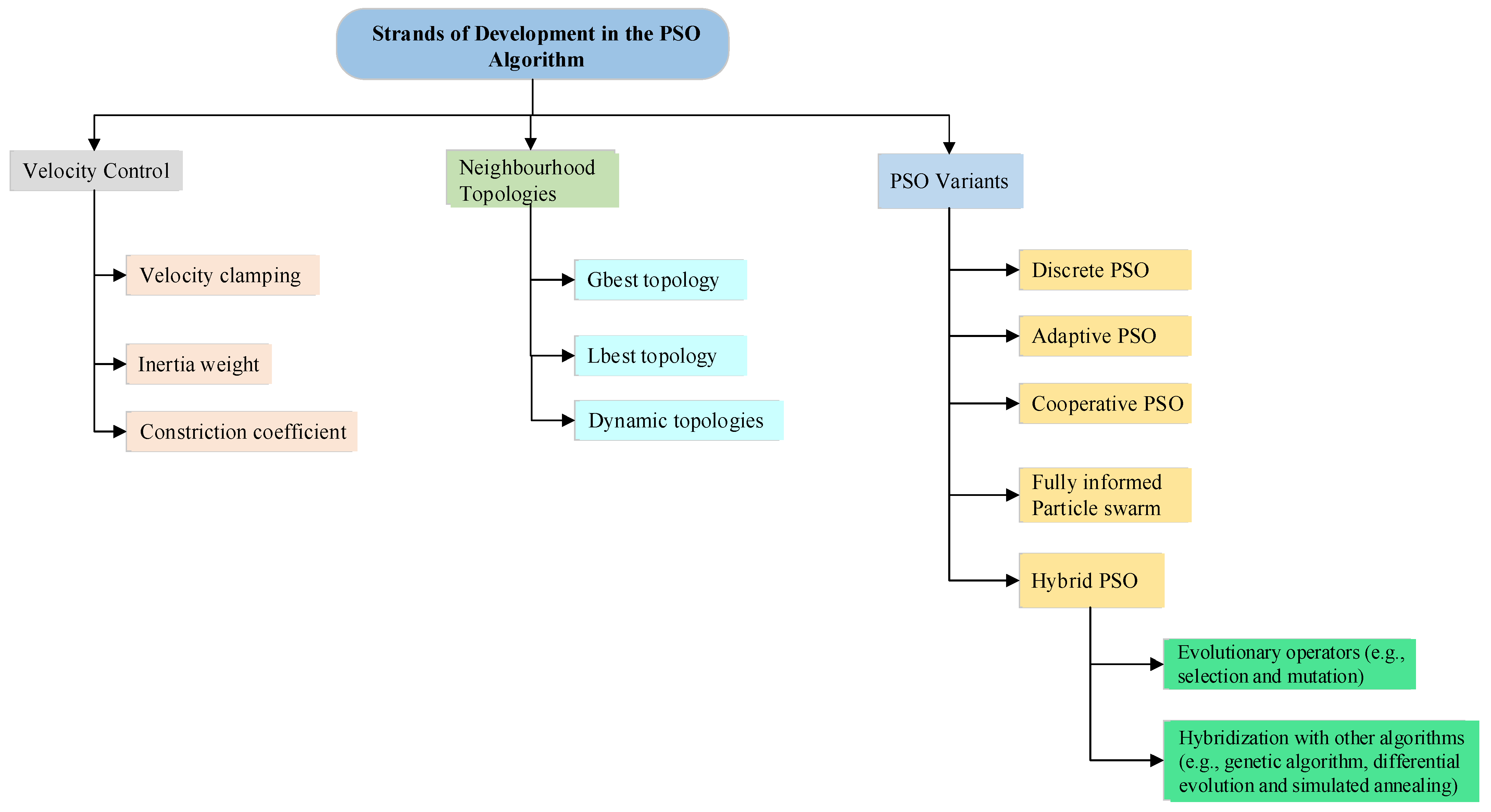
3.1. Historical Development of the PSO Algorithm

Particle swarm optimization (PSO) belongs to the class of heuristic optimization techniques collectively referred to as Swarm Intelligence, which constitutes a stream of Artificial Intelligence (AI) research that was established in the early 1990s; it is based on the study of the swarm behavior of natural creatures, in terms of how the decision making of the individual is influenced by both the individual’s own experience and the experiences of community members. PSO was conceptualized and developed by J. Kennedy, a social psychologist, and R. Eberhart, an Electrical Engineer [23]. The main idea behind their conceptualization was to produce computational intelligence by exploiting simple analogues of social interaction among conspeciates and was inspired by the works of Reynolds [24] and Heppner and Grenander [25]. Reynolds, as well as Heppner and Grenander, had studied the dynamics of bird social behavior, out of which came the conjecture that the aesthetics and synchrony of flocking behavior exhibited by birds was a function of the birds’ efforts to maintain an optimal inter-individual distance among neighboring members of the flock.

A distinctive feature of PSO is the idea of flying candidate solutions through hyperspace in search of better solutions. The algorithm is characterized by simplicity and robustness. Its implementation requires only a few lines of code, making use of only primitive mathematical operators with modest memory requirements and only few parameters that need to be specified for any given problem. Out of this “natural simplicity” that is based on emulating nature emerges a powerful algorithm that has proved to be effective for a wide range of applications, notably the training of artificial neural network weights [26].

Since its conceptualization in the early 1990s and eventual implementation in the subsequent years, the PSO has undergone a number of developments:

• The introduction of new parameters (e.g., inertia weight and constriction factor) to improve the algorithm’s convergence characteristics;
• Modification of the basic algorithm to tailor it to different problem types (e.g., cooperative PSO);
• Hybridization with other heuristic optimization techniques to enhance the effectiveness and efficiency of the algorithm.

Figure 1 provides a summary of these notable developments. Some of them are further discussed in subsequent sections in this article.

3.2. Principle of Operation and Basic Formulation of the PSO Algorithm

PSO can be characterized as a stochastic multi-agent parallel search algorithm in which each of a swarm of particles represents a candidate solution to an optimization problem. A particle can be thought of as an independent intelligent agent that “flies” through a multi-dimensional problem space in search of the optimal solution to the optimization problem, based on its own past flying experience and that of the rest of the swarm [26]. Each particle $i$ in the swarm is comprises three n-dimensional vectors (n being the dimensionality of the search space, $R^n$), which at time $k$ can be denoted as the current position, $X_i^k$, the previous best position, $P_{best,i}^k$, and the velocity, $V_i^k$ [27].

The current position of each particle, $X_i^k$, constitutes the decision vector, which at each iteration is evaluated for “fitness” by means of the objective function of the optimization problem. The particle velocity, $V_i^k$, embodies the composite flying experience of the individual particle and of the rest of the swarm and is used to update the individual particle position in an effort to advance it to a “better” position, as judged by it attaining an improved fitness evaluation. Each particle keeps track of the position corresponding to the best fitness value it has attained up to the latest iteration, denoted as $P_{best,i}^k$, which is then updated to the current position whenever the current position results in a better fitness value than the previous best value. As the iterations progress, the swarm as a whole, much like a flock of birds foraging for food, is likely to move towards the optimal point in the search space. The social interaction and information sharing among the swarm’s particles is a very important characteristic of the PSO algorithm. It is the collective behavior of the swarm that gives the algorithm its optimum searching capability [23].

The core component of the PSO algorithm is the iterative velocity update, which adjusts each particle’s position so as to drive the entire swarm towards the optimal solution to the optimization problem. The standard algorithm is presented in the flowchart in Figure 2 [27].

$$\{\begin{array}{l}{\overrightarrow{V}}_i^{k+1}={\overrightarrow{V}}_i^k+\overrightarrow{U}\left(0,{\phi }_1\right)\otimes \left({\overrightarrow{P}}_{best,i}^k-{\overrightarrow{X}}_i^k\right)+\overrightarrow{U}\left(0,{\phi }_2\right)\otimes \left({\overrightarrow{G}}_{best}^k-{\overrightarrow{X}}_i^k\right)\\ {\overrightarrow{X}}_i^{k+1}={\overrightarrow{X}}_i^k+{\overrightarrow{V}}_i^{k+1}\end{array}$$

(12)

In Equation (12), $\overrightarrow{U}\left(0,{\phi }_1\right)$ represents a vector of random numbers uniformly distributed in $\left[0, {\phi }_1\right]$ generated for each particle at each iteration. The symbol $\otimes$ denotes component-wise multiplication. The parameters ${\phi }_1$ and ${\phi }_2$ are commonly referred to as acceleration coefficients. Their magnitudes determine the relative influence of the cognitive and social components on the flight of the particle.

A distinctive feature of the standard PSO algorithm (particularly when compared with other heuristic optimization techniques) is that it has relatively few parameters that need to be set for a given problem. The main PSO parameters are outlined and briefly discussed in

Table 2. Key parameters of the PSO algorithm.

Parameter Type	Description
Swarm size	Number of particles or population size of the particle swarm; A large swarm size leads to a wider search space (desirable) but also implies a higher computational cost (drawback); Swarm size in the range (20-60) has been found to suffice for many applications [27,28].
Number of iterations of the algorithm	A sufficiently large number improves the likelihood of finding the best available solution; Too large a number may lead to a prohibitive computational cost; The type of problem may impact the decision regarding the suitable maximum number of iterations.
Velocity update	Comprises three components: the inertial (${\overrightarrow{V}}_i^k$), cognitive ($\overrightarrow{U}\left(0,{\phi }_1\right)\otimes \left({\overrightarrow{P}}_{best,i}^k-{\overrightarrow{X}}_i^k\right)$), and social ($\overrightarrow{U}\left(0,{\phi }_2\right)\otimes \left({\overrightarrow{G}}_{best}^k-{\overrightarrow{X}}_i^k\right)$) components; The relative values of the acceleration constants determine the contribution of each component to the overall velocity update; A good balance between the cognitive and social components has been found to work well for many problem types [28].

.

3.3. Implementation Aspects of the PSO Algorithm

The algorithm presented in the previous section requires a few enhancements and additional considerations in order to improve its efficiency and effectiveness for practical implementation purposes. Particularly, the following implementation aspects are briefly discussed in this section, as further detailed in

Table 3. Important implementation aspects of the PSO algorithm.

Implementation Aspect	Considerations and Guidelines
Exploration/exploitation trade-off balance	Exploration promotes coverage of as wide a search space as possible in the initial phase, whereas exploitation favors concentrated search in a narrower search space in the latter phase of the algorithm execution; Velocity control has a significant impact on achieving the right exploration/exploitation balance.
Velocity control by velocity clamping	Important to keep velocity from building up uncontrollably, Impacts the algorithm’s speed of convergence, and affects the exploration/exploitation balance; Velocity clamping places bounds on the magnitude of ${\overrightarrow{V}}_i^k$ to lie within the range $\left[-V_{\max },+V_{\max }\right]$; Has the drawback that the choice of $V_{\max }$ tends to be problem-dependent and generally has poor velocity control characteristics [29];
Velocity control by inertia weight	Provides an alternative way of regulating velocity update [30]; Applies a scaling to the inertial component of the velocity update in Equation (12) leading to Equation (13); $\omega$ Is referred to as the inertia weight, typically set according to Equation (14), where ${\omega }_{\max }, {\omega }_{\min }$ are the initial and final values of $\omega$, respectively, and $k, k_{\max }$ are the current and maximum iteration number, respectively; Typical values for ${\omega }_{\max }, {\omega }_{\min }$ are 0.9 and 0.4, respectively.
Velocity control by constriction coefficient	Another alternative way of regulating velocity update; Applies a scaling to the entire velocity update formula given by Equation (12) leading to Equation (15), with the constriction coefficient, $\chi$, being set according to Equation (16); Acceleration constants are usually set to be equal, that is, ${\phi }_1={\phi }_2$, with a value just above 2 typical [31].
Initialization of PSO algorithm parameters	As a population-based algorithm, proper initialization of PSO parameters is important for its effectiveness and efficiency; Besides setting values of swarm size, acceleration constants and maximum number of iterations, initial particle positions, and velocities also have to be initialized; Ensuring diversity of initial population is achieved by a randomization operation according to Equation (17), where $X_{\min ,i}$ and $X_{\max ,i}$ are the lower and upper bounds of the magnitude $X_i$, and $r_i$ is a uniformly distributed random number between 0 and 1.
Termination conditions for the algorithm	As an iterative algorithm, termination conditions need to be set for PSO for it to terminate, whether successfully (with the best available solution found) or unsuccessfully. Termination conditions may include: Lack of appreciable (improving) change in the fitness value of the global best position over a number of iterations; Insignificant change in global best position over a number of iterations; Exceeding the predetermined maximum number of iterations. The first and third conditions listed above have been considered in this study.

:

• Balancing the exploration/exploitation trade-off.
• Controlling the velocity to improve convergence characteristics by means of:

  ○

  Velocity clamping;

  ○

  Inertia weight;

  ○

  Constriction coefficient.

• Initialization of algorithm parameters.
• Termination conditions for the algorithm.

$${\overrightarrow{V}}_i^{k+1}=\omega {\overrightarrow{V}}_i^k+\overrightarrow{U}\left(0,{\phi }_1\right)\otimes \left({\overrightarrow{P}}_{best,i}^k-{\overrightarrow{X}}_i^k\right)+\overrightarrow{U}\left(0,{\phi }_2\right)\otimes \left(G_{best}^k-{\overrightarrow{X}}_i^k\right) ,$$

(13)

$${\omega }^{k+1}={\omega }_{\max }-\left(\frac{{\omega }_{\max }-{\omega }_{\min }}{k_{\max }}\right) k , {\omega }_{\max }>{\omega }_{\min },$$

(14)

$$\{\begin{array}{l}{\overrightarrow{V}}_i^{k+1}=\chi \left({\overrightarrow{V}}_i^k+\overrightarrow{U}\left(0,{\phi }_1\right)\otimes \left({\overrightarrow{P}}_{best,i}^k-{\overrightarrow{X}}_i^k\right)+\overrightarrow{U}\left(0,{\phi }_2\right)\otimes \left({\overrightarrow{G}}_{best}^k-{\overrightarrow{X}}_i^k\right)\right)\\ {\overrightarrow{X}}_i^{k+1}={\overrightarrow{X}}_i^k+{\overrightarrow{V}}_i^{k+1}\end{array} ,$$

(15)

$$\chi =\frac{2}{\phi -2+\sqrt{{\phi }^2-4\phi }} , where \phi ={\phi }_1+{\phi }_2>4,$$

(16)

$$X_i^0=X_{\min ,i}+r_i\left(X_{\max ,i}-X_{\min ,i}\right), r_i\in U\left(0, 1\right).$$

(17)

The following section focuses on the adaptation of the PSO algorithm to the requirements of the Volt/VAR optimization algorithm.

4. PSO Algorithm Applied to the Volt/VAR Optimization Problem

The Volt/VAR optimization (VVO) problem formulation has been presented in Section 2. In this section, the PSO algorithm presented in Section 3 is adapted for application to the VVO problem. In applying the PSO algorithm to any optimization problem, the mechanics of the algorithm have to be mapped to the structure of the optimization problem. Particularly, the mapping needs to be made between the particle positions and velocities, and the decision vector of the optimization problem, along with the adjustment process of the decision vector in the search for the optimal solution to the problem. For the VVO problem, the mapping can be stated as follows:

• The decision vector comprises the generator voltages, expressed in rectangular coordinates; thus, each particle is constructed by combining the real and imaginary components of all the generator voltages in the system.
• For the slack bus, the phase angle is required to be maintained at a predetermined constant value, and so the imaginary component of the slack-bus voltage does not form part of the decision vector.
• The length (i.e., number of elements) of each particle is, thus, $2n_g-1$, where $n_g$ represents the number of generators in the system, including the slack-bus generator.
• The velocities of the particles represent the step size adjustments to the decision-vector components (i.e., particle positions), and their computation is one of the main tasks performed in each iteration of the algorithm.

The steps of the PSO algorithm applied to the VVO problem can be outlined as follows.

Step 1:

Load the system parameters: this includes the bus voltages in rectangular coordinates (1), the generator scheduled active generation outputs (reactive generation outputs are set to zero, since they are unscheduled) (2), the load active and reactive power demands (3), and the line impedance (i.e., resistance and reactance) data (3). The impedance and bus connectivity matrices are computed on the basis of the input line data.

Step 2:

Initialize the PSO algorithm parameters: this includes the acceleration coefficients (${\phi }_1, {\phi }_2$), the swarm size, the problem dimension (i.e., number of elements comprising each particle), and the maximum number of iterations.

Step 3:

Compute the initial particle positions and velocities: the particle positions are initialized according to Equation (17), which is reformulated below as it applies to the VVO problem:

$$V_{gen\_i}^0=V_{gen\_i}^{\min }+r_i\left(V_{gen\_i}^{\max }-V_{gen\_i}^{\min }\right), r_i\in U\left(0, 1\right)$$

(18)

where $V_{gen\_i}^0$ is the ith generator’s initial voltage magnitude and $V_{gen\_i}^{\min }, V_{gen\_i}^{\max }$ are the minimum and maximum generator voltage magnitudes, respectively. For the VVO problem, the generator-bus voltage magnitudes have the bounds

$$0.95\le V_{gen}\le 1.1.$$

(19)

So, based on Equation (19), the initial generator voltage magnitude (which corresponds to particle position $X_i$ in Equation (17) can be set according to Equation (18) as

$$V_{gen\_i}^0=0.95+0.15r_i.$$

(20)

In effect, for the rectangular-coordinate representation of the generator voltages, Equation (20) is actually used to compute the real component of the voltage ($e_i$), after which the imaginary component ($f_i$) is computed by means of Equation (21).

$$V_i^2=e_i^2+f_i^2$$

(21)

Initialization of the particle positions by means of Equations (20) and (21) ensures that they are all feasible with respect to the bound constraints according to equation (19).

The initial velocities are set to zero for this study.

Step 4:

Compute each particle’s fitness value based on initial positions: the objective function for the VVO problem in rectangular coordinates is given by Equation (4), which is the transmission real power loss function, restated below for ease of reference:

$$P_{Loss}={\displaystyle \sum _{(k,j)\in L}{G}_{kj}\left[{\left(e_k-e_j\right)}^2+{\left(f_k-f_j\right)}^2\right]}.$$

(22)

The constraints considered in this study are all bound constraints (Equations (8)–(11)). Each bound constraint is handled such that when it violates its bound constraint its value is set to the violated (lower or upper) bound. The generator voltage magnitude, for example, has its value set according to

$$V_{gen\_i}=\{\begin{array}{l}{V}_{gen\_i}^{\min } if V_{gen\_i}<V_{gen\_i}^{\min }\\ V_{gen\_i} if V_{gen\_i}^{\min }\le V_{gen\_i}\le V_{gen\_i}^{\max }\\ V_{gen\_i}^{\max } if V_{gen\_i}>V_{gen\_i}^{\max }\end{array}.$$

(23)

Before computing the fitness values using Equation (22), limit violations are checked and corrected according to Equation (23).

After this initial computation of fitness values, the (initial) personal best position and corresponding fitness value of each particle is set to the current (i.e., initial) position and its corresponding fitness value. That is, for each particle $X_i$,

$$P_{best,i}^0=X_i^0.$$

(24)

The initial global best position is determined as the value of $P_{best,i}^0$ giving the best (i.e., minimum) fitness value, determined as

$$g_{best}^0=\arg \min \left(f\left(p_{best,i}^0\right)\right), i=\overline{1,\dots ,p}$$

(25)

where p is the number of particles in the swarm and the operator $\arg \min ()$ returns the argument $P_{best,i}^0$ that yields the minimum value of the fitness function $f\left(P_{best,i}^{}0\right)$.

Step 5:

Compute the Newton–Raphson load flow: the effect of the PSO algorithm is to adjust the generator voltage magnitude set-points at each iteration of the algorithm. In the proposed PSO-VVO algorithm, a load flow computation is run at each iteration of the PSO algorithm in order to determine the load-bus voltages, subject to the active and reactive power balance equations (Equations (6) and (7), Section 2.2) (please refer to the work of the authors in [20] for a more detailed treatment of the incorporation of the Newton–Raphson load flow computation in the VVO algorithm). For the load flow computation, the global best position ($g_{best}$) is used, since this is assumed to be the best available solution.

Step 6:

Recompute the objective function value: a converged load flow computation implies that the solution obtained in step 4 is feasible with respect to both the equality and inequality constraints of the VVO problem. Recomputing the objective function value following the load flow computation is meant to track the objective value of the current best feasible solution of the optimization problem.

Step 7:

Compute the velocity update and adjust the particle positions: this is essentially the beginning of the iterative loop of the PSO algorithm, where the particle velocity is iteratively computed and then used to adjust the particle position. In this study, the velocity and position update are computed on the basis of Equations (15) and (16), restated below for ease of reference:

$$\{\begin{array}{l}{\overrightarrow{V}}_i^{k+1}=\chi \left({\overrightarrow{V}}_i^k+\overrightarrow{U}\left(0,{\phi }_1\right)\otimes \left({\overrightarrow{P}}_{best,i}^k-{\overrightarrow{X}}_i^k\right)+\overrightarrow{U}\left(0,{\phi }_2\right)\otimes \left({\overrightarrow{G}}_{best}^k-{\overrightarrow{X}}_i^k\right)\right)\\ {\overrightarrow{X}}_i^{k+1}={\overrightarrow{X}}_i^k+{\overrightarrow{V}}_i^{k+1}\end{array},$$

(26)

$$\chi =\frac{2}{\phi -2+\sqrt{{\phi }^2-4\phi }} , where \phi ={\phi }_1+{\phi }_2>4.$$

(27)

That is, the constriction coefficient is used as the velocity regulation mechanism, as outlined in Table 3 in Section 3.3.

Step 8:

Compute the fitness value of each particle and update the personal and global best positions: after adjusting the particle positions, limit violations are checked and corrected for using Equation (23), after which the fitness value of each particle is computed using Equation (22). Once the fitness value of each particle has been computed, the personal best $P_{best,i}^k$ of each particle $i$ is updated as follows:

$$P_{best,i}^k=\{\begin{array}{l}{X}_i^k if f\left(X_i^k\right)<f\left(X_i^{k-1}\right)\\ P_{best,i}^{k-1} if f\left(X_i^k\right)\ge f\left(X_i^{k-1}\right)\end{array}.$$

(28)

Then, the global best position is updated according to Equation (25), restated here for ease of reference:

$$g_{best}^k=\arg \min \left(f\left(p_{best,i}^k\right)\right), i=\overline{1,\dots ,p}.$$

(29)

Step 9:

Recompute the Newton–Raphson load flow: similar to step 5, perform a load flow computation to determine the new load-bus voltages, with the global best position (computed in step 8) acting as the new generator voltage set-points.

Step 10:

Recompute the objective function value: similar to step 6, the objective function value is recomputed to account for the change in the load-bus voltages due to the load flow computation. The recomputed objective function value constitutes the optimal value of the current best feasible solution. The algorithm is assumed to have advanced in the desired direction if the recomputed objective function value is better (i.e., less) than the one computed in the previous iteration.

Step 11:

Check for convergence of the algorithm: the PSO algorithm is considered to have converged successfully to an optimal solution when there is not an appreciable change in the objective function value over a number of successive iterations, and the current objective function value is better than the initial value. Otherwise, it is terminated with a result of “failure” when it fails to achieve an objective function value minimization within the predetermined number of iterations. In summary, the PSO algorithm will be terminated if any one of the following two conditions is satisfied:

• There is no appreciable improvement in the objective function value over a number of successive iterations and the current objective function value is better than the initial one;
• The maximum number of iterations has been reached.

If neither of the two conditions is satisfied, the iteration counter (k) is incremented and the algorithm loops back to step 7, repeating steps 7 to 11 until termination conditions are satisfied. The flowchart in Figure 3 summarizes the steps of the PSO algorithm outlined above as adapted for application to the VVO problem.

5. Case Study Results and Discussion

5.1. Description of the Case Studies

The designed PSO-VVO algorithm is analyzed with the aid of four cases studies based on the 6-bus, IEEE 14-bus, 30-bus, and 118-bus test systems. The case studies were selected with the goal of realizing diversity in system size and test network characteristics, which would facilitate the performance evaluation of the designed algorithm, with particular attention paid to the following performance characteristics:

• Magnitude of loss minimization achieved;
• Degree of voltage profile improvement achieved due to the Volt/VAR optimization;
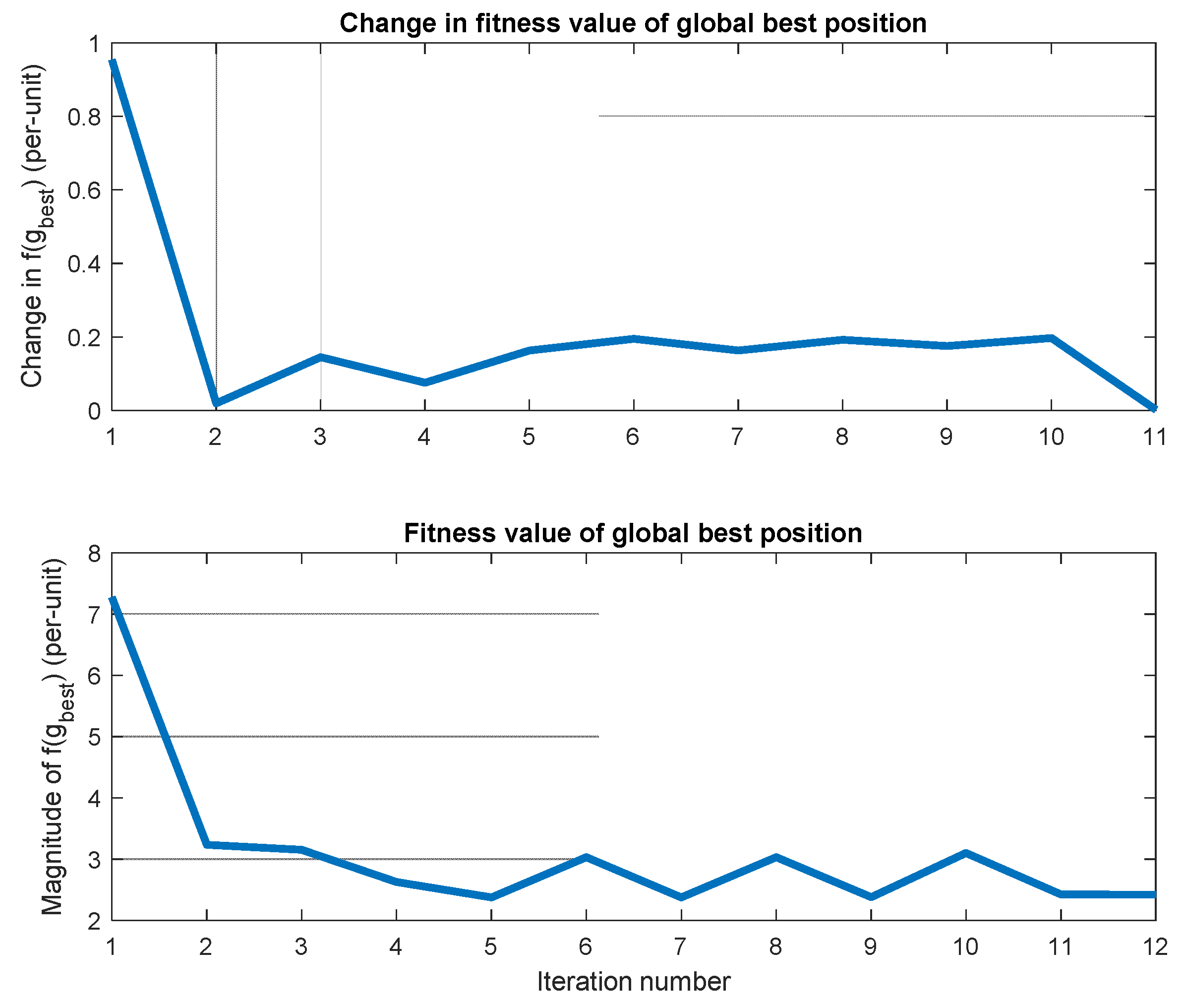
• Efficiency and speed of convergence of the designed algorithm;
• Impact of particle swarm size on the quality of the solution and on the computational efficiency of the algorithm.

The algorithm has been implemented in MATLAB R2023a by MathWorks Inc. [32]. A computer running the Intel(R) Core i7-7700HQ COPU, 2.80GHz, 8 GB RAM, has been used to implement the algorithm and perform the simulation case studies. Data for the 6-bus system has been obtained from [33]. Data for the IEEE 14-bus and 30-bus test systems have been obtained from [34] and the IEEE 118-bus system has been obtained from [35]. The PSO parameters used in the case studies are given in

Table 4. PSO algorithm parameters used in the VVO case studies.

Parameter	Setting
Cognitive acceleration constant, ${\phi }_1$	2.05
Social acceleration constant, ${\phi }_2$	2.05
Swarm size, $p$	10–50
Maximum number of iterations, $k^{\max }$	200

. It can be noted that the swarm size has been specified as a range of values. For each case study, the case is run for values of the swarm size ranging from 10 to 50, in increments of 10. Since PSO is a stochastic algorithm, the approach taken is to make several runs of the algorithm for each value of the swarm size. The statistical variance can then be assessed by looking at the minimum, maximum, and average values of the key results, which can provide insightful information regarding the possible impact of the swarm size on the performance of the algorithm. For each swarm size, 10 independent runs of the algorithm are made, and then averaged. The averaged data is then tabulated for each case study.

5.2. Analysis and Discussion of the Case Study Results

5.2.1. Case Study 1: 6-Bus Power System

This case study is based on a 6-bus power system adapted from [33], which has three generators, eleven lines, and three loads. The performance analysis considers the magnitude of power loss reduction, the degree of voltage profile improvement, the computational efficiency (in terms of the required number of iterations and the corresponding execution time) of the algorithm, and the impact of the particle swarm size, as outlined in Section 5.1. The results of running the PSO algorithm to solve the VVO problem for different swarm sizes are presented in

Table 5. Summary of results of the PSO-VVO algorithm applied to the 6-bus power system.

Swarm Size	Initial Loss (p.u.)			Final Loss (p.u.)			Number of Iterations			Run Time (s)			Average % Loss Reduction
	Min	Max	Average	Min	Max	Average	Min	Max	Average	Min	Max	Average
10	0.1276	0.2441	0.1647	0.1259	0.1339	0.1302	28	71	40	0.0378	0.3638	0.1385	20.95
20	0.1378	0.2885	0.2215	0.1265	0.1318	0.1293	13	102	54	0.0280	0.2056	0.1060	41.62
30	0.1273	0.3275	0.1811	0.1262	0.1336	0.1284	16	56	31	0.0381	0.1363	0.0713	29.10
40	0.1275	0.1670	0.1613	0.1255	0.1302	0.1284	8	32	19	0.0249	0.1531	0.0615	20.40
50	0.1303	0.2212	0.1569	0.1263	0.1332	0.1294	10	133	49	0.0275	0.3185	0.1216	17.53

and in Figure 4, Figure 5, Figure 6 and Figure 7.

The results in Table 5 reveal a consistent and substantial real power loss reduction by the PSO algorithm, with the lowest (average) percentage loss reduction being 17.53% and the highest being 41.62%. The average number of iterations lies in the range between 19 and 54 for all cases. There is quite a large dispersion between the minimum (8) and maximum (133) number of iterations. The execution time shows a similar dispersion (minimum value of 0.0713 s and maximum value of 0.1385 s). Increasing the swarm size does not seem to significantly influence the solution quality. The impact on the computational cost of the algorithm is also not very noticeable.

The convergence behavior of the PSO algorithm applied to the 6-bus system is depicted in Figure 4, which plots the change in the global best position, the change in the fitness value of the global best position, and the fitness value of the global best position in the top, middle, and bottom traces, respectively. This case takes relatively long to converge, about 27 iterations, requiring about 0.04 s. This result can be considered to lie in the middle of the range of the average results presented in Table 5.

The voltage profile of the 6-bus system before and after the Volt/VAR optimization is depicted in Figure 5 in the form of a bar chart. The post-optimization voltage magnitudes are greater than the pre-optimization values for all buses, except bus 2 where the pre-optimization voltage is slightly higher than the post-optimization voltage. In all cases, both the pre- and post-optimization voltages are within the range of nominal values (i.e., 0.95–1.1).

Figure 6 depicts the real power loss trajectory plotted together with the slack-bus active power output against the number of iterations. The plots reveal that reduction in system power loss results in a corresponding reduction in the slack-bus generated power. Indeed, the main reason for having a slack bus in the power system is to compensate for generation-demand imbalances that cannot be known in advance, which includes system losses [36]. A similar relationship can be seen in Figure 7 which plots the real power loss reduction together with the total system reactive power generation, also showing that a reduction in the system real power loss is accompanied by a reduction in the system reactive power generation as well, which further improves the efficiency of system operation.

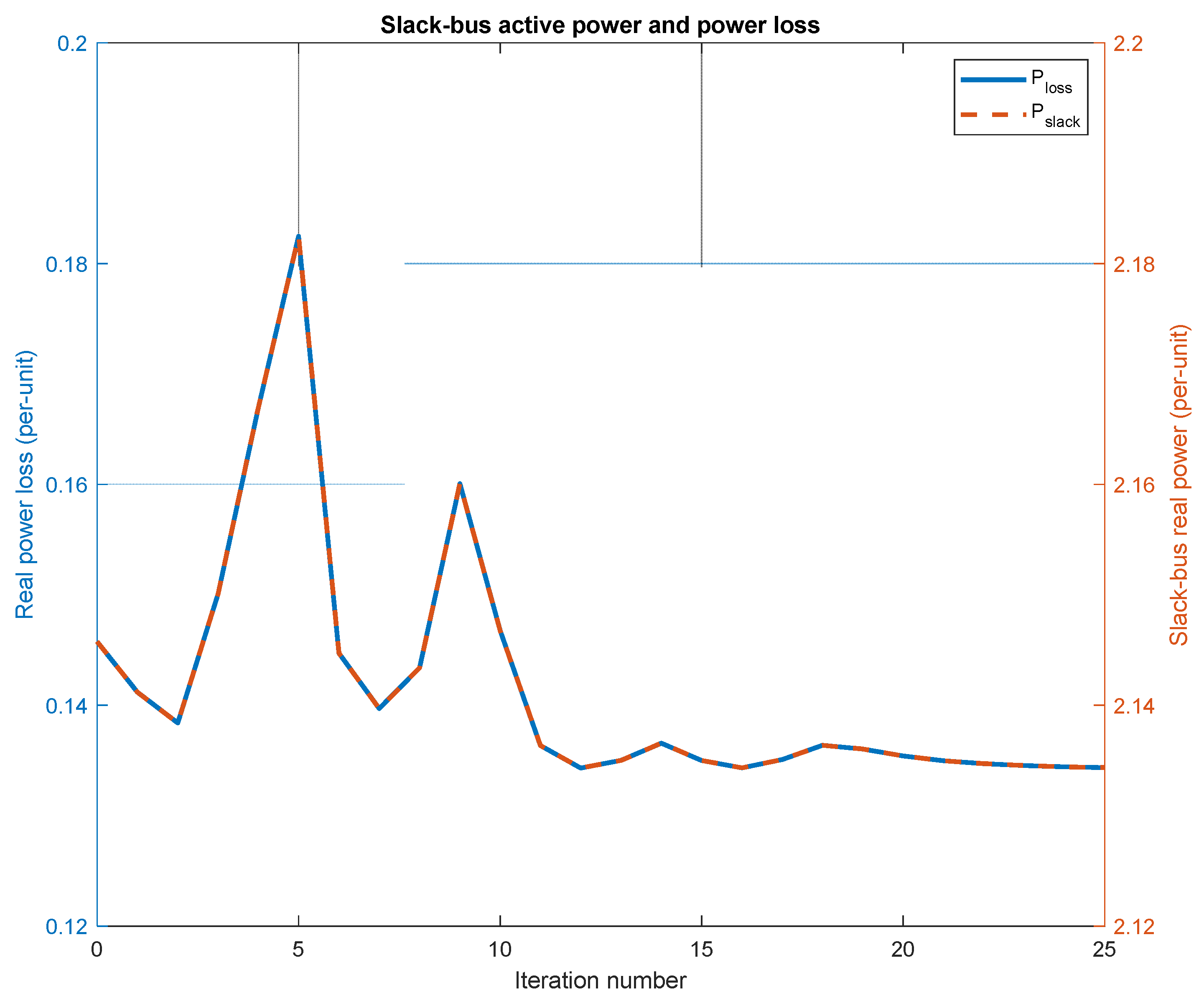
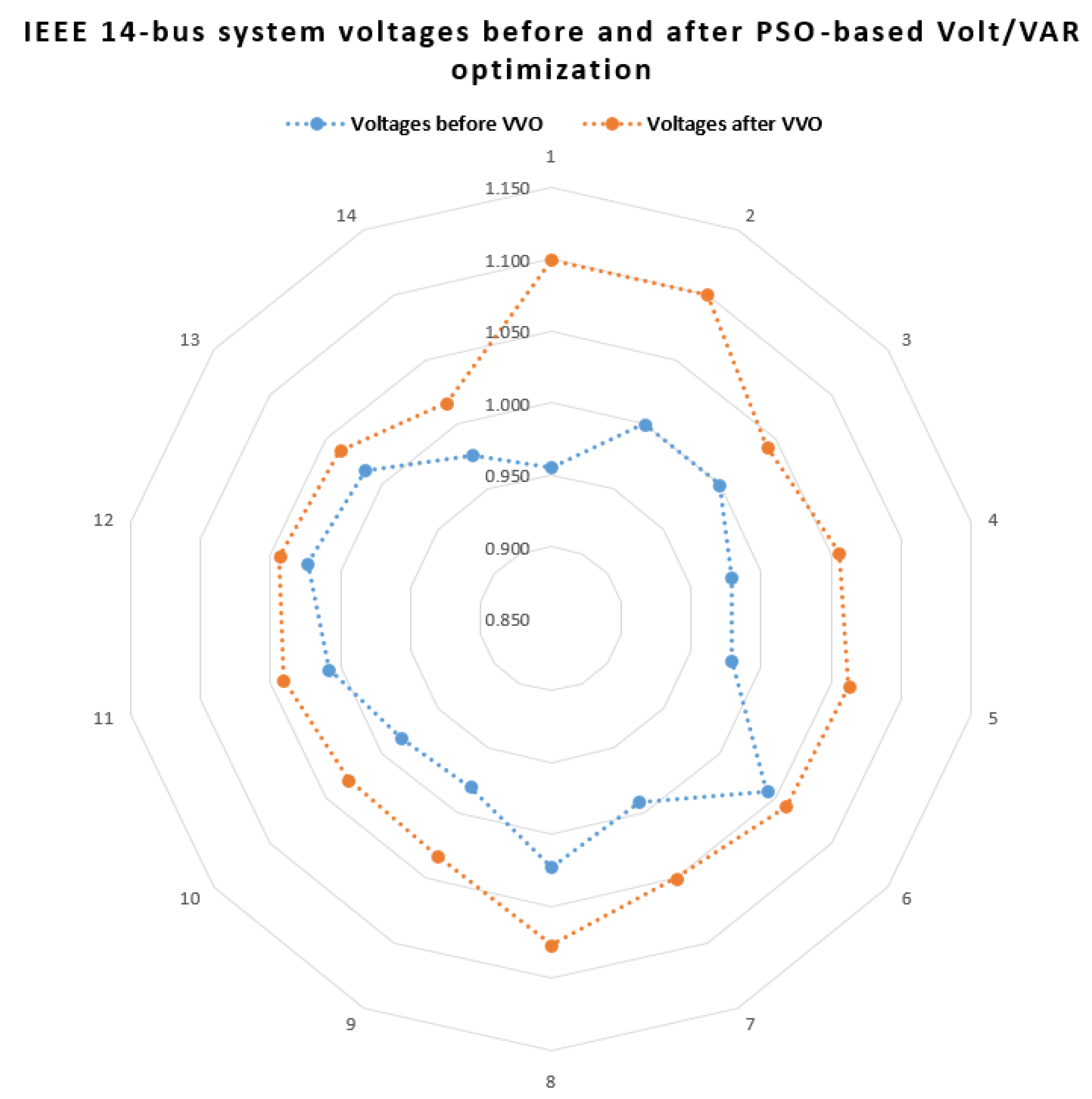
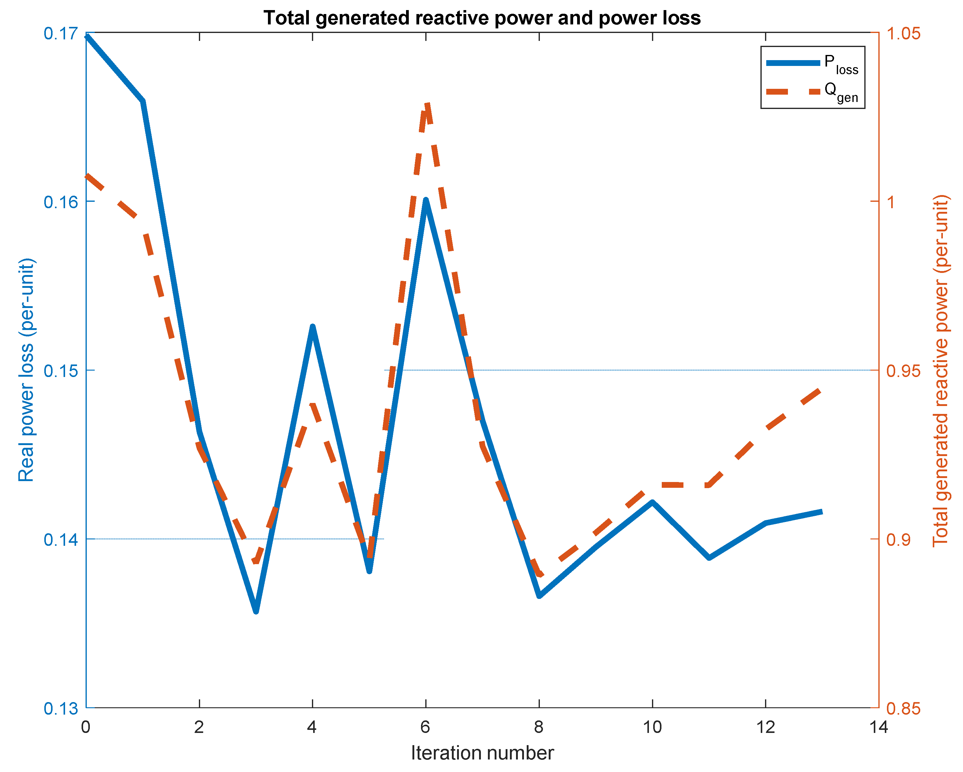
5.2.2. Case Study 2: IEEE 14-Bus Power System

The second case study is based on the IEEE 14-bus test system. The network, load, and generation data is taken from [34]. Results of applying the PSO algorithm to the 14-bus system for solving the VVO problem are presented in

Table 6. Summary of results of the PSO-VVO algorithm applied to the IEEE 14-bus power system.

Swarm Size	Initial Loss (p.u.)			Final Loss (p.u.)			Number of Iterations			Run Time (s)			Average % Loss Reduction
	Min	Max	Average	Min	Max	Average	Min	Max	Average	Min	Max	Average
10	0.1347	0.2011	0.1613	0.1235	0.1291	0.1279	6	40	21	0.0203	0.2432	0.1196	20.71
20	0.1353	0.1652	0.1439	0.1268	0.1290	0.1282	4	24	11	0.0214	0.1375	0.0662	10.91
30	0.1381	0.2408	0.1873	0.1290	0.1301	0.1293	5	71	41	0.0307	0.5822	0.2867	30.97
40	0.1416	0.1921	0.1613	0.1273	0.1290	0.1287	4	109	29	0.0237	0.6544	0.1791	20.22
50	0.1335	0.2385	0.1595	0.1290	0.1308	0.1294	5	51	21	0.0488	0.2931	0.1394	18.85

.

Based on the results presented in Table 6, the average real power loss reduction ranges from 10.91% in the case of the simulation with a swarm of 20 particles, to 30.97% in the case of the simulation with particle 30. The average number of iterations lies in the range between 11 and 41 for all cases. The minimum number of iterations is 4, recorded when the swarm size is 20 and 40, and the maximum number of iterations is 109, recorded in the case of a swarm size of 40. It can be noticed from the results presented in Table 6 that, while increasing the swarm size does not necessarily lead to increased execution time, there is a direct relationship between the number of iterations and the execution time. Thus, the maximum execution time (0.6544 s) is recorded in connection with the swarm size of 40, which also happens to coincide with the maximum number of iterations recorded for all the runs. The average execution time ranges from 0.0662 s (for a swarm size of 20) to 0.2867 s (for a swarm size of 30). The lowest absolute real power loss achieved is 0.1235 per unit, with a swarm size of 10. It can, thus, be seen here that the global minimum (in the context of the presented results) is attained with a swarm size of 10, implying that increasing the swarm size for this case does not necessarily lead to an improvement in the quality of the solution. It is worth noting that the (average) minimum number of iterations (11) is attained in the case of a swarm size of 20, which also has the minimum average execution time (0.0662 s).

The convergence behavior of the PSO algorithm for the 14-bus system is depicted in Figure 8 which, similar to Figure 4 for the 6-bus system, plots the changes in the global best position and in the fitness value of the global best position, as well as the fitness value of the global best position. This case takes a relatively shorter time period to converge, about 10 iterations, requiring about 0.05 s. It can be noticed that by the ninth iteration, the change in the global best position and the corresponding change in the fitness value of the global best position decrease to nearly zero, which signifies the satisfaction of the termination conditions for the algorithm.

The voltage profile of the 14-bus system before and after the Volt/VAR optimization is depicted in Figure 9 in the form of a radar chart. The post-optimization voltage magnitudes are greater than the pre-optimization values for all buses. It can be seen also for this case study that both the pre- and post-optimization voltages are within the range of nominal values (i.e., 0.95–1.1) for all the buses.

Figure 10 depicts the real power loss trajectory plotted together with the slack-bus active power output against the number of iterations. Similar to the 6-bus system case study, the close relationship between the change in the two quantities is clearly noticeable. Figure 11 compares the trajectories of the real power loss and the total generated system reactive power, which also depicts a relationship between the two quantities similar to that observed in the case of the real power loss and the slack-bus active power.

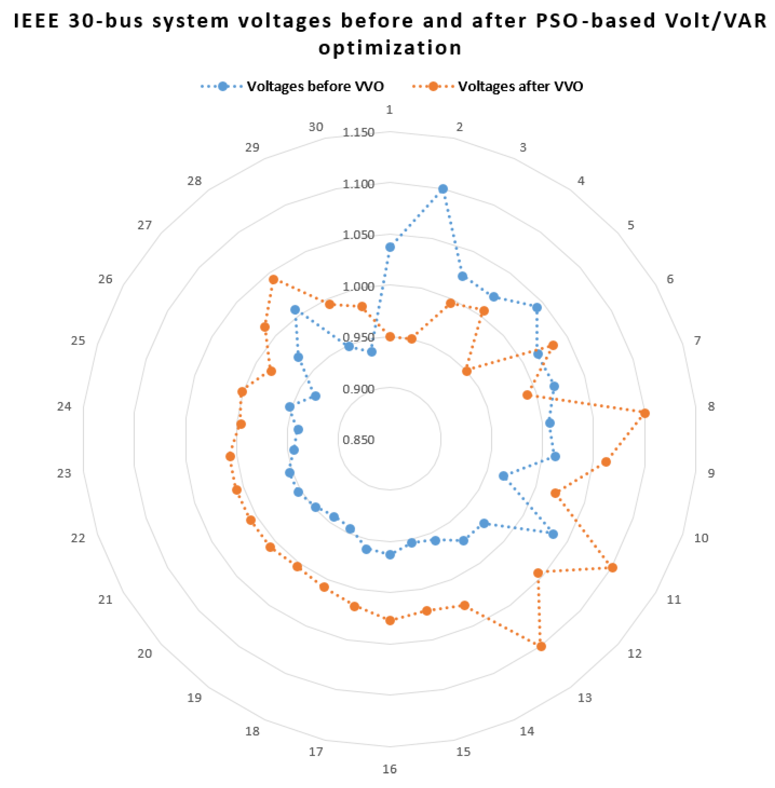
5.2.3. Case Study 3: IEEE 30-Bus Power System

The third case study is based on the IEEE 30-bus test system. It comprises 30 buses, 6 generators, 41 lines, and 21 loads. The network, load and generation data is also taken from [34]. Results of applying the PSO algorithm to the 30-bus system for solving the VVO problem are presented in

Table 7. Summary of results of the PSO-VVO algorithm applied to the IEEE 30-bus power system.

Swarm Size	Initial Loss (p.u.)			Final Loss (p.u.)			Number of Iterations			Run Time (s)			Average % Loss Reduction
	Min	Max	Average	Min	Max	Average	Min	Max	Average	Min	Max	Average
10	0.1353	2.0046	0.5253	0.0925	0.1067	0.0979	23	108	58	0.4386	2.1174	1.3169	81.29
20	0.1180	1.1763	0.4763	0.0925	0.0993	0.0947	32	179	80	0.7819	4.7353	2.2789	80.12
30	0.1203	0.8751	0.3089	0.0925	0.1054	0.0953	40	164	84	0.7581	3.7345	2.0272	69.15
40	0.1053	0.5211	0.2628	0.0925	0.0980	0.0937	20	170	96	0.4842	3.2412	1.6484	64.34
50	0.1008	1.1291	0.3987	0.0925	0.1031	0.0953	3	200	67	0.0448	4.8044	1.5187	76.10

.

The results presented in Table 7 show that there is substantial real power loss reduction in all the cases, ranging from 64.34% (attained with a swarm size of 20) to 81.29% (attained with a swarm size of 10). The average number of iterations is quite high for all the cases, lying in the range between 58 and 96. The dispersion between the minimum and maximum number of iterations is also quite high, the minimum and maximum values being 3 and 200 respectively, both obtained with a swarm size of 50. The average execution time ranges from a low of 1.3169 s to a high of 2.2789 s, obtained with swarm sizes of 10 and 20, respectively. Compared with the previous case studies, the 30-bus system requires significantly more iterations to converge and the execution time is correspondingly longer. As in the previous cases, increasing the swarm size does not seem to have a large impact on either the quality of the solution or the computational cost of the algorithm.

The convergence behavior of the PSO algorithm for the 30-bus system is depicted in Figure 12 and shows the changes in the global best position and in the fitness value of the global best position, as well as the fitness value of the global best position. The case depicted in the figure converges relatively quickly, requiring only about four iterations and an execution time of about 0.05 s.

The voltage profile of the 30-bus system before and after the Volt/VAR optimization is depicted in Figure 13 in the form of a radar chart. The post-optimization voltage magnitudes are greater than the pre-optimization values for the majority of buses. Some voltages hit their lower or upper limits, but there is no voltage violation for any of the buses.

Figure 14 plots the real power loss trajectory together with the slack-bus active power output against the number of iterations and Figure 15 does the same for the real power loss and total generated system reactive power trajectories. Similar characteristics can be observed as those observed in the preceding case studies.

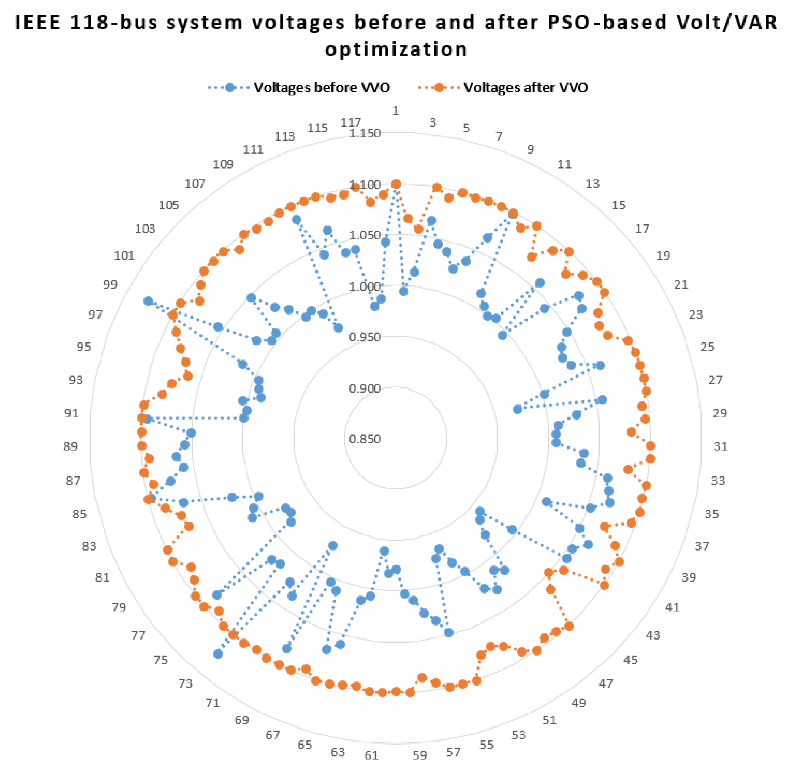
5.2.4. Case Study 4: IEEE 118-Bus Power System

The final case study considered is that of the IEEE 118-bus test system. It comprises 118 buses, 54 generators (35 of which are synchronous condensers), 186 lines, and 99 loads. The network, load, and generation data is taken from [35]. Results of applying the PSO algorithm to the 118-bus system for solving the VVO problem are summarized in

Table 8. Summary of results of the PSO-VVO algorithm applied to the IEEE 118-bus power system.

Swarm Size	Initial Loss (p.u.)			Final Loss (p.u.)			Number of Iterations			Run Time (s)			Average % Loss Reduction
	Min	Max	Average	Min	Max	Average	Min	Max	Average	Min	Max	Average
10	4.4286	6.7848	5.3158	2.3799	2.8516	2.6342	200	200	200	81.8725	82.7431	82.3317	50.45
20	5.0498	11.8646	7.9246	2.3778	3.0462	2.4514	111	200	183	45.7052	93.5918	77.8222	67.44
30	4.2654	11.0633	6.2787	2.3935	3.0599	2.5487	200	200	200	83.9581	88.0829	85.9590	59.41
40	4.4071	9.8267	5.9971	2.3822	2.5720	2.4510	200	200	200	82.2720	85.6926	84.2950	59.13
50	4.6573	11.1649	8.6517	2.3743	2.5027	2.4172	200	200	200	85.4243	86.8651	85.7809	72.06

.

The results for the 118-bus system presented in Table 8 show the average real power loss reduction among all the simulated cases to range from 50.45% (attained with a swarm size of 10) to 72.06% (attained with a swarm size of 50). The average number of iterations is quite high for all the cases. In fact, all cases except the case with a swarm size of 20 reach the pre-set maximum number of iterations. The average execution time is also quite high, especially when compared with the preceding case studies, and ranges from 77.8 s to 85.9 s. The minimum real power loss achieved is 2.37 per unit. The results are quite consistent over the range of the swarm size, implying that the algorithm’s performance is not significantly influenced by changing the swarm size, something that has been observed across all the preceding case studies as well.

The convergence behavior of the PSO algorithm for the 118-bus system is displayed in Figure 16, which depicts the changes in the global best position in the top trace and the fitness value of the global best position in the bottom trace of the figure. It can be seen from the figure that the algorithm exhibits oscillatory behavior beyond the 40th iteration. This also seems to explain the results tabulated in Table 8, the oscillatory behavior being the reason behind the algorithm exhausting the pre-set maximum number of iterations. By adjusting the tolerance value of the termination condition slightly higher (i.e., the change in the fitness value over successive iterations) the algorithm successfully terminates in much fewer iterations, as depicted in Figure 17.

The voltage profile of the 118-bus system before and after the Volt/VAR optimization is depicted in Figure 18 in the form of a radar chart. The pattern is similar to the preceding case studies, with the post-optimization voltage magnitudes being greater than the pre-optimization values for almost all the buses. Incidentally, the Volt/VAR optimization also alleviates some over-voltage conditions, particularly at buses 73 and 99, where the initial (i.e., pre-optimization) voltage magnitudes actually exceed the upper limit of 1.1 per unit.

6. Comparison of the PSO-Based with the PDIPM-Based Volt/VAR Optimization Algorithms

In this section, a comparative performance analysis is conducted between the PSO algorithm and the primal-dual interior-point method (PDIPM) as solution methods for the Volt/VAR optimization problem. The design and implementation of the PDIPM-based VVO algorithm has been presented by the authors in [20] and its performance analysis has been based on the same set of case studies as the ones used in this article. This has made the comparison relatively easier. The summary of the results of the comparison is detailed in

Table 9. Comparison of the PSO-VVO and PDIPM-VVO [20] algorithms applied to four case studies.

System	Initial Loss (p.u.)		Final Loss (p.u.)		Number of Iterations		Run Time (s)		% Loss Reduction
	PDIPM	PSO	PDIPM	PSO	PDIPM	PSO	PDIPM	PSO	PDIPM	PSO
6-bus	0.1335	0.1613	0.1290	0.1255	13	19	0.1775	0.0615	3.37	20.40
14-bus	0.1353	0.1613	0.1296	0.1235	14	21	0.1477	0.1596	4.24	23.43
30-bus	0.1141	0.1353	0.1084	0.0925	14	58	0.3565	1.3170	5.03	31.63
118-bus	3.3939	4.6573	3.2270	2.3743	8	200	2.0120	85.78	4.92	49.02

. For the PSO algorithm, since several simulations have been performed for each case study, a representative solution has been selected for comparison with the PDIPM algorithm, considering the performance evaluation criteria used in Table 9.

The comparative performance analysis is made on the basis of the computational efficiency, in terms of the number of iterations taken by the algorithm to converge and the execution time required, as well as the percentage real power loss reduction. As can be deduced from the table, the PSO algorithm far outperforms the PDIPM algorithm in terms of the percentage loss reduction in all cases, as it consistently achieves much higher percentage loss reduction, and the final per-unit loss reduction is less for the PSO algorithm in all cases. The computational efficiency of the PSO algorithm, however, is generally worse than that of the PDIPM algorithm. It requires a much higher number of iterations in order to converge in all cases, with the exception of the 6-bus system, which has a smaller execution time; although, the number of iterations taken by the algorithm to converge is still higher. The results seem to suggest that the computational cost of the PSO algorithm tends to increase significantly as the problem dimension increases. The results of this study demonstrate what is generally known about the relative performance characteristics of classical and heuristic optimization techniques. The main strength of classical optimization methods is their high computational efficiency, particularly for differentiable nonlinear systems, but they have the drawback of lacking the ability to find the globally optimal solution. Heuristic optimization techniques, on the other hand, generally incur high computational cost but have the advantage that they have the capability to find the globally optimal solution [37].

As an additional comparative performance analysis, the performance of the two algorithms developed and implemented by the authors in this and the companion article [20] is compared with some results presented in the literature for the IEEE 14-bus system. The results are summarized in

Table 10. Comparison of the PSO-VVO and PDIPM-VVO algorithms with other algorithms from the literature for the IEEE 14-bus system case study.

	Interior-Point Method ([34])	Linear Programming ([34])	PDIPM ([20])	PSO (Presented in This Article)
Initial loss (p.u.)	0.11646	0.11646	0.1125	0.1613
Final loss (p.u.)	0.11004	0.11108	0.1084	0.1235
% Real power loss reduction	5.513	4.619	6.914	23.43
Number of iterations	-	-	16	21
Execution time (s)	18.2	61.5	0.0578	0.1596

. It can be deduced from the comparative analysis that the PSO algorithm presented in this article exhibits superior performance in terms of solution quality (i.e., magnitude of percentage power loss reduction), whereas the PDIPM algorithm outperforms in terms of computational efficiency (i.e., required number of iterations for convergence and corresponding execution time).

7. Conclusions

This article has presented a detailed account of the design and implementation of the particle swarm optimization (PSO) algorithm for solving the Volt/VAR optimization (VVO) problem formulated in rectangular coordinates, as well as comparative analysis with the primal-dual interior-point method (PDIPM) for the solution of the same problem, which has been published by the authors in a companion article [20]. A brief presentation on the historical development of the PSO algorithm is followed by a discussion of the principle of operation and basic construction of the algorithm, after which some pertinent implementation aspects are presented. The adaptation of the algorithm to the solution of the VVO problem is then outlined, before presenting four case studies by means of which the performance analysis of the developed PSO algorithm has been analyzed. For each case study, a detailed qualitative and numerical analysis of the simulation results has been presented. The numerical results are tabulated in the respective sections where the case studies have been discussed. The comparative performance analysis of the PSO-VVO and PDIPM-VVO algorithms reveals that the PSO algorithm consistently achieves higher power loss reductions, as tabulated in Table 9. Thus, for instance, the percentage loss reduction is 20% for the PSO algorithm vs. 3% for the PDIPM in the case of the 6-bus system. The PDIPM, on the other hand, exhibits superior computational efficiency, as it requires fewer iterations to converge and lower execution time. This is especially the case for higher-dimensional systems. Thus, for instance, the PDIPM requires 14 iterations and 0.36 s to converge, whereas the PSO algorithm requires (on average) about 58 iterations and 1.32 s to converge, in the case of the IEEE 30-bus system. For a summary of the comparative analysis of the other case studies, reference may be made to Table 9. From the presented results, it can be deduced that the PSO algorithm outperforms the PDIPM in terms of real power loss reduction but underperforms in terms of computational efficiency, especially for higher-dimensional systems (such as the 118-bus system). Comparison of the developed algorithms with those published in the literature further reveals their superior performance in terms of computational efficiency and quality of the solution, as detailed in Table 10. The analysis of the PSO-VVO algorithm also reveals that increasing the swarm size does not necessarily result in a significant improvement in the solution quality for all the case studies considered. As indicated in Table 3, besides the maximum number of iterations, the absolute change in the fitness value of the global best position from one iteration to another has been used as an additional termination condition for this study. The algorithm is considered to have converged (and is, thus, terminated) if this change is insignificant over a number of iterations. Future work will look into the design and implementation of hybrid algorithms that seek to combine the synergistic characteristics of classical and heuristic optimization techniques.

References

1. Carpentier, J. Contribution a l’etude du dispatching economique. Bull. De La Soc. Fr. Des Electr. 1962, 3, 431–447. [Google Scholar]
2. Momoh, J.A. Electric Power System Applications of Optimization; Marcel Dekker Inc.: New York, NY, USA, 2001. [Google Scholar]
3. Papazoglou, G.; Biskas, P. Review and comparison of genetic algorithm and particle swarm optimization in the optimal power flow problem. Energies 2023, 16, 1152. [Google Scholar] [CrossRef]
4. Skolfield, J.K.; Escobedo, A.R. Operations research in optimal power flow: A guide to recent and emerging methodologies and applications. Eur. J. Oper. Res. 2022, 300, 387–404. [Google Scholar] [CrossRef]
5. Risi, B.-G.; Riganti-Fulginei, F.; Laudani, A. Modern techniques for the optimal power flow problem: State of the art. Energies 2022, 15, 6387. [Google Scholar] [CrossRef]
6. Mataifa, H.; Krishnamurthy, S.; Kriger, C. Volt/VAR optimization: A survey of classical and heuristic optimization methods. IEEE Access 2022, 10, 13379–13399. [Google Scholar] [CrossRef]
7. Ullah, Z.; Wang, S.; Wu, G.; Hasanien, H.M.; Jabar, M.W.; Qazi, H.S.; Tostado-Veliz, M.; Turky, R.A.; Elkadeem, M.R. Advanced studies for probabilistic optimal power flow in active distribution networks: A scientometric review. IET Gener. Transm. Distrib. 2022, 16, 3579–3604. [Google Scholar] [CrossRef]
8. Shen, Z.; Liu, M.; Xu, L.; Lu, W. Bi-level mixed-integer linear programming algorithm for evaluating the impact of load-redistribution attacks on Volt/VAR optimization in high- and medium-voltage distribution systems. Electr. Power Energy Syst. 2021, 128, 106683. [Google Scholar] [CrossRef]
9. Li, P.; Wu, Z.; Yin, M.; Shen, J.; Qin, Y. Distributed data-driven distributionally robust Volt/Var control for distribution network via an accelerated alternating optimization procedure. In Proceedings of the 3rd International Conference on Power Engineering (ICPE 2022), Sanya, China, 9–11 December 2022. [Google Scholar]
10. Papadimitrakis, M.; Kapnopoulos, A.; Tsavartzidis, S.; Alexandridis, A. A cooperative PSO algorithm Volt-VAR optimization in smart distribution grids. Electr. Power Syst. Res. 2022, 212, 108618. [Google Scholar] [CrossRef]
11. Tan, J.; He, M.; Zhang, G.; Liu, G.; Dai, R.; Wang, Z. Volt/Var Optimization for Active Power Distribution Systems on a Graph Computing Platform: An Paralleled PSO Approach. In Proceedings of the 2020 IEEE Power & Energy Society General Meeting (PESGM), Montreal, QC, Canada, 2–6 August 2020; pp. 1–5. [Google Scholar]
12. Quan, H.; Li, Z.; Zhou, T.; Yin, J. Two-stage optimization strategy of multi-objective Volt/Var coordination in electric distribution network considering renewable uncertainties. In Proceedings of the International Conference on Frontiers of Energy and Environment Engineering, CFEEE, Beihai, China, 16–18 December 2022. [Google Scholar]
13. Granados, J.F.L.; Uturbey, W.; Valadao, R.L.; Vasconcelos, J.A. Many-objective optimization of real and reactive power dispatch problems. Electr. Power Energy Syst. 2023, 146, 108725. [Google Scholar] [CrossRef]
14. Lian, L. Reactive power optimization based on adaptive multi-objective optimization artificial immune algorithm. Ain Shams Eng. J. 2022, 13, 101677. [Google Scholar] [CrossRef]
15. Vitor, T.S.; Vieira, J.C.M. Operation planning and decision-making approaches for Volt/Var multi-objective optimization in power distribution systems. Electr. Power Syst. Res. 2021, 191, 106874. [Google Scholar] [CrossRef]
16. Hossain, R.; Gautam, M.; Thapa, J.; Livani, H.; Benidris, M. Deep reinforcement learning assisted co-optimization of Volt-VAR grid service in distribution networks. Sustain. Energy Grids Netw. 2023, 35, 101086. [Google Scholar] [CrossRef]
17. Christy, A.A.; Vimal Raj, P.A.D. Adaptive biogeography based predator-prey optimization technique for optimal power flow. Electr. Power Energy Syst. 2014, 62, 344–352. [Google Scholar] [CrossRef]
18. Sulaiman, M.H.; Mustaffa, Z.; Mohamed, M.R.; Aliman, O. Using gray wolf optimizer for solving optimal reactive power dispatch problem. Appl. Soft Comput. 2015, 32, 286–292. [Google Scholar] [CrossRef]
19. Nocedal, J.; Wright, S.J. Numerical optimization, 2nd ed.; Springer Science+Business Media LLC.: New York, NY, USA, 2006. [Google Scholar]
20. Mataifa, H.; Krishnamurthy, S.; Kriger, C. An efficient primal-dual interior-point algorithm for Volt/VAR optimization in rectangular voltage coordinates. IEEE Access 2023, 11, 36890–36906. [Google Scholar] [CrossRef]
21. Taylor, G.A.; Song, Y.-H.; Irving, M.R.; Bradley, M.E.; Williams, T.G. A review of algorithmic and heuristic based methods for voltage/var control. In Proceedings of the 5th International Power Engineering Conference, Singapore; 2001; Volume 1, pp. 117–122. [Google Scholar]
22. Capitanescu, F.; Glavic, M.; Wehenkel, L. An interior-point based optimal power flow. In Proceedings of the 3-rd ACOMEN Conference, Ghent, Belgium, June 2005. [Google Scholar]
23. Kennedy, J.; Eberhart, R. Particle swarm optimization. In Proceedings of the ICNN’95-International Conference on Neural Networks, Perth, Australia, 27 November–1 December 1995; Volume 4, pp. 1942–1948. [Google Scholar]
24. Reynolds, C. Flocks, herds and schools: A distributed behavioral model. Comput. Graph. 1987, 21, 25–34. [Google Scholar] [CrossRef]
25. Heppner, F.; Grenander, U. A stochastic nonlinear model for coordinated bird flocks. In The Ubiquity of Chaos; Krasner, S., Ed.; AAAS Publications: Washington, DC, USA, 1990. [Google Scholar]
26. Hu, X.; Shi, Y.; Eberhart, R. Recent advances in particle swarm. In Proceedings of the 2004 congress on evolutionary computation, Portland, OR, USA, 19–23 June 2004; Volume 1, pp. 90–97. [Google Scholar]
27. Poli, R.; Kennedy, J.; Blackwell, T. Particle swarm optimization: An overview. Swarm Intell. 2007, 1, 33–37. [Google Scholar] [CrossRef]
28. Talukder, S. Mathematical modeling and applications of particle swarm optimization. Master’s Thesis, Blekinge Institute of Technology, Karlskrona, Sweden, 2011. [Google Scholar]
29. Freitas, D.; Lopes, L.G.; Morgado-Dias, F. Particle swarm optimization: A historical review up to the current developments. Entropy 2020, 22, 362. [Google Scholar] [CrossRef] [PubMed]
30. Shi, Y.; Eberhart, R. A modified particle swarm optimizer. In Proceedings of the 1998 IEEE International Conference on Evolutionary Computation Proceedings, Anchorage, AK, USA, 4–9 May 1998; pp. 69–73. [Google Scholar]
31. Clerc, M.; Kennedy, J. The particle swarm—Explosion, stability and convergence in a multidimensional complex space. IEEE Trans. Evol. Comput. 2002, 6, 58–73. [Google Scholar] [CrossRef]
32. MATLAB; Version 2023a; The MathWorks Inc.: Natick, MA, USA, 2023.
33. Wood, A.J.; Wollenberg, B.F.; Sheble, G.B. Power Generation, Operation and Control, 3rd ed.; John Wiley & Sons, Inc.: Hoboken, NJ, USA, 2014. [Google Scholar]
34. Zhu, J. Optimization of Power System Operation; John Wiley and Sons, Inc.: Hoboken, NJ, USA, 2009. [Google Scholar]
35. Springer Verlag. Appendix E: IEEE 118-bus Test System Data. 2012. Available online: https://link.springer.com/content/pdf/bbm%3A978-1-4615-4473-9%2F1.pdf (accessed on 23 January 2023).
36. Kundur, P. Power System Stability and Control; McGraw Hill Inc.: New York, NY, USA, 1994. [Google Scholar]
37. Frank, S.; Stepanovice, I.; Rebennack, S. Optimal power flow: A bibliographic survey II, nondeterministic and hybrid methods. Energy Syst. 2012, 3, 259–289. [Google Scholar] [CrossRef]
Figure 1. Summary of the key developments of the particle swarm optimization algorithm over the years.
Mathematics 11 04093 g001
Figure 2. Flowchart of the standard PSO algorithm.
Mathematics 11 04093 g002
Figure 3. Flowchart of the PSO algorithm applied to the VVO problem.
Mathematics 11 04093 g003
Figure 4. Convergence characteristics of the PSO algorithm applied to the 6-bus system.
Mathematics 11 04093 g004
Figure 5. Change in voltage profile of the 6-bus system due to PSO-based VVO.
Mathematics 11 04093 g005
Figure 6. Real power loss and slack-bus generated power of the 6-bus system plotted against the number of iterations of the PSO-based VVO algorithm.
Mathematics 11 04093 g006
Figure 7. 6-bus system real power loss and total system reactive power generation plotted against the number of iterations of the PSO-based VVO algorithm.
Mathematics 11 04093 g007
Figure 8. Convergence characteristics of the PSO algorithm applied to the IEEE 14-bus system.
Mathematics 11 04093 g008
Figure 9. Change in voltage profile of the IEEE 14-bus system due to PSO-based VVO.
Mathematics 11 04093 g009
Figure 10. IEEE 14-bus system real power loss and slack-bus generated power plotted against the number of iterations of the PSO-based VVO algorithm.
Mathematics 11 04093 g010
Figure 11. IEEE 14-bus system real power loss and total system reactive power generation plotted against the number of iterations of the PSO-based VVO algorithm.
Mathematics 11 04093 g011
Figure 12. Convergence characteristics of the PSO algorithm applied to the IEEE 30-bus system.
Mathematics 11 04093 g012
Figure 13. Change in voltage profile of the IEEE 30-bus system due to PSO-based VVO.
Mathematics 11 04093 g013
Figure 14. IEEE 30-bus system real power loss and slack-bus generated power plotted against the number of iterations of the PSO-based VVO algorithm.
Mathematics 11 04093 g014
Figure 15. IEEE 30-bus system real power loss and total system reactive power generation plotted against the number of iterations of the PSO-based VVO algorithm.
Mathematics 11 04093 g015
Figure 16. Convergence characteristics of the PSO algorithm applied to the IEEE 118-bus system.
Mathematics 11 04093 g016
Figure 17. Convergence characteristics of the PSO algorithm applied to the IEEE 118-bus system after adjusting the tolerance higher.
Mathematics 11 04093 g017
Figure 18. Change in voltage profile of the IEEE 118-bus system due to PSO-based VVO.
Mathematics 11 04093 g018