An Innovative Approach to Predict the Diffusion Rate of Reactant’s Effects on the Performance of the Polymer Electrolyte Membrane Fuel Cell

Abstract

As the analytical solution can provide much more accurate and reliable results in a short time, in the present study, an innovative analytical approach based on the perturbation method is proposed. The governing equations, which consist of continuity, momentum, species, and energy equations, are solved analytically by using the regular perturbation method. The perturbation parameter is the function of the penetration (diffusion) velocity. At first, the momentum and continuity equations are coupled together and solved analytically to find the velocity distribution. In the polymer electrolyte membrane fuel cell (PEMFC), the penetration velocity can be increased by increasing the gas diffusion layer (GDL) porosity and the operating pressure of the PEMFC. The solution showed that by increasing the perturbation parameter from 0 to the higher values, the diffusion of the reactant toward the gas channel to the GDL is improved too, leading to the enhancement of the performance of the PEMFC. The axial velocity profile tends to the bottom of the flow channel. This fact helps the reactant to transfer into the reaction area quickly. For perturbation parameter 0.5, in the species equation, the distribution of species in the reaction areas is more regular and uniform. For the lower magnitudes of the Peclet number, the species gradient is enhanced, and as a result, the concentration loss takes place at the exit region of the channel. Also, increasing the perturbation parameter causes an increase in the temperature gradient along the flow channel. For higher perturbation parameters, there is a higher temperature gradient from the bottom to the top of the track in the flow direction. The temperature profile in the y direction has a nonlinear profile at the inlet region of the channel, which is converted to the linear profile at the exit region. To verify the extracted analytical results, the three-dimensional computational fluid dynamic model based on the finite volume method is developed. All of the achieved analytical results are compared to the numerical ones in the same condition with perfect accordance.

1. Introduction

Energy provision is one of the main concerns of humanity today. Currently, fossil fuels are one of the primary sources of energy supply. The most crucial problem with fossil fuels is their perishability. The next issue about these fuels is that they cause environmental pollution (global warming, climate change, melting polar ice caps, acid rain, pollution, damage to the ozone layer, etc.) [1,2,3]. Using clean and renewable energies instead of limited fossil energy can help to solve these challenges. Hydrogen energy is one of these clean energies that can supply future energy resources like electricity for domestic and industrial use, transportation energy, etc. [4]. Among the different kinds of hydrogen energy, polymer electrolyte membrane fuel cells (PEMFCs) have the maximum power density and efficiency, low operational temperature, environmental compatibility, and no pollution. These advantages make the PEMFC the best candidate for obtaining energy from hydrogen energy [5,6]. Nowadays, the establishment of PEMFC systems to supply energy to vehicles has grown significantly in the automotive industry [7,8,9,10]. In recent years, research and development on fuel cells and systems have been greatly accelerated; nevertheless, the cost of the fuel cell system is still very high and cannot make it a long-term commercial product [11,12].

Because of the importance of the PEMFC’s role in the future energy resource supply, many researchers have focused on various aspects of fuel cell performance enhancement. Chu and Jiang [13] modeled an air-breathing stack and evaluated the performance of this type of stack. Moore et al. simulated a battlefield contaminant on the performance of the PEMFC, and they concluded that these types of contaminants do not affect the PEMFC performance [14]. Hamelin et al. [15] considered the dynamic behavior of fuel cell performance enhancement and compared their experimental results with Mann et al. [16]. As can be seen, the main vital parameters to enhance the performance of the PEMFC are its optimizations of geometrical and operational conditions.

There are a lot of investigations that suggest 2D and 3D numerical models based on the computational fluid dynamic (CFD) methods. Tao et al. [17] simulated the performance of a metal foam pattern flow field for PEMFC. In this way, the performance of the fuel cell has a significant enhancement, especially at higher current densities of about 5% at the same condition. Qin et al. [18] developed a new two-block structure flow channel three-dimensional model. They showed that increasing the number of blocks to six can increase the performance of the fuel cell significantly. Also, this new design could improve the liquid water removal from the cathode side. The effect of a distributed magnetic field on the output power of the PEMFC is studied by Mao et al. [19]. This work indicated the magnetic field benefits to PEMFC performance and the water flooding phenomena. Also, Chen et al. suggested a numerical model that predicts the behavior of fuel cell performance with consideration of the thermal resistance of the interfaces [20]. Increasing the roughness of the surface from 1 µm to 3 µm increases the current density up to 17.7%. Cheng et al. proposed a numerical model that simulated the wave-like gas channel. This fuel cell had a groove on the gas diffusion layers. This geometrical configuration leads to a net performance increase of about 2.64% in the PEMFC [21].

The novel design of the high-temperature PEMFC is modeled by Duan et al. [22] and Ni et al. [23]. Chen et al. [24] investigated the effects of the dead-ended channel on the performance of the PEMFC. This type of channel causes a more uniform distribution of current density in the PEMFC. Jiao and Zhang [25] developed a three-dimensional multiphase for a PEMFC that could predict the effect of the wave-like channel on the cell’s performance. These types of gas channels help to remove water from the PEMFCs. Ranjbar et al. [26] designed and numerically simulated a model with a metal bipolar plate and an innovative cooling field. They found out that by using the 5% vol nano-fluid, they could achieve the desired cooling in the Reynolds 500. Qin et al. [27] numerically investigated the mass transport phenomena with the baffle plates installed in the channel. In this study, they also investigated the optimum number of baffles. Considering this fact, the numerical models, which are modeled with computer-based programs, have such a high computational cost. If a higher-precision model is needed, the development of a 3D model is inevitable. Three-dimensional CFD models are difficult to develop and require highly time-consuming procedures to obtain an accurate answer. Also, this kind of model has limitations and sometimes has less-accurate results compared with the physics of the problem. Therefore, this kind of result should be validated by experimental or analytical results.

Lately, experimental results have been developed to examine the performance of the PEMFC in different operational conditions. For instance, Tai et al. [28] designed an experimental setup to predict the temperature behavior of the PEMFC in a CCHP cycle. In another work, Li et al. [29] studied the effect of the flow channel parameters on the durability of a PEMFC stack. They found that the lowest performance of the cell is for the shallow flow channel. This kind of channel leads to severe voltage drop. Also, hydrogen consumption, in this case, is increased in the long-term use of the PEMFC. The experimental setup devices are expensive, and for highly accurate results, highly accurate devices with less uncertainty should be presented. Also, experimental analysis has a high procedure time to obtain results. In a case with numerous parameters, it takes considerable time to obtain the results, and it is expensive to study a large number of parameters to find the optimal one.

A little while back, analytical solutions to the governing equations in physical and engineering problems have been expanded widely. These kinds of solutions can predict the problem easily, precisely, and in a less time-consuming procedure. However, there are some limitations in the analytical solution of the nonlinear equations. This fact results in the number of analytical solutions in the modeling of the PEMFC phenomena being low, and most of these works just modeled the electrochemical equations or just introduced a simple analytical model with low accuracy. Chang et al. [30] developed an analytical model to predict oxygen transport in the PEMFC. They showed that the concentration of oxygen in the gas diffusion layers (GDLs) is highly dependent on the porosity and the thickness of this layer because, in a thick layer, the resistance against oxygen transport is increased significantly. Neyerlin et al. [31] studied the voltage loss in the catalyst layer in the PEMFC. As a result, they plotted the voltage loss as a function of the resistance of the catalyst layer. Haji [32] introduced an analytical model that predicted the three mail activation, ohmic, and concentration losses in the PEMFC. Also, in this work, the effect of the temperature on the cell performance was examined. Ahmadi et al. [33], by using the perturbation method, solved the governing equation to predict the velocity distribution in the different aspect ratios of the elliptical PEMFC. Also, in this work, they considered the diffusion rate for a cylindrical type of PEMFC. Chen et al. [34] suggested an analytical model and studied the PEMFC operational condition parametrically. In another work, Ahmadi and Kõrgesaar [35] used the perturbation method to solve the governing equation to plot the distribution of the velocity, species, and temperature in a trapezoidal flow channel. They concluded that inverse trapezoidal channels can increase the performance of the cell. Kulikovsky [36], by using a simple analytical model, could simulate the concentration impedance of the oxygen in the PEMFC. As can be mentioned, there are a few works that have used the mathematical solution to model the PEMFC.

In the present work, by using the regular perturbation method [37,38], the governing equations of fluid flow, which consists of continuity, momentum, species, and energy, are solved to model the distribution of the velocity, species, and temperature. The novelty of the work is the consideration of the penetration velocity of the species as the perturbation parameter. The penetration velocity of the species from the bottom of the flow channel, which is the function of the porosity of the GDLs and the operating pressure in the channel, is one of the key parameters that determine the performance value (output voltage in the same current density) of the PEMFC.

2. Mathematical Model

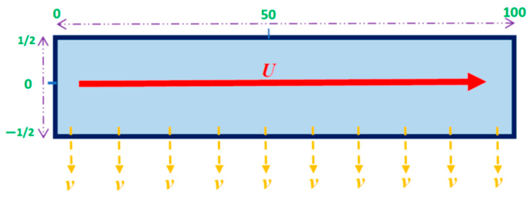
2.1. Model Assumption and Description

• In the PEM fuel cell, because of low flow velocity, it is expected that the Reynolds number would be less than 200 [35,38].
• Because of the low Mach number, the flow is assumed to be incompressible and laminar [38].
• Due to a low Reynolds, the flow can be supposed to be fully developed and 2D [35].
• Also, the penetration velocity of the species is dependent on the Faraday coefficient, current density value, and the distribution concentration of the species [35]. Underneath the regular operation of the PEM fuel cell, the current density should be about 1 A/cm². The mean value of the axial velocity of the reactant in the flow channels varies from 1 to 5 m/s, which is greater than the penetration velocity of the reactant from the bottom of the channel to the GDL (Equation (1)). The maximum magnitude of the penetration velocity is 0.001 m/s [33,35].

$$\left|v\right|=g\left(\frac{I}{F\cdot C_i}\right)\underset{}{\overset{}{⟶}}\frac{v}{U}=g\left({10}^{-3}\right)\stackrel{}{⟶}\frac{\partial }{\partial y}>>\frac{\partial }{\partial x}$$

(1)

where F is the Faraday coefficient, C is the concentration of species, v is the diffusion (penetration) velocity of species, and U is the average magnitude of the axial velocity. Hereupon, the term of pressure gradient in the momentum equation can be assumed to have a permanent magnitude.

In this case, the gas channel is rectangular. For finding the velocity distribution, the momentum equation will be solved using the perturbation method, considering the diffusion velocity as the perturbation parameter. Figure 1 shows the nondimensional scale of the flow channel from the side view.

2.2. Solving the Momentum Equation to Find the Velocity Distribution

The dimension of the gas channel is nondimensionalized by the gas channel height (h), which is 1 mm. The origin of the coordinate system in the y direction is posed in the middle of the channel inlet (y is assumed to be half of the gas channel height, as shown in Figure 1). The considered boundary conditions can be written as Equation (2):

$$\begin{array}{c}x=\frac{\widehat{x}}{h},\hspace{0.17em}\hspace{0.17em}y=\frac{\widehat{y}}{h}\\ u(\frac{1}{2})=0,\hspace{0.17em}\hspace{0.17em}u(-\frac{1}{2})=0, v(\frac{1}{2})=0, v(-\frac{1}{2})=-{v^{\prime }}_s\end{array}$$

(2)

For converting the parameters to the nondimensional form, the following terms are applied in the governing equations, which have been written in Equation (3) [35]:

$$u=\frac{\widehat{u}}{U}, v=\frac{\widehat{v}}{U}, P=\frac{\widehat{P}}{\rho U^2}, C=\frac{\overline{C}-C_{0A}}{C_{0A}-C_{\infty }}$$

(3)

The equations of continuity (Equation (4)) and momentum (Equation (5)) are as follows [35,38]:

$$\frac{\partial u}{\partial x}+\frac{\partial v}{\partial y}=0$$

(4)

$$u\frac{\partial u}{\partial x}-v\frac{\partial v}{\partial y}=-\frac{\partial P}{\partial x}+\frac{1}{Re}\frac{{\partial }^{2}u}{\partial y^2}$$

(5)

As the penetration velocity is assumed to be constant, so, according to the continuity equation, the following assumption can be made. Therefore, the flow can be assumed to be fully developed, as shown in Equation (6).

$$\frac{\partial v}{\partial y}=0\Rightarrow \frac{\partial u}{\partial x}=0$$

(6)

2.2.1. Determining the Perturbation Parameter

The perturbation parameter is defined as Equation (7). Since the diffusion velocity and, consequently, the Reynolds number are small, their product will be very small too. In this case, the obtained parameter can be considered as the perturbation parameter (ε) (Equation (8)).

$$\epsilon =-v_s\times Re$$

(7)

$$-v_s.Re\frac{\partial u}{\partial y}=-Re\frac{\partial P}{\partial x}+\frac{{\partial }^{2}u}{\partial y^2} \to \epsilon \frac{\partial u}{\partial y}=-\lambda +\frac{{\partial }^{2}u}{\partial y^2}$$

(8)

2.2.2. Velocity Distribution Definition Procedure

The velocity (u) profile is presented below as Equation (9), and it is replaced in Equation (10):

$$u=u_0+\epsilon u_1+{\epsilon }^2{u}_2+\dots$$

(9)

Substituting the velocity profile into Equation (8) results in:

$$\epsilon \frac{d}{dy}\left(u_0+\epsilon u_1+{\epsilon }^2{u}_2+{\epsilon }^3{u}_3+\dots \right)=-\lambda +\frac{d^2}{d{y}^2}\left(u_0+\epsilon u_1+{\epsilon }^2{u}_2+{\epsilon }^3{u}_3+\dots \right)$$

(10)

Now, we sort the parameters according to the power of ε (Equations (11)–(14)):

$$\begin{array}{c}{\epsilon }^0:\frac{d^2{u}_0}{d{y}^2}=\lambda \Rightarrow u_0=\frac{1}{2}\lambda y^2+c_{1}y+c_2\Rightarrow c_2=-\frac{\lambda }{2},c_1=0 \to \\ u_0=\frac{\lambda }{2}\left(y^2-1\right)\Rightarrow u_0=\frac{3}{2}\left(1-y^2\right)\end{array}$$

(11)

$$\begin{array}{c}{\epsilon }^1: \frac{d{u}_0}{dy}=\frac{d^2{u}_1}{d{y}^2}\Rightarrow \frac{d^2{u}_1}{d{y}^2}=\lambda y\Rightarrow \frac{d{u}_1}{dy}=\frac{\lambda }{2}{y}^2+c_3\\ \to u_1=\frac{\lambda }{6}{y}^3+c_{3}y+c_4\Rightarrow c_4=0,c_3=-\frac{\lambda }{6}\\ \to u_1=\frac{\lambda }{6}\left(y^3-y\right)\Rightarrow u_1=\frac{1}{2}\left(y-y^3\right)\end{array}$$

(12)

$$\begin{array}{c}{\epsilon }^2:\frac{d{u}_1}{dy}=\frac{d^2{u}_2}{d{y}^2}\Rightarrow \frac{d^2{u}_2}{d{y}^2}=\frac{\lambda }{6}(3y^2-1)\\ \frac{d{u}_2}{dy}=\frac{\lambda }{6}{y}^3-\frac{\lambda }{6}y+c_5\Rightarrow u_2=\frac{\lambda }{24}{y}^4-\frac{\lambda }{12}{y}^3+c_{5}y+c_6\\ c_5=0 , c_6=\frac{\lambda }{24}\\ u_2=\frac{\lambda }{24}\left(y^4-2y^2+1\right)\Rightarrow u_2=\frac{1}{8}\left(2y^2-y^4-1\right)\end{array}$$

(13)

$$\begin{array}{c}{\epsilon }^3:\frac{d{u}_2}{dy}=\frac{d^2{u}_3}{d{y}^2}=\frac{\lambda }{6}(y^3-y)\Rightarrow \frac{d{u}_3}{dy}=\frac{\lambda }{24}{y}^4-\frac{\lambda }{12}{y}^2+c_7\Rightarrow u_3=\frac{\lambda }{120}{y}^5-\frac{\lambda }{36}{y}^3+c_{7}y+c_8\\ c_8=0, c_7=\frac{\lambda }{90}\\ u_3=\frac{\lambda }{120}{y}^5-\frac{\lambda }{36}{y}^3+\frac{\lambda }{90}y\Rightarrow u_3=-\frac{1}{40}{y}^5+\frac{1}{12}{y}^3-\frac{1}{30}y\end{array}$$

(14)

To find λ, we proceed as in Equation (15):

$$1\approx \frac{1}{2}{\displaystyle \underset{-1}{\overset{1}{\int }}{u}_0}dy=\frac{1}{2}{\displaystyle \underset{0}{\overset{1}{\int }}\frac{\lambda }{2}\left(y^2-1\right)dy=\frac{\lambda }{4}}{\left(\frac{1}{3}{y}^3-y\right)}_0^1\Rightarrow \lambda =-3$$

(15)

Therefore, the velocity, in general, by the combination of the terms that are presented above, is equal to Equation (16):

$$u=\frac{3}{2}\left(1-y^2\right)+\frac{\epsilon }{2}\left(y-y^3\right)+\frac{{\epsilon }^2}{8}\left(2y^2-y^4-1\right)+{\epsilon }^3\left(-\frac{1}{40}{y}^5+\frac{1}{12}{y}^3-\frac{1}{30}y\right)+\dots$$

(16)

2.2.3. Comparison of Numerical and Analytical Results

For validating the results obtained from the analytical solution using the perturbation method, a comparison was made between the results extracted from the mentioned method and the data of the numerical model, which has been performed by the 3D computational fluid dynamic (CFD) technique based on the finite volume method, in the same boundary conditions. The numerical model is a general model that has been used in many previously published works and can calculate all of the properties of the PEMFC such as the transport phenomena, temperature, and charge distribution and the voltage–current density [1]. The mentioned numerical model in this study is used to validate the analytical results.

The perturbation parameters are considered as 0 and 0.7, while the perturbation parameter is equal to the product of the vertical component of the velocity (diffusion velocity of the species) in the Reynolds number. Also, the Reynolds number is constant and equal to Re = 200, so only the influence of changes in diffusion velocity is considered.

Figure 2 provides a comparison between the analytical and numerical results. According to the figure, it is clear that there is good agreement between them. The figure indicates that by increasing the value of the perturbation parameter, the difference between the analytical and numerical results changes slightly (the error is presented in

Table 1. Error comparison of the numerical and analytical results for momentum equation.

	Perturbation Parameter	Error $\left(\frac{\mathit{n}\mathit{u}\mathit{m}\mathit{e}\mathit{r}\mathit{i}\mathit{c}\mathit{a}\mathit{l}-\mathit{a}\mathit{n}\mathit{a}\mathit{l}\mathit{y}\mathit{t}\mathit{i}\mathit{c}\mathit{a}\mathit{l}}{\mathit{n}\mathit{u}\mathit{m}\mathit{e}\mathit{r}\mathit{i}\mathit{c}\mathit{a}\mathit{l}}\times \mathbf{100}\right)$
1	ε = 0	0.014
2	ε = 0.7	1.51

).

It should be noted that the range of diffusion velocity in a fuel cell varies from 0.0001 to 0.001. The Reynolds number is between 5 and 200. Therefore, the value of the perturbation parameter is between 0.0005 and 0.2, which is much less than one and fulfills the necessary condition to be selected as a perturbation parameter.

2.2.4. Analytical Results for Different Perturbation Parameters

Figure 3 shows the analytical results obtained from solving the momentum equation in the gas channel by the perturbation method for different perturbation parameters. By carefully examining Figure 3, it can be seen that with the increase in the penetration velocity or the vertical component of the velocity, the extreme point of the velocity distribution curve tends to the bottom of the gas channel, and at the same time, the value of this point decreases. In other words, with the increase in the penetration rate in the channel, the axial velocity decreases, and the penetration rate of reactive gases increases by the same amount. This causes an increase in the rate of penetration of species and probably increases the performance of the fuel cell.

2.3. Solving the Species Conservation Equation by Considering the Diffusion from the Gas Channel

For finding the concentration distribution, we choose the velocity term u₀ (which is the dominant term) and put it in the species conservation equation (Equation (17)).

$$\begin{array}{c}u\approx u_0=\frac{3}{2}\left(1-y^2\right)\\ u\frac{\partial C}{\partial x}+v\frac{\partial C}{\partial y}=\frac{1}{ReSc}\frac{{\partial }^{2}C}{\partial y^2}\Rightarrow \frac{3}{2}\left(1-y^2\right)\frac{\partial C}{\partial x}-v_s\frac{\partial C}{\partial y}=\frac{1}{ReSc}\frac{{\partial }^{2}C}{\partial y^2}\end{array}$$

(17)

Now, we make the concentration equation and the boundary conditions of the problem dimensionless to find the perturbation parameter. The boundary conditions of the species are given as Equation (18):

$$C (0, y)=0, {\left(\frac{\partial C}{\partial y}\right)}_{y=-\frac{1}{2}}=A {\left(\frac{\partial C}{\partial y}\right)}_{y=\frac{1}{2}}=0$$

(18)

According to the nondimensional equation of species conservation, the perturbation parameter (β) is defined as Equation (19):

$$-v_s.Re.Sc=\beta , Re=\frac{\rho ux}{\mu }, Sc=\frac{\mu }{\rho D}$$

(19)

where µ is the dynamic viscosity, ρ is the density, D is the mass permeability, Re is the dimensionless Reynolds number, and Sc is the dimensionless Schmidt number. The Schmidt number ranges from 0.56 to 0.76, and the Reynolds range is 5 to 200. The velocity also varies from 0.0001 to 0.001 m/s. Therefore, the value of the mentioned parameter is between 0.00027 and 0.152, which is much smaller than 1.

2.3.1. Solving the Species Conservation Equation

By assuming the species concentration profile as Equation (20) and substituting it into Equation (17), we have the following procedures (Equation (21)):

$$C=C_0+{\beta C}_1+{\beta }^2{C}_2+\dots \frac{3}{2}Re.Sc=k$$

(20)

$$\begin{array}{l}k\left(1-y^2\right)\frac{\partial C}{\partial x}-\beta \frac{\partial C}{\partial y}=\frac{{\partial }^{2}C}{\partial y^2}\Rightarrow k\frac{\partial C}{\partial x}-k{y}^2\frac{\partial C}{\partial x}-\beta \frac{\partial C}{\partial y}=\frac{{\partial }^{2}C}{\partial y^2}\\ k\frac{\partial }{\partial x}\left(C_0+\beta C_1+{\beta }^2{C}_2+\dots \right)-k{y}^2\frac{\partial }{\partial x}\left(C_0+\beta C_1+{\beta }^2{C}_2+\dots \right)\\ -\beta \frac{\partial }{\partial y}\left(C_0+\beta C_1+{\beta }^2{C}_2+\dots \right)=\frac{{\partial }^2}{\partial y^2}\left(C_0+\beta C_1+{\beta }^2{C}_2+\dots \right)\end{array}$$

(21)

If Equation (21) is arranged according to the different powers of the perturbation parameter, then Equations (22)–(24) are achieved:

$${\beta }^0:k\frac{\partial C_0}{\partial x}-k{y}^2\frac{\partial C_0}{\partial x}=\frac{{\partial }^2{C}_0}{\partial y^2}\Rightarrow k\left(1-y^2\right)\frac{\partial C_0}{\partial x}=\frac{{\partial }^2{C}_0}{\partial y^2}$$

(22)

$${\beta }^1:k\frac{\partial C_1}{\partial x}-k{y}^2\frac{\partial C_1}{\partial x}-\frac{\partial C_0}{\partial y}=\frac{{\partial }^2{C}_1}{\partial y^2}\Rightarrow k\left(1-y^2\right)\frac{\partial C_1}{\partial x}-\frac{\partial C_0}{\partial y}=\frac{{\partial }^2{C}_1}{\partial y^2}$$

(23)

$${\beta }^2:k\frac{\partial C_2}{\partial x}-k{y}^2\frac{\partial C_2}{\partial x}-\frac{\partial C_1}{\partial y}=\frac{{\partial }^2{C}_2}{\partial y^2}\Rightarrow k\left(1-y^2\right)\frac{\partial C_2}{\partial x}-\frac{\partial C_1}{\partial y}=\frac{{\partial }^2{C}_2}{\partial y^2}$$

(24)

It can be seen that the equations with partial derivatives have nonconstant coefficients. It is very difficult to solve this class of equations analytically. Therefore, at this stage, we will try to reduce the effect of the y² term. For this purpose, we multiply the perturbation parameter δ, which does not have a specific physical meaning, by the y² term [35,38]. The value of δ is considered equal to 1, which is replaced after solving and combining the equations:

$$k\left(1-\delta y^2\right)\frac{\partial C_0}{\partial x}=\frac{{\partial }^2{C}_0}{\partial y^2} C_{(0)}^i=C_0+\delta C_1+{\delta }^2{C}_2+\dots$$

(25)

The problem has two perturbation parameters; one is β and has a physical meaning, and the other is the δ term, which has no special physical meaning. Now we expand C in terms of these two perturbation parameters in Equation (26):

1-

Expansion based on β⁰:

$$k\frac{\partial }{\partial x}(C_0+\delta C_1+{\delta }^2{C}_2+\dots )-k\delta y^2\frac{\partial }{\partial x}(C_0+\delta C_1+{\delta }^2{C}_2+\dots )=\frac{{\partial }^2}{\partial y^2}(C_0+\delta C_1+{\delta }^2{C}_2+\dots )$$

(26)

We arrange the above equation based on zero and non-zero powers of δ. Then, Equations (27)–(34) are obtained:

• β⁰, δ⁰:

  $$k\frac{\partial C_0}{\partial x}=\frac{{\partial }^2{C}_0}{\partial y^2}, \mathrm{boundary} \mathrm{conditions}: {\left(\frac{\partial C_0}{\partial y}\right)}_{y=-\frac{1}{2}}=A, {\left(\frac{\partial C_0}{\partial y}\right)}_{y=\frac{1}{2}}=0, C_0 (0, y)=0$$

  (27)

The amount of species diffusion flux from the bottom of the channel is mentioned in some sources as an exponential function and in others as a constant number [35,38], which is considered here to be equal to the constant number A for the ease of solving the equations [35,38]. This constant is considered for suction flows with a positive sign and for injection flows with a negative sign.

• β⁰, δ^j, j > 0:

  $$\begin{array}{c}k\frac{\partial C_j}{\partial x}-k{y}^2\frac{\partial C_{j-1}}{\partial x}=\frac{{\partial }^2{C}_j}{\partial y^2}\\ \mathrm{boundary} \mathrm{conditions}: {\left(\frac{\partial C_j}{\partial y}\right)}_{y=-\frac{1}{2}}=0, {\left(\frac{\partial C_j}{\partial y}\right)}_{y=\frac{1}{2}}=0, C_j (0, y)=0, j=1, 2, 3, \dots \end{array}$$

  (28)

2-

Expansion based on β¹:

$$\begin{array}{l}k\left(1-\delta y^2\right)\frac{\partial }{\partial x}(C_{{}_0}^1+\delta C_{{}_1}^1+{\delta }^2{C}_{{}_2}^1+\dots )=\frac{{\partial }^2}{\partial y^2}(C_{{}_0}^1+\delta C_{{}_1}^1+{\delta }^2{C}_{{}_2}^1+\dots )\\ +\frac{\partial }{\partial y}(C_{{}_0}^0+\delta C_{{}_1}^0+{\delta }^2{C}_2^0+\dots )\end{array}$$

(29)

β¹, δ⁰:

$$k\frac{\partial C_1}{\partial x}=\frac{{\partial }^2{C}_1}{\partial y^2}+\frac{\partial C_0}{\partial y} \mathrm{boundary} \mathrm{conditions}: {\left(\frac{\partial C_1}{\partial y}\right)}_{y=-\frac{1}{2}}=0, {\left(\frac{\partial C_1}{\partial y}\right)}_{y=\frac{1}{2}}=0, C_1 (0, y)=0$$

(30)

β¹, δ^j, j > 0:

$$\begin{array}{c}k\frac{\partial C_j}{\partial x}-k{y}^2\frac{\partial C_{j-1}}{\partial x}=\frac{{\partial }^2{C}_j}{\partial y^2}+\frac{\partial C_{j-1}}{\partial y}\hfill \\ \mathrm{boundary} \mathrm{conditions}:{\left(\frac{\partial C_j}{\partial y}\right)}_{y=-\frac{1}{2}}=0, {\left(\frac{\partial C_j}{\partial y}\right)}_{y=\frac{1}{2}}=0, C_j (0, y)=0, j=1, 2, 3, \dots \hfill \end{array}$$

(31)

3-

Expansion based on β²:

$$\begin{array}{l}k\left(1-\delta y^2\right)\frac{\partial }{\partial x}(C_{{}_0}^2+\delta C_{{}_1}^2+{\delta }^2{C}_{{}_2}^2+\dots )=\frac{{\partial }^2}{\partial y^2}(C_{{}_0}^2+\delta C_{{}_1}^2+{\delta }^2{C}_{{}_2}^2+\dots )\\ +\frac{\partial }{\partial y}(C_{{}_0}^1+\delta C_{{}_1}^1+{\delta }^2{C}_{{}_2}^1+\dots )\end{array}$$

(32)

β², δ⁰:

$$k\frac{\partial C_2}{\partial x}=\frac{{\partial }^2{C}_2}{\partial y^2}+\frac{\partial C_1}{\partial y} \mathrm{boundary} \mathrm{conditions}: {\left(\frac{\partial C_2}{\partial y}\right)}_{y=-\frac{1}{2}}=0, {\left(\frac{\partial C_2}{\partial y}\right)}_{y=\frac{1}{2}}=0, C_2 (0, y)=0$$

(33)

β², δj, j > 0:

$$\begin{array}{c}k\frac{\partial C_j}{\partial x}-k{y}^2\frac{\partial C_{j-1}}{\partial x}=\frac{{\partial }^2{C}_j}{\partial y^2}+\frac{\partial C_{j-1}}{\partial y}\hfill \\ \mathrm{boundary} \mathrm{conditions}: {\left(\frac{\partial C_j}{\partial y}\right)}_{y=-\frac{1}{2}}=0, {\left(\frac{\partial C_j}{\partial y}\right)}_{y=\frac{1}{2}}=0, C_j (0, y)=0, j=1, 2, 3, \dots \hfill \end{array}$$

(34)

In the presented equations, the terms whose β power is greater than one can be ignored because they have a negligible effect on the accuracy of the solution. Therefore, in the analytical solution of the equations, the terms that have β₀, β₁, and δ₀ provide the main contribution to the accuracy of the problem solution and are considered. Then, these terms are combined to determine the final solution related to the distribution of species concentration in the channel bottom (Equation (35)):

$$k\frac{\partial C_0}{\partial x}=\frac{{\partial }^2{C}_0}{\partial y^2} \mathrm{boundary} \mathrm{conditions}:{\left(\frac{\partial C_0}{\partial y}\right)}_{y=-\frac{1}{2}}=A, {\left(\frac{\partial C_0}{\partial y}\right)}_{y=\frac{1}{2}}=0, C_0 (0, y)=0$$

(35)

The above equation is a differential equation with partial derivatives and heterogeneous boundary conditions. The solution procedure is presented in Appendix A of the paper. After the solution, the results can be seen in Equation (36):

$$\begin{array}{l}C(x,y)=-\frac{A}{4}{y}^2+\frac{A}{2}y+-\frac{A}{2k}x+\frac{A}{12}+{\displaystyle \sum _{n=1}^{\infty }\begin{array}{l}((\frac{2A(n\pi cos(\frac{n\pi }{2})-2sin(\frac{n\pi }{2}))}{n^2{\pi }^2})e^{-\frac{n^2{\pi }^2}{4k}})\\ sin\frac{n\pi }{2}y\end{array}}\\ +{\displaystyle \sum _{n=1}^{\infty }(-\frac{8Asin(\frac{n\pi }{2})}{n^3{\pi }^3}+(\frac{8Asin(\frac{n\pi }{2})}{n^3{\pi }^3}+\frac{A\left(n^2{\pi }^{2}sin(\frac{n\pi }{2})+4n\pi cos(\frac{n\pi }{2})-8sin(\frac{n\pi }{2})\right)}{n^3{\pi }^3})e^{-\frac{n^2{\pi }^2}{4k}})cos\frac{n\pi }{2}y)}\\ +(\beta )\cdot (\frac{Ax}{2k}-\frac{2A}{3}+{\displaystyle \sum _{n=1}^{\infty }\frac{16\cdot A\cdot e^{-\frac{n^2{\pi }^2}{4k}x}\cdot sin(\frac{n\pi }{2})\left(n\pi cos(\frac{n\pi }{2})-2sin(\frac{n\pi }{2})\right)}{-n^4{\pi }^4}}\\ +{\displaystyle \sum _{n=1}^{\infty }\frac{8A\left(n\pi cos(\frac{n\pi }{2})-2sin(\frac{n\pi }{2})\right)}{n^4{\pi }^4}}+({\displaystyle \sum _{n=1}^{\infty }\frac{-e^{-\frac{n^2{\pi }^2}{4k}x}}{2n^3{\pi }^{3}k}}(A(n^3{\pi }^{3}xsin(\frac{n\pi }{2})+\frac{7}{2}{n}^2{\pi }^{2}xcos(\frac{n\pi }{2})\\ +\frac{1}{2}{n}^2{\pi }^{2}xcos(\frac{3n\pi }{2})-2n\pi xsin(\frac{n\pi }{2})-2n\pi xsin(\frac{3n\pi }{2})-\frac{32ksin(\frac{n\pi }{2})\cdot e^{\frac{n^2{\pi }^2}{4k}x}}{n\pi }\\ +\frac{64k{sin}^2(\frac{n\pi }{2})\cdot cos(\frac{n\pi }{2})\cdot e^{\frac{n^2{\pi }^2}{4k}x}}{n^2{\pi }^2})))+(-\frac{8A\left(n\pi cos(\frac{n\pi }{2})-2sin(\frac{n\pi }{2})\right)}{n^4{\pi }^4}\\ -({\displaystyle \sum _{n=1}^{\infty }\frac{-1}{2n^3{\pi }^{3}k}}(A(-\frac{32ksin(\frac{n\pi }{2})}{n\pi }+\frac{64k{sin}^2(\frac{n\pi }{2})\cdot cos(\frac{n\pi }{2})}{n^2{\pi }^2})))\cdot e^{-\frac{n^2{\pi }^2}{4k}x})sin(\frac{n\pi }{2}y)\\ +({\displaystyle \sum _{n=1}^{\infty }(}\frac{8Asin(\frac{n\pi }{2})}{n^3{\pi }^3}+\\ ({\displaystyle \sum _{n=1}^{\infty }\frac{2A{n}^2{\pi }^{2}xcos(\frac{n\pi }{2})-3An\pi xsin(\frac{n\pi }{2})+An\pi xsin(\frac{3n\pi }{2})-2Axcos(\frac{n\pi }{2})+2Axcos(\frac{3n\pi }{2})}{2k{n}^2{\pi }^2}}\cdot e^{-\frac{n^2{\pi }^2}{4k}x})\\ +(-\frac{8Asin(\frac{n\pi }{2})}{n^3{\pi }^3}+{\displaystyle \sum _{n=1}^{\infty }\frac{64Ak{sin}^2(\frac{n\pi }{2})\left(-n\pi cos(\frac{n\pi }{2})+2sin(\frac{n\pi }{2})\right)}{-n^5{\pi }^5}}))\cdot e^{-\frac{n^2{\pi }^2}{4k}x})cos(\frac{n\pi }{2}y))))\end{array}$$

(36)

To prevent the prolonging of the paper, the choice of the finite number term of the Fourier series is the same as that of Ahmadi and Kõrgesaar [35].

2.3.2. Comparison of Numerical and Analytical Results

In this part (Figure 4), a comparison between the analytical results obtained by the perturbation method and the 3D numerical results, obtained by the CFD technique, is presented. By focusing on the graphs and comparing the numerical and analytical results, we will see a good match between them. This comparison has been made for the two perturbation parameters of zero and 0.5. At the zero-disturbance parameter, there is very good agreement between the results, but with the increase in the perturbation parameter, the difference between the results increases by a very small amount.

Table 2. Error comparison of the numerical and analytical results for species equation.

	Perturbation Parameter	Error $\left(\frac{\mathit{n}\mathit{u}\mathit{m}\mathit{e}\mathit{r}\mathit{i}\mathit{c}\mathit{a}\mathit{l}-\mathit{a}\mathit{n}\mathit{a}\mathit{l}\mathit{y}\mathit{t}\mathit{i}\mathit{c}\mathit{a}\mathit{l}}{\mathit{n}\mathit{u}\mathit{m}\mathit{e}\mathit{r}\mathit{i}\mathit{c}\mathit{a}\mathit{l}}\times \mathbf{100}\right)$
1	ε = 0	0.5
2	ε = 0.5	5.12

illustrates the error between the analytical and numerical methods.

As is obvious, the differences between the results are so small, and the error analysis is presented in Table 2.

2.3.3. The Effect of Changing the Perturbation Parameter on the Concentration Profile

Figure 5 demonstrates the species concentration distribution profile along the bottom of the gas channel for different perturbation parameters. According to Figure 5, it can be seen that by increasing the perturbation parameter at constant k (increasing the diffusion rate), the amount of consumption of species in the channel increases. Examining the profile indicates that, by diffusion rate increment (while the perturbation parameter is higher than 0.1), there is a sharp drop in the mass concentration of the species in the entry region of the channel (the consumption rate of the species enhances). This fact leads to polymer fuel cell performance augmentation because, in the entry region of the channel, the intensity of the electrochemical reaction is high, and increasing the penetration of reactive gases to these points is vital to the performance of the cell intensification. By increasing the perturbation parameter above 0.7, there is a sharp drop in the reactant species concentration along the gas channel, which causes a reduction in the performance of the fuel cell because in the exit region of the channel, due to the exhaustion of the reactants, the intensity of the electrochemical reaction will be very low. But for ε = 0.5, the distribution of species in the reaction areas is more regular and uniform.

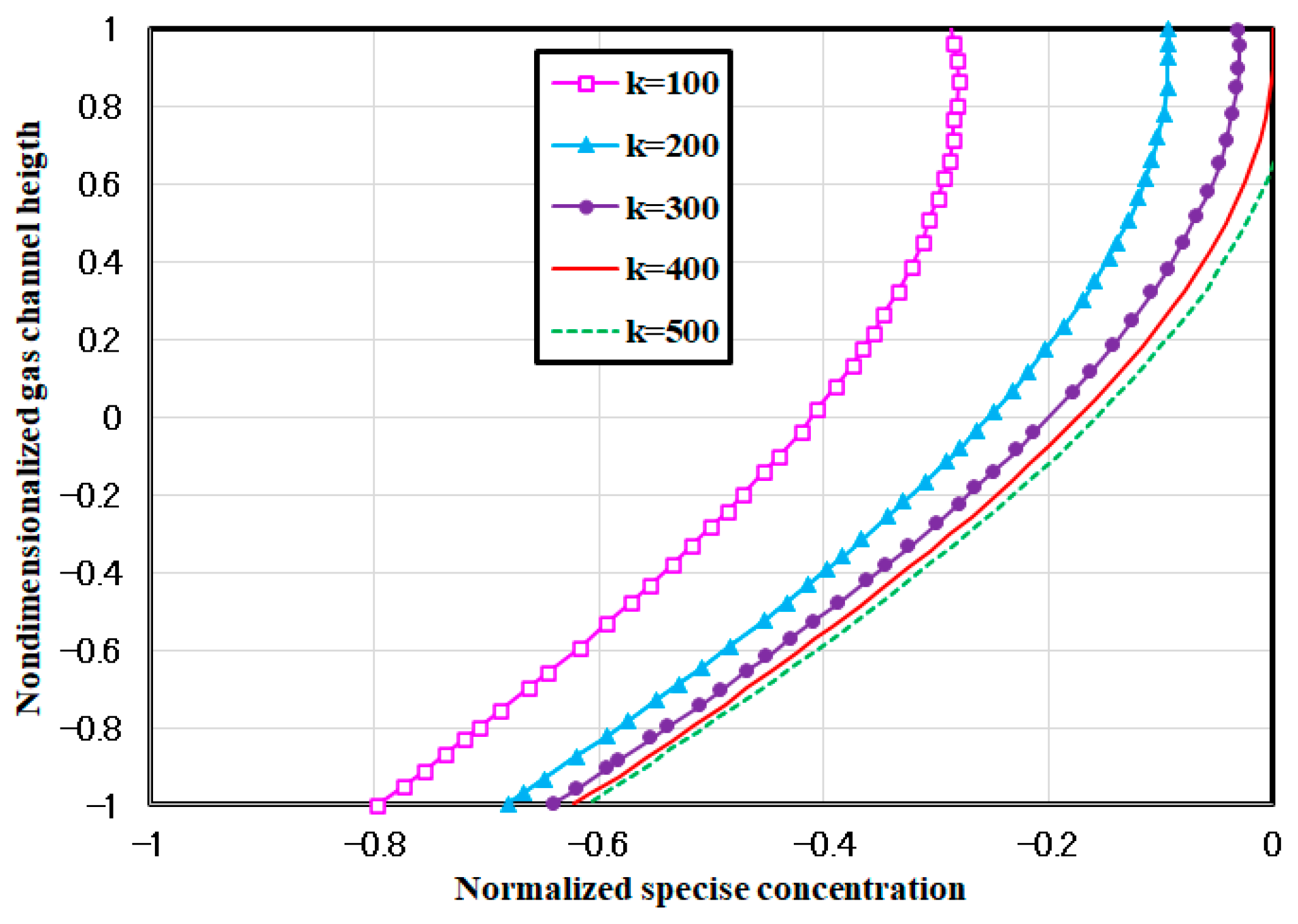
2.3.4. The Effect of Parameter k Changes on the Distribution of Species in the Channel

Along with the rapid decrease in the concentration of species at the beginning of the channel, the concentration of species along the channel decreases with a gentle slope, which is a function of the k parameter. Since parameter k is defined as $\frac{3}{2}Re\cdot Sc$ (called the Peclet number in mass transfer), this parameter represents the ratio of the axial velocity along the channel to the diffusion rate of the species ($\frac{3}{2}\cdot \frac{u\cdot x}{D}$). It is inferred from the k parameter that the higher the value of this parameter, the lower the diffusion rate of the species (and the concentration gradient) along the channel. In other words, the diffusion rate will decrease, and in contrast, by reducing this parameter, the rate of penetration of species will increase. Considering that, in this section, the geometric dimensions of the problem have become dimensionless with half of the channel height, for a fuel cell with a channel length of 50 mm and a channel height of 1 mm, the value of the dimensionless length of the channel or parameter x will be equal to 100. According to these values, the amount of the Reynolds number is considered constant and equal to Re = 200. The Schmidt number for the mixture of O₂, N₂, and H₂O gases, as well as for H₂ and H₂O, is equal to 0.56 to 0.74 [35,38]. According to the previous information, the value of the k parameter in the fuel cell varies between 160 and 260. Figure 6 represents the changes in the mass fraction of the species along the middle of the fuel cell channel for different values of the k parameter.

Figure 7 shows the changes in the mass fraction of species at the height of the gas channel (y direction) for different parameters k at x = 20. As k increases, the concentration of species inside the channel increases (consumption of species decreases).

2.4. Solving the Energy Equation to Find the Temperature Distribution

For finding the temperature distribution, the u₀ term of the velocity profile is substituted in the energy equation (Equation (37)). It should be noted that the procedure of solving the energy equation in the gas channel, taking into account the diffusion phenomenon, is similar to solving the species equation in the channel, which has been explained in the previous section. The boundary conditions will be slightly different, which will be explained later.

$$\begin{array}{c}u\approx u_0=\frac{3}{2}\left(1-y^2\right)\\ u\frac{\partial T}{\partial x}+v\frac{\partial T}{\partial y}=\frac{1}{Re.Pr}\frac{{\partial }^{2}T}{\partial y^2}\end{array}$$

(37)

By assuming $\frac{3}{2}Re.Pr=k^{\prime }$ and assuming the velocity of diffusion from the bottom of the channel as—_s. We will have Equations (38) and (39), respectively:

$$\frac{3}{2}Re.Pr.\left(1-y^2\right)\frac{\partial T}{\partial x}-Re.Pr{.v}_s.\frac{\partial T}{\partial y}=\frac{{\partial }^{2}T}{\partial y^2}$$

(38)

$$k^{\prime }.\left(1-y^2\right)\frac{\partial T}{\partial x}-Re.Pr{.v}_s.\frac{\partial T}{\partial y}=\frac{{\partial }^{2}T}{\partial y^2}$$

(39)

2.4.1. Dimensioning the Energy Equation and Applying Boundary Conditions

To nondimensionalize the temperature, the following relation is used:

$$T=\frac{\overline{T}-T_{\infty }}{T_{add}-T_{\infty }}$$

The temperature boundary condition in the gas channel related to the polymer fuel cell is a constant temperature, and it is assumed that the inlet gas flow has a temperature equal to the operating temperature of the fuel cell (in this case, it is 353 K). The temperature of the upper surface of the channel is equal to the temperature of the cooling fluid because it is subjected to cooling by the cooling fluid. For better performance of the cell, the maintenance of the temperature of the cell around the operating temperature (353 K) is attempted. Due to the chemical reactions, the temperature of the fuel cell in the areas where the reaction takes place is about 6 K higher than the operating temperature. By using the finite volume method of computational fluid dynamics, the temperature distribution profile at the bottom of the channel is shown in Figure 8, referring to the results of Figure 8 with a very good approximation and considering that the average temperature at the bottom of the channel is equal to 356 K.

The temperature of the top of the gas channel is equal to 353 K, and the temperature of the fluid flow ${\overline{T}}_{add}$ is equal to 353 K, and the temperature is equal to the temperature of the bottom of the gas channel. This temperature is slightly higher than in other parts of the channel (around 3 Kelvin) because of the proximity of the channel bottom to the reaction area. Therefore, after nondimensionalization, the boundary conditions will be as follows:

$$\mathrm{Boundary} \mathrm{condition}: T\left(0,y\right)=0, T\left(x,\frac{1}{2}\right)=0, T\left(x,-\frac{1}{2}\right)=1.$$

2.4.2. Applying Perturbation Parameters and Solving Energy

The perturbation parameter is as $Re·Pr·v_s=\gamma .$ Therefore, the equations and temperature profile will be as follows, and Equations (40)–(43) are extracted:

$$T=T_0+\gamma T_1+{\gamma }^2{T}_2+\dots$$

$$\begin{array}{c}{k}^{\prime }.\left(1-y^2\right)\frac{\partial T}{\partial x}-\gamma .\frac{\partial T}{\partial y}=\frac{{\partial }^{2}T}{\partial y^2}\hfill \\ k^{\prime }.\left(1-y^2\right)\frac{\partial }{\partial x}\left(T_0+\gamma T_1+{\gamma }^2{T}_2+\dots \right)-\gamma \frac{\partial }{\partial y}\left(T_0+\gamma T_1+{\gamma }^2{T}_2+\dots \right)=\frac{{\partial }^2}{\partial y^2}\left(T_0+\gamma T_1+{\gamma }^2{T}_2+\dots \right)\hfill \end{array}$$

$$\begin{array}{c}{\gamma }^0:k^{\prime }\left(1-y^2\right)\frac{\partial T_0}{\partial x}=\frac{{\partial }^2{T}_0}{\partial y^2}\hfill \\ BC:T_0 (0, y)=0, T_0\left(x,\frac{1}{2}\right)=0 T_0\left(x,-\frac{1}{2}\right)=1\hfill \end{array}$$

(40)

$$\begin{array}{c}{\gamma }^1: k^{\prime }.\left(1-y^2\right)\frac{\partial T_1}{\partial x}=\frac{{\partial }^2{T}_1}{\partial y^2}+\frac{\partial T_0}{\partial y}\hfill \\ BC:T_1 (0, y)=0, T_1\left(x,\frac{1}{2}\right)=0 T_1\left(x,-\frac{1}{2}\right)=0\hfill \end{array}$$

(41)

$$\begin{array}{c}{\gamma }^2: k^{\prime }.\left(1-y^2\right)\frac{\partial T_2}{\partial x}=\frac{{\partial }^2{T}_2}{\partial y^2}+\frac{\partial T_1}{\partial y}\hfill \\ BC:T_2 (0, y)=0, T_2\left(x,\frac{1}{2}\right)=0 T_2\left(x,-\frac{1}{2}\right)=0\hfill \end{array}$$

(42)

For reducing the effect of the y² term, the method of solving the species equation is also used here, and the equations will be solved to find the temperature distribution up to the first-order accuracy for γ. After solving the answers related to T₀ and T₁, they will be combined, and the final answer will be obtained. The equations obtained from the previous step are powers of γ⁰ and γ¹. These values of δ⁰ power base have been obtained. These equations (Equations (43)–(47)) are as follows:

• γ⁰:

  $$k^{\prime }\frac{\partial T_0}{\partial x}=\frac{{\partial }^2{T}_0}{\partial y^2}$$

  (43)

  $$BC:T_0 (0, y)=0, T_0\left(x,\frac{1}{2}\right)=0 T_0\left(x,-\frac{1}{2}\right)=1$$

For solving Equation (43), the method mentioned in solving the species equation is used. After solving, the answer for T₀ is as in Equation (44):

$$T_0(x,y)=-y+{\displaystyle \sum _{n=1}^{\infty }(}-\frac{2}{n^2{\pi }^2}\cdot e^{\frac{-n^2{\pi }^2}{k^{\prime }}x}(n\pi \cos (n\pi )-\sin (n\pi )))\cdot \sin (n\pi y)$$

(44)

For the T₁, we have Equation (45) and perform the same method.

• γ¹:

  $$k^{\prime }.\frac{\partial T_1}{\partial x}=\frac{{\partial }^2{T}_1}{\partial y^2}+\frac{\partial T_0}{\partial y}$$

  (45)

  $$\mathrm{BC}: T0 (0, y)=0, T_0\left(x,\frac{1}{2}\right)=0 \to T_1\left(x,-\frac{1}{2}\right)=0$$

After solving, the answer for T₁ will be as in Equation (46):

$$T_1(x,y)=-\frac{x}{k^{\prime }}-{\displaystyle \sum _{n=1}^{\infty }\left(\frac{x{e}^{-\frac{n^2{\pi }^2}{k^{\prime }}x}}{k^{\prime }}\cos (n\pi )\right)}\cos n\pi y$$

(46)

Therefore, the general solution of the heat distribution equation in the gas channel, the second-order precision base of the perturbation parameter, after solving Equations (44) and (46) using the method presented in Appendix A and by solving the equations of the differential with partial derivatives, are presented by the method of eigenfunction expansion. After solving the equations, the solutions are combined and provide the temperature distribution in the gas channel as Equation (47):

$$T=T_0+\gamma T_1+{\gamma }^2{T}_2$$

$$T(x,y)=-y+{\displaystyle \sum _{n=1}^{\infty }\frac{-2e^{-\frac{n^2{\pi }^2}{k^{\prime }}x}\left(n\pi \cos (n\pi )-\sin (n\pi )\right)\sin n\pi y}{{(n\pi )}^2}}+\gamma \left(-\frac{x}{k^{\prime }}-{\displaystyle \sum _{n=1}^{\infty }\left(\frac{x{e}^{-\frac{n^2{\pi }^2}{k^{\prime }}x}}{k^{\prime }}\cos (n\pi y)\right)}\right)+{\gamma }^2\left(0\right)$$

(47)

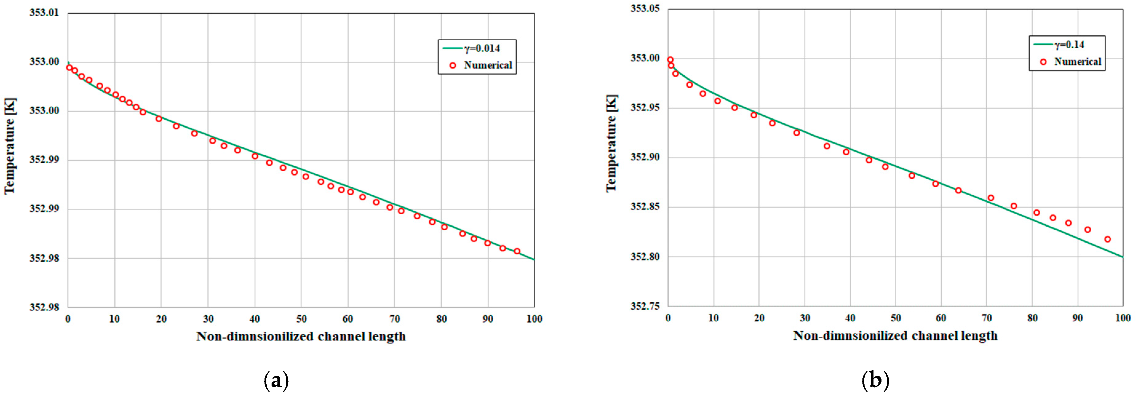
2.4.3. Comparison of Numerical and Analytical Results

Figure 9 compares the analytical and numerical results obtained from the numerical method of computational fluid dynamics based on finite volume for the changes in the temperature distribution of the reactant flow along the center line of the gas channel for different diffusion velocities, which indicates that the numerical and analytical results are in very good agreement.

Table 3. Error comparison of the numerical and analytical results for energy equation.

	The Value of the Perturbation Parameter	Error $\left(\frac{\mathit{n}\mathit{u}\mathit{m}\mathit{e}\mathit{r}\mathit{i}\mathit{c}\mathit{a}\mathit{l}-\mathit{a}\mathit{n}\mathit{a}\mathit{l}\mathit{y}\mathit{t}\mathit{i}\mathit{c}\mathit{a}\mathit{l}}{\mathit{n}\mathit{u}\mathit{m}\mathit{e}\mathit{r}\mathit{i}\mathit{c}\mathit{a}\mathit{l}}\times \mathbf{100}\right)$
1	γ = 0.014	0.03
2	γ = 0.14	0.45

presents the amount of error between the numerical and analytical results. The numerical and analytical results have been compared for two perturbation parameters that are a function of diffusion velocity.

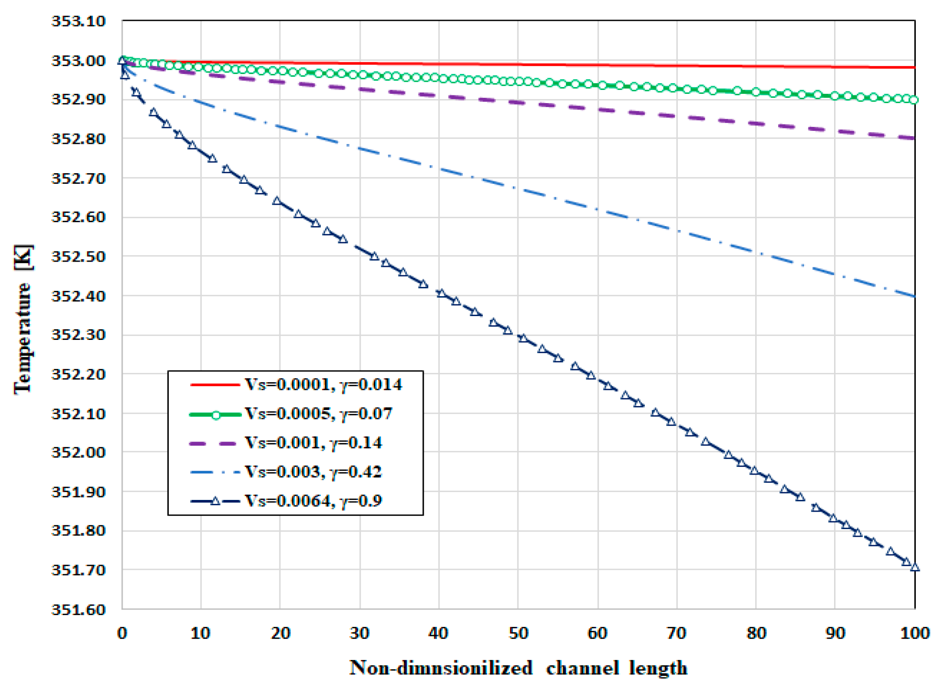
2.4.4. The Effect of Species Diffusion Rate on Temperature Distribution

Figure 10 shows the temperature distribution along the channel centerline for different species diffusion rates in the gas channel. The temperature profile shows that with the rate of diffusion of species caused by the increase in porosity, the amount of temperature gradient increases in the longitudinal direction. Also, the temperature of the gas at the outlet of the channel decreases with the increase in the diffusion rate of the species. The justification for this is that, with the increase in the diffusion rate of species from the bottom of the gas channel (in the direction perpendicular to the bottom of the channel), the convective heat transfer power caused by the increase in vertical speed has increased. As a result, with the increase in velocity, the temperature in the middle of the channel will decrease along the channel. The higher the perturbation parameter, which is a function of the diffusion velocity, increases, the greater the temperature drop will be at the end of the channel.

Figure 11 shows the vertical temperature distribution (from the top to the bottom of the channel) in the gas channel for different diffusion velocities along the same length of the channel. The vertical temperature distribution along the same length has been investigated at the beginning, middle, and end of the channel, which is indicated as x = 10, x = 50, and x = 90, respectively, in Figure 11a–c. As can be seen, the vertical temperature distribution in the same length in the gas channel is moving to the end of the channel, and the temperature profile shows a more linear behavior. The reason for this mathematically is that as the length of the channel increases, the influence of the term $-\frac{x}{k^{\prime }}$ is increased compared to the exponential term. Therefore, the temperature distribution function in the exit regions will appear more linear. The physical reason for this will also be related to the increase in the convective heat transfer rate. As previously discussed in Figure 10, because of the distribution of temperature along the channel caused by the increase in convective heat transfer in the flow direction and the channel, the middle points of the channel will have a temperature difference in the vertical direction, which is much more severe at the endpoints of the channel. By looking at the profiles above, it can be seen that as the rate of diffusion and, consequently, the perturbation parameter increases, the maximum temperatures at the bottom and top of the channel will also decrease. In other words, the maximum temperature in the channel is also reduced, which is due to the increase in the convective heat transfer power in the vertical and downward directions. Mathematically, this is also logical because, with the increase in the perturbation parameter, the contribution of the second term of the equation, which has a negative sign, also increases, which will decrease the temperature profile with the increase in velocity.

3. Conclusions

The present study is focused on developing an analytical and mathematics-based model to predict the transport phenomena and output performance of the PEMFC in the different penetration (diffusion) velocities from the bottom of the flow channels. As well, a 3D CFD model based on the finite volume is also developed to validate the analytical results. The penetration velocity mainly depends on the porosity of the GDLs, and also, it is the function of the operating pressure. In the present study, the perturbation method is applied to solve the governing equation of fluid flow within the PEMFC flow channel. After solving the governing equation and equations using the perturbation method, the following results are achieved:

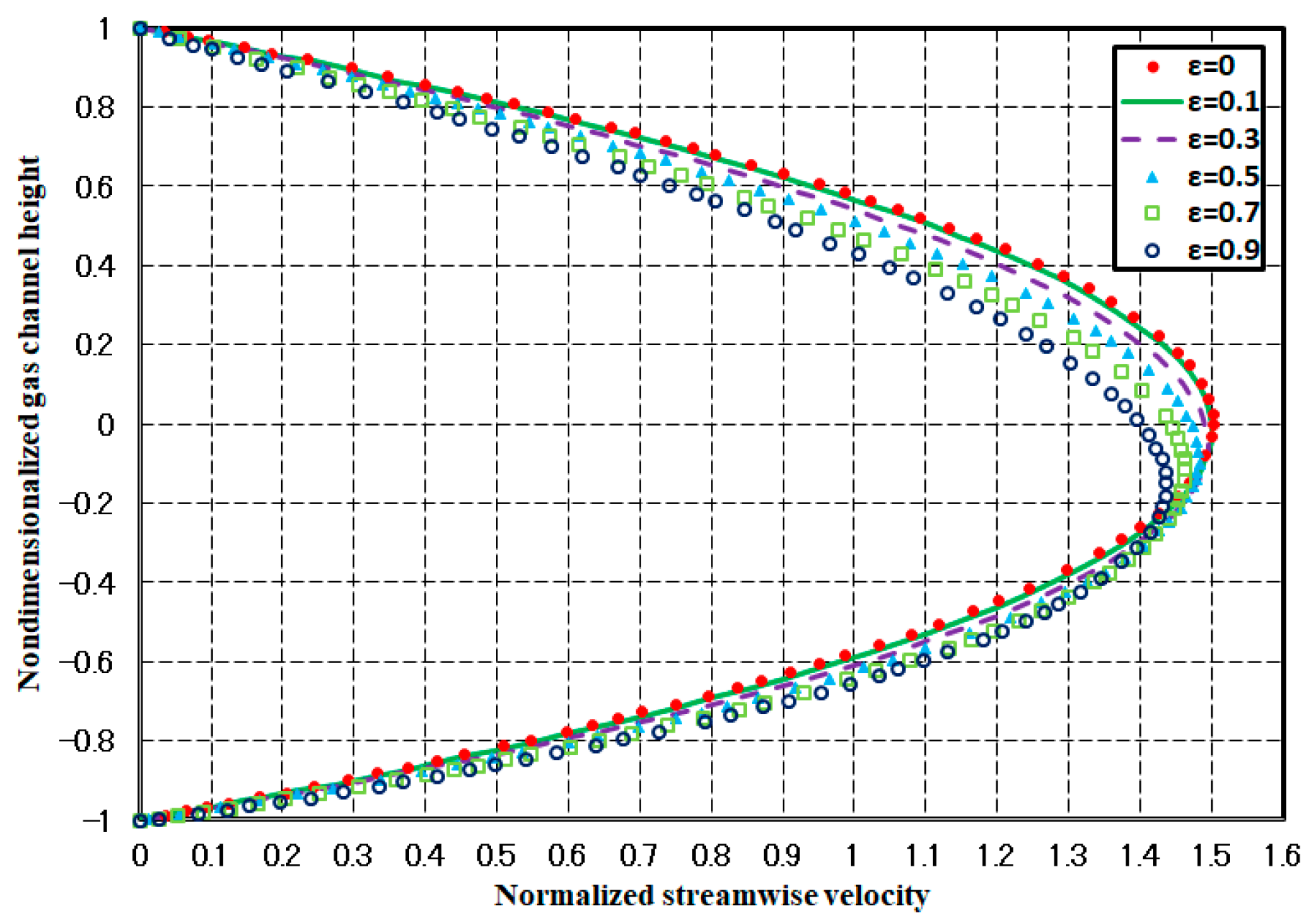
• The axial velocity profile maximum section tends into the bottom of the channel, and also, the maximum value of the axial velocity decreases while the perturbation parameter (penetration velocity) increases. For the higher values of the perturbation parameter, tending the maximum part of the velocity profile into the bottom of the channel conducts the reactant species much better than lower values and reduces the concentration loss of the reactant. This fact is also obvious in the numerical results.
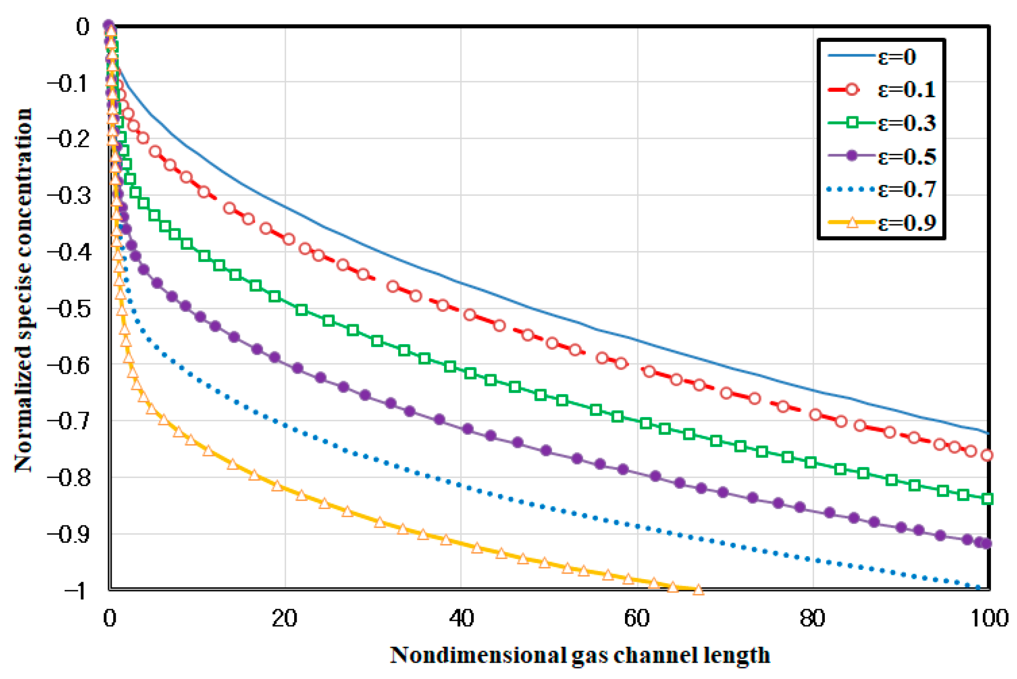
• In the solution of the species equation, the different perturbation parameter from the momentum equation is chosen. The perturbation parameter is the multiplication of the penetration velocity, Reynolds number, and Schmidt number.
• The results indicate that by increasing the perturbation parameter in the species equation, the reactant concentration gradient is enhanced in the direction of the flow in the gas channel. This fact is due to increasing the penetration of the reactants into the GDLs. For the higher values of the perturbation parameter from 0.7, there is a big gradient in the channel, which leads to the lake of the species at the end of the gas channel. This fact results in higher ohmic loss and decreases the performance of the fuel cell.
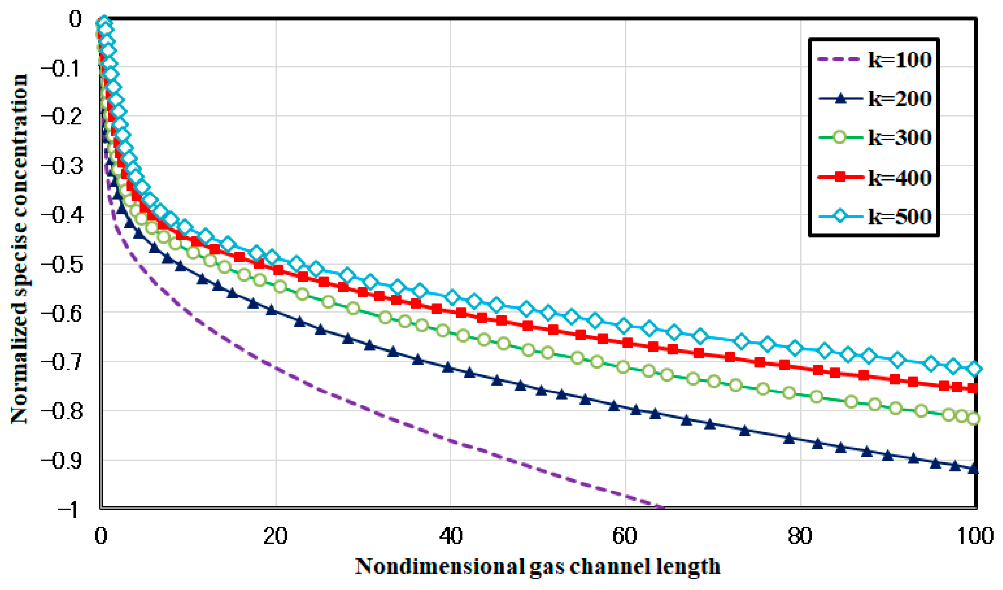
• The achieved results of the species profile in the gas channel for the different magnitudes of the Peclete number indicate that for the lower magnitudes of the k than 200, the species gradient is enhanced, and as a result, the concentration loss takes place at the exit region of the channel.
• Also, the Peclete number affects the normal profile of the species distribution of the species in the gas channel. For smaller k, the profile tends backward because of the enhancement of the species transferring from the channel. In the higher Peclete numbers, the reactant, because of the higher convection magnitude, has lower values of diffusion. In other words, increasing the convection magnitude affects the diffusion rate reversely.
• In the energy equation, the multiplication of the penetration rate, Reynolds number, and Prandtle number is chosen as the perturbation parameter. Increasing the perturbation parameter reduces the convective heat transfer rate, and as a result, the temperature gradient is increased in the flow direction.
• Increasing the perturbation parameter from smaller values to higher values converts the nonlinear normal temperature profile to the linear one. It takes place because by increment of the perturbation parameter, in Equation (62), the impact of the linear term would be significant. Also, the physical reason is that augmentation of the perturbation parameter causes a powerful diffusion and convection heat transfer in the normal direction of the flow.
• For each analytical procedure, the results have been compared to the numerical simulation results. The numerical results also show the same magnitude and trend for each curve, which certifies the analytical model.
• As is indicated, compared to the 3D numerical results, the analytical results can provide more accurate and reliable results in less time than numerical simulation. In other words, the analytical model can predict the effect of the geometrical configuration on the fuel cell transport phenomena and performance. However, the numerical model is a general model that, in addition, can take into account the electrochemical reaction and the effect of these reactions on the cell performance.

As a suggestion for future work, the solution of the same equations can be performed by assuming a nonlinear and nonconstant species flux at the bottom of the channel as the boundary condition. Also, this method will be used for the solution of the Navier–Stokes equation in the reaction area.

References

1. Ashrafi, H.; Pourmahmoud, N.; Mirzaee, I.; Ahmadi, N. Performance improvement of proton-exchange membrane fuel cells through different gas injection channel geometries. Int. J. Energy Res. 2022, 46, 8781–8792. [Google Scholar] [CrossRef]
2. Hossein, S.; Ahmadi, N.; Jabbary, A. Effects of applying brand-new designs on the performance of PEM fuel cell and water flooding phenomena. Iran. J. Chem. Chem. Eng. 2022, 41. [Google Scholar] [CrossRef]
3. Ganguly, D.; Ramanujam, K.; Sundara, R. Low-Temperature Synthesized Pt3Fe Alloy Nanoparticles on Etched Carbon Nanotubes Catalyst Support Using Oxygen-Deficient Fe2O3 as a Catalytic Center for PEMFC Applications. ACS Sustain. Chem. Eng. 2023, 11, 3334–3345. [Google Scholar] [CrossRef]
4. Ahmadi, N.; Ahmadpour, V.; Rezazadeh, S. Numerical investigation of species distribution and the anode transfer coefficient effect on the proton exchange membrane fuel cell (PEMFC) performance. Heat Transf. Res. 2015, 46, 881–901. [Google Scholar] [CrossRef]
5. Oksuztepe, E.; Bayrak, Z.U.; Kaya, U. Effect of flight level to maximum power utilization for PEMFC/supercapacitor hybrid uav with switched reluctance motor thruster. Int. J. Hydrogen Energy 2023, 48, 11003–11016. [Google Scholar] [CrossRef]
6. Hossein, S.; Ahmadi, N.; Mirzaee, I.; Abbasalizade, M. The Study of Cylindrical Polymer Fuel Cell’s Performance and the Investigation of Gradual Geometry Changes’ Effect on Its Performance. Period. Polytech. Chem. Eng. 2019, 63, 513–526. [Google Scholar]
7. Sun, Y.; Mao, L.; He, K.; Liu, Z.; Lu, S. Imaging PEMFC performance heterogeneity by sensing external magnetic field. Cell Rep. Phys. Sci. 2022, 3, 101083. [Google Scholar] [CrossRef]
8. Jarry, T.; Jaafar, A.; Turpin, C.; Lacressonniere, F.; Bru, E.; Rallieres, O.; Scohy, M. Impact of high frequency current ripples on the degradation of high-temperature PEM fuel cells (HT-PEMFC). Int. J. Hydrogen Energy 2023, 48, 20734–20742. [Google Scholar] [CrossRef]
9. Ahmadi, N.; Pourmahmoud, N.; Mirzaee, I.; Rezazadeh, S. Three-dimensional computational fluid dynamic study on performance of polymer exchange membrane fuel cell (PEMFC) in different cell potential. Iran. J. Sci. Technol. Trans. Mech. Eng. 2012, 36, 129. [Google Scholar]
10. Seo, B.G.; Koo, J.; Jeong, H.J.; Park, H.W.; Kim, N.I.; Shim, J.H. Performance Enhancement of Polymer Electrolyte Membrane Fuel Cells with Cerium Oxide Interlayers Prepared by Aerosol-Assisted Chemical Vapor Deposition. ACS Sustain. Chem. Eng. 2023, 11, 10776–10784. [Google Scholar] [CrossRef]
11. Liu, W.; Sun, B.; Lai, Y.; Yu, Z.; Xie, N. Performance improvement of an integrated system with high-temperature PEMFC, Kalina cycle and concentrating photovoltaic (CPV) for low temperature heat recovery. Appl. Therm. Eng. 2023, 220, 119659. [Google Scholar] [CrossRef]
12. Zhu, W.; Han, J.; Ge, Y.; Yang, J.; Liang, W. Performance analysis and multi-objective optimization of a poly-generation system based on PEMFC, DCMD and heat pump. Desalination 2023, 555, 116542. [Google Scholar] [CrossRef]
13. Chu, D.; Jiang, R. Performance of polymer electrolyte membrane fuel cell (PEMFC) stacks: Part I. Evaluation and simulation of an air-breathing PEMFC stack. J. Power Sources 1999, 83, 128–133. [Google Scholar] [CrossRef]
14. Moore, J.M.; Adcock, P.L.; Lakeman, J.; Mepsted, G.O. The effects of battlefield contaminants on PEMFC performance. J. Power Sources 2000, 85, 254–260. [Google Scholar] [CrossRef]
15. Hamelin, J.; Agbossou, K.; Laperrière, A.; Laurencelle, F.; Bose, T. Dynamic behavior of a PEM fuel cell stack for stationary applications. Int. J. Hydrogen Energy 2001, 26, 625–629. [Google Scholar] [CrossRef]
16. Mann, R.F.; Amphlett, J.C.; Hooper, M.A.I.; Jensen, H.M.; Peppley, B.A.; Roberge, P.R. Development and application of a generalised steady-state electrochemical model for a PEM fuel cell. J. Power Sources 2000, 86, 173–180. [Google Scholar] [CrossRef]
17. Li, Z.; Bai, F.; He, P.; Zhang, Z.; Tao, W.-Q. Three-dimensional performance simulation of PEMFC of metal foam flow plate reconstructed with improved full morphology. Int. J. Hydrogen Energy 2023, 48, 27778–27789. [Google Scholar] [CrossRef]
18. Dong, Z.; Qin, Y.; Zheng, J.; Guo, Q. Numerical investigation of novel block flow channel on mass transport characteristics and performance of PEMFC. Int. J. Hydrogen Energy 2023, 48, 26356–26374. [Google Scholar] [CrossRef]
19. Sun, Y.; Mao, L.; Wang, H.; Liu, Z.; Lu, S. Simulation study on magnetic field distribution of PEMFC. Int. J. Hydrogen Energy 2022, 47, 33439–33452. [Google Scholar] [CrossRef]
20. Shang, K.; Han, C.; Jiang, T.; Chen, Z. Numerical study of PEMFC heat and mass transfer characteristics based on roughness interface thermal resistance model. Int. J. Hydrogen Energy 2023, 48, 7460–7475. [Google Scholar] [CrossRef]
21. Xu, C.; Wang, H.; Cheng, T. Wave-shaped flow channel design and optimization of PEMFCs with a groove in the gas diffusion layer. Int. J. Hydrogen Energy 2023, 48, 4418–4429. [Google Scholar] [CrossRef]
22. Duan, F.; Song, F.; Chen, S.; Khayatnezhad, M.; Ghadimi, N. Model parameters identification of the PEMFCs using an improved design of Crow Search Algorithm. Int. J. Hydrogen Energy 2022, 47, 33839–33849. [Google Scholar] [CrossRef]
23. Xia, L.; Xu, Q.; He, Q.; Ni, M.; Seng, M. Numerical study of high temperature proton exchange membrane fuel cell (HT-PEMFC) with a focus on rib design. Int. J. Hydrogen Energy 2021, 46, 21098–21111. [Google Scholar] [CrossRef]
24. Liu, S.; Chen, T.; Zhang, C.; Xie, Y. Study on the performance of proton exchange membrane fuel cell (PEMFC) with dead-ended anode in gravity environment. Appl. Energy 2020, 261, 114454. [Google Scholar] [CrossRef]
25. Zhang, G.; Jiao, K. Three-dimensional multi-phase simulation of PEMFC at high current density utilizing Eulerian-Eulerian model and two-fluid model. Energy Convers. Manag. 2018, 176, 409–421. [Google Scholar] [CrossRef]
26. Mahdavi, A.; Ranjbar, A.A.; Gorji, M.; Rahimi-Esbo, M. Numerical simulation based design for an innovative PEMFC cooling flow field with metallic bipolar plates. Appl. Energy 2018, 228, 656–666. [Google Scholar] [CrossRef]
27. Yin, Y.; Wang, X.; Shangguan, X.; Zhang, J.; Qin, Y. Numerical investigation on the characteristics of mass transport and performance of PEMFC with baffle plates installed in the flow channel. Int. J. Hydrogen Energy 2018, 43, 8048–8062. [Google Scholar] [CrossRef]
28. Zhao, J.; Li, S.; Tu, Z. Development of practical empirically and statistically-based equations for predicting the temperature characteristics of PEMFC applied in the CCHP system. Int. J. Hydrogen Energy 2023, in press. [CrossRef]
29. Chu, T.; Tang, Q.; Wang, Q.; Wang, Y.; Du, H.; Guo, Y.; Li, B.; Yang, D.; Ming, P.; Zhang, C. Experimental study on the effect of flow channel parameters on the durability of PEMFC stack and analysis of hydrogen crossover mechanism. Energy 2023, 264, 126286. [Google Scholar] [CrossRef]
30. Tsai, C.; Chen, F.; Ruo, A.; Chang, M.-H.; Chu, H.-S.; Soong, C.; Yan, W.; Cheng, C. An analytical solution for transport of oxygen in cathode gas diffusion layer of PEMFC. J. Power Sources 2006, 160, 50–56. [Google Scholar] [CrossRef]
31. Neyerlin, K.C.; Gu, W.; Jorne, J.; Clark, A.; Hubert, A. Gasteiger. Cathode catalyst utilization for the ORR in a PEMFC: Analytical model and experimental validation. J. Electrochem. Soc. 2007, 154, B279. [Google Scholar] [CrossRef]
32. Haji, S. Analytical modeling of PEM fuel cell i–V curve. Renew. Energy 2011, 36, 451–458. [Google Scholar] [CrossRef]
33. Ahmadi, N.; Dadvand, A.; Mirzaei, I.; Rezazadeh, S. Modeling of polymer electrolyte membrane fuel cell with circular and elliptical cross-section gas channels: A novel procedure. Int. J. Energy Res. 2018, 42, 2805–2822. [Google Scholar] [CrossRef]
34. Liu, S.; Chen, T.; Xie, Y. A two-dimensional analytical model of PEMFC with dead-ended anode. Int. J. Green Energy 2020, 17, 255–273. [Google Scholar] [CrossRef]
35. Ahmadi, N.; Kõrgesaar, M. Analytical approach to investigate the effect of gas channel draft angle on the performance of PEMFC and species distribution. Int. J. Heat Mass Transf. 2020, 152, 119529. [Google Scholar] [CrossRef]
36. Kulikovsky, A.A. Quasi-3D modeling of water transport in polymer electrolyte fuel cells. J. Electrochem. Soc. 2003, 150, A1432. [Google Scholar] [CrossRef]
37. Nayfeh, A.H. Introduction to Perturbation Techniques; John Wiley & Sons: Hoboken, NJ, USA, 2011. [Google Scholar]
38. Sung, Y. An approximate analytical solution to channel flow in a fuel cell with a draft angle. J. Power Sources 2006, 159, 1051–1060. [Google Scholar] [CrossRef]
Figure 1. Schematic of solution domain and velocity components inside the gas channel.
Mathematics 11 04094 g001
Figure 2. Comparison of analytical and numerical results for different perturbation parameters ((a) for ε = 0 and (b) for ε = 0.5).
Mathematics 11 04094 g002
Figure 3. Comparison of velocity distribution in fuel cell gas channel for different perturbation parameters.
Mathematics 11 04094 g003
Figure 4. Comparison of analytical and numerical results for different perturbation parameters ((a) for ε = 0 and (b) for ε = 0.5).
Mathematics 11 04094 g004
Figure 5. Distribution of species concentration along the channel (A = 10, k = 200, and y = −1/2) for different perturbation parameters.
Mathematics 11 04094 g005
Figure 6. Distribution of the species along the middle of the fuel cell channel for different values of the k parameter.
Mathematics 11 04094 g006
Figure 7. Distribution of the species for different parameters k at x = 20.
Mathematics 11 04094 g007
Figure 8. Mean temperature distribution extracted from numerical results.
Mathematics 11 04094 g008
Figure 9. Comparison of analytical and numerical results for different disturbance parameters ((a) for γ = 0.014 and (b) for γ = 0.14).
Mathematics 11 04094 g009
Figure 10. Comparison of temperature distribution along the centerline of the gas channel for different channel diffusion velocities.
Mathematics 11 04094 g010
Figure 11. Comparison of temperature distribution at y direction in the same length: (a) for (X = 10), (b) for (X = 50), and (c) for (X = 90).
Mathematics 11 04094 g011