Broad Learning Model with a Dual Feature Extraction Strategy for Classification

Abstract

The broad learning system (BLS) is a brief, flat neural network structure that has shown effectiveness in various classification tasks. However, original input data with high dimensionality often contain superfluous and correlated information affecting recognition performance. Moreover, the large number of randomly mapped feature nodes and enhancement nodes may also cause a risk of redundant information that interferes with the conciseness and performance of the broad learning paradigm. To address the above-mentioned issues, we aim to introduce a broad learning model with a dual feature extraction strategy (BLM_DFE). In particular, kernel principal component analysis (KPCA) is applied to process the original input data before extracting effective low-dimensional features for the broad learning model. Afterwards, we perform KPCA again to simplify the feature nodes and enhancement nodes in the broad learning architecture to obtain more compact nodes for classification. As a result, the proposed model has a more straightforward structure with fewer nodes and retains superior recognition performance. Extensive experiments on diverse datasets and comparisons with various popular classification approaches are investigated and evaluated to support the effectiveness of the proposed model (e.g., achieving the best result of 77.28%, compared with 61.44% achieved with the standard BLS, on the GT database).

1. Introduction

Many intelligent methods, e.g., nearest-neighbor classifiers, support vector machine, and neural networks, have been developed and implemented for various classification applications [1,2]. Among them, the neural network is one of the most popular and attractive methods at present. For instance, some deep neural networks have shown remarkable performance and obtained breakthroughs in many areas, including pattern recognition and image processing tasks, in recent years [3]. The essential ideas of these typical, deep neural networks aim to deepen the layers of neural networks and then obtain more high-level features from input data [4]. However, due to a large number of layers and complicated structure with huge hyper-parameters, the training process is quite long and tedious, which may affect the deployment and application of real-world classification tasks. In addition, deep networks usually require the support of powerful computing resources that are calculation-expensive at present [5]. Moreover, the complicated architecture of these models brings many difficulties in analyzing them theoretically. Thus, the flat neural network with a brief structure and fewer parameters is a flexible and competitive model [6]. It can achieve reasonable classification results without a complicated structure and a long training process.

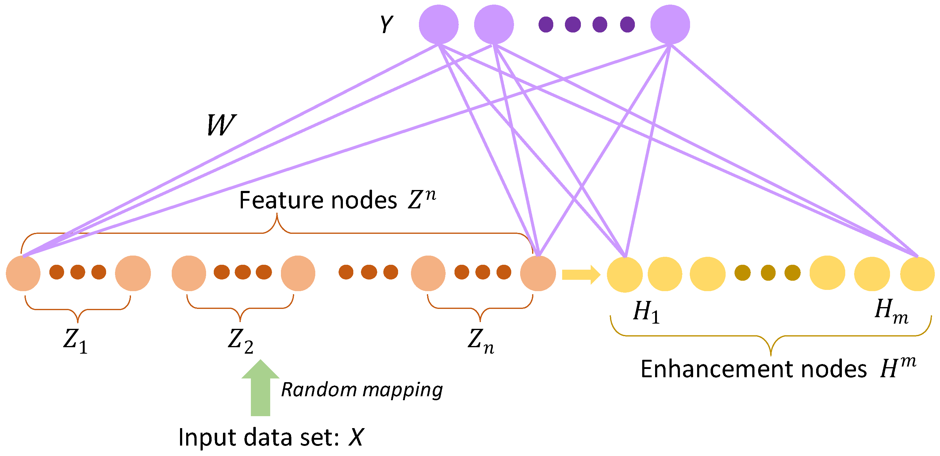
Many researchers have recently developed and investigated the broad learning system (BLS), an attractive, flat neural network [6]. It is designed and implemented according to the random vector functional-link neural network (RVFLNN), a fast model that provides the generalization ability of functional approximation [7]. The BLS not only inherits the advantages of the RVFLNN but also obtains remarkable performance. The principles of basic broad learning (BL) are quite concise. Specifically, the input training data are randomly mapped to produce the corresponding feature nodes at first. Then, the generated mapped feature nodes are further treated and mapped with random weights to generate enhancement nodes. In this way, both feature nodes and enhancement nodes are utilized to compute the output results based on ridge regression approximation. The learned weights obtained using ridge regression approximation can be applied to the test data to generate the corresponding predicted results [6].

The BLS is effective and has shown brilliant results in diverse classification and pattern recognition studies. Many researchers have developed and implemented this model and made many meaningful achievements [8,9,10,11,12,13]. For instance, Feng et al. implemented and integrated a fuzzy system into the basic BLS to replace original feature nodes with a group of Takagi–Sugeno fuzzy subsystems [14]. Their experimental results show that their proposed model achieves suitable performance compared with other models. The authors in [15] aimed to modify and replace the ridge regression approximation of standard BL with the regularized discriminative approach to generate more effective learned weights for image classification and then demonstrated the model’s outstanding classification capability. Researchers ameliorated the BLS structure, obtaining recurrent-BLS and Gated-BLS, for text classification and received the desired results in training time and accuracy [16]. Yang et al. indicated that feature nodes and enhancement nodes may contain inefficient and redundant features. They performed a series of autoencoders on the BLS to acquire more effective features for various classification applications [17]. Other researchers also attempted to combine a deep model, such as Convolutional Neural Network (CNN), with the BLS for classification and showed that their model is flexible in many applications [18]. Chen et al. adopted a similar strategy to implement a CNN-based broad learning model that extracts valuable features of facial emotional images before classifying emotions [19]. Many scholars have investigated the BLS in diverse applications. Sheng et al. developed a visual-based assessment system to evaluate a soccer game according to the BLS, which was effective in assessing trainees’ performance [20]. In Ref. [21], the authors implemented a discriminant manifold BLS method to classify hyperspectral images and effectively enhanced the recognition accuracy with limited training samples. In Ref. [22], the researchers proposed a competitive BLS method for COVID-19 detection based on CT scans or chest X-ray images. In addition, Zhou et al. also investigated the BLS in the healthcare area and developed a semi-supervised BLS within transfer learning for EEG signal recognition [23]. Other researchers implemented the BLS with decomposition algorithms for AQI forecasting and obtained ideal results [24]. Zhao et al. processed input signals with principal component analysis (PCA) to generate valuable features and employed it with the BLS for fault diagnosis in a rotor system. Their results indicate that the PCA method can achieve dimension reduction of the input data as well as the extraction of valid features, where the BLS can acquire accurate fault diagnosis results efficiently [25].

Although the BLS has been studied, upgraded, and applied in many aspects, it still has some deficiencies that need to be mitigated. For instance, traditional input data for the broad learning structure may contain high correlation and redundancy that can interfere with the recognition results. This issue is also mentioned and discussed in [25]. In addition, Chen et al. mentioned that the broad learning architecture may have redundant information that can be simplified in terms of the feature nodes and enhancement nodes [6]. A similar view is also reported in [17]. These above-mentioned limitations are caused by the redundancy or high correlation of the input or generated data. Many feature engineering approaches can alleviate these issues in the basic BLS. Thus, it is suitable to apply feature engineering methods for further processing to obtain more effective feature information and enhance the upgraded model’s performance.

Many techniques and algorithms have been developed and implemented for feature extraction from raw input data [26,27], which can obtain essential features and achieve dimensionality reduction. One of the widely used methods is PCA [28]. It can produce a series of orthogonal bases that acquire the directions of the maximum variance among input data, as well as the uncorrelated coefficients among new bases [29,30]. In this way, PCA explores a linear subspace with lower dimensionality compared with the original input feature space, where the new generated features retain the effective information for further analysis. Numerous studies have applied the PCA method for pattern recognition and classification and have shown favorable results. For example, Hargrove et al. implemented PCA to process the detected signals in pattern recognition-based myoelectric control and achieved remarkable results [31]. Howley et al. investigated PCA to process spectral data. They indicated that applying PCA can enhance classification performance with high-dimensional data [32].

Standard PCA is designed to perform linear dimensionality reduction. However, if the input data contain more complex structures that are difficult to represent in the linear subspace, basic PCA may perform poorly [33]. Fortunately, KPCA (kernel principal component analysis) is introduced and developed to process nonlinear dimension reduction as well as feature extraction [34]. This KPCA method has been widely utilized and verified in various applications. In Ref. [35], the authors applied KPCA to extract gait features and then evaluated it with support vector machine (SVM) to improve the recognition of gait patterns. Their results indicate that KPCA is effective for feature extraction, as well as dimensionality reduction, and for enhancing the classification of young–elderly gait patterns. Fauvel et al. investigated KCA for feature extraction from hyperspectral remote sensing data. Their experimental results validate the usefulness of KCA for evaluating hyperspectral data compared with the conventional PCA approach [36]. Shao et al. evaluated KPCA to extract signal features from a gear system, which can be applied to identify various faults effectively [37].

Given the advantages of KPCA in feature extraction/dimensionality reduction [34] and the above-mentioned issues in broad learning structures, we aim to propose a novel model, i.e., a broad learning model with a dual feature extraction strategy (BLM_DFE), for classification in this work. Differently from the basic broad learning architecture and the related mentioned studies on KPCA for recognition [35,36,37], the proposed model is innovatively implemented based on the broad learning structure with dual KPCA operations. In this way, this model can process the original input data into low-dimensional, newly extracted data with the first KPCA, and it can process the generated feature/enhancement nodes into compressed nodes with the second KPCA. Therefore, we can establish a new model that simplifies the structure of broad learning and simultaneously improves recognition performance with effective, low-dimensional features. These distinguishing characteristics of BLM_DFE make it different from the ordinary broad learning approach. Moreover, several experimental evaluations indicate that BLM_DFE can obtain competitive classification accuracy compared with other popular methods.

Overall, the motivation of the proposed BLM_DFE is to upgrade the original BLS, ameliorate the broad learning structure, and further enhance classification performance in various classification tasks. Thus, the main objectives of this study are to utilize the advantages of KPCA to address the above-mentioned issues of the ordinary broad learning model to obtain more effective features and achieve the desired performance in classification for many real-world applications.

The main contributions of this work can be presented as follows:

• We implement a novel broad learning structure that embeds the KPCA technique to enhance classification performance.
• The proposed model compresses feature/enhancement nodes by performing KPCA and uses fewer nodes to achieve better performance.
• The proposed model with a dual feature extraction strategy can perform better than the original BLS on diverse benchmark databases.
• This dual feature extraction strategy with KPCA can further improve the recognition results compared with using a single KPCA in the broad learning structure, as indicated by the ablation study.
• Several kernel functions are investigated and evaluated in the proposed model on various benchmark databases to validate its effectiveness.
• Many popular classifiers are compared, further demonstrating the rationality and effectiveness of the proposed model.
• BLM_DFE is a general model that can achieve the desired results on multiple types of data.

The rest of the paper is organized as follows: Section 2 expresses some basic methods and techniques. In Section 3, the proposed model is presented. Extensive experiments and analysis are conducted in Section 4. Furthermore, we give a brief discussion in Section 5. Finally, Section 6 provides a conclusion for this study.

2. Basic Methods and Techniques

In this section, we present the basic methods and techniques of standard broad learning, PCA, and KPCA in detail. These specific principles and steps are utilized and integrated to construct the proposed BLM_DFE model, which is further expressed in the next section.

2.1. Standard Broad Learning Architecture

The standard broad learning structure for classification is presented in Figure 1. It can be observed that data samples X are regarded as input with N samples, while each sample preserves M dimensions. The corresponding label matrix of input data samples is denoted by $Y\in {\mathbb{R}}^{N\times c}$, where c is the number of classes among the input data samples. Each feature node used in the broad learning structure can be randomly mapped as follows:

$$Z_i={\phi }_i\left(X{W}_{f_i}+{\beta }_{f_i}\right),i=1,\dots ,n$$

(1)

where $W_{f_i}$ and ${\beta }_{f_i}$ are randomly produced with appropriate dimensions. Moreover, $W_{f_i}$ is further fine-tuned by applying the sparse autoencoder technique [6,38]. Chen et al. indicated that utilizing a sparse autoencoder can slightly fine-tune the generated features and obtain more useful features for evaluation [6]. In the proposed model, we also follow the same strategy from the standard BLS to acquire the desired features. In this way, all produced feature nodes can be expressed as follows:

$$Z^n=\left[Z_1,Z_2,\dots ,Z_n\right]$$

(2)

Then, each enhancement node can be generated based on $Z^n$ as

$$H_j={\zeta }_j\left(Z^n{W}_{e_i}+{\beta }_{e_i}\right),j=1,\dots ,m$$

(3)

where $W_{e_i}$ and ${\beta }_{e_i}$ are randomly generated in the same way as mentioned in the feature nodes. Thus, we can obtain a series of enhancement nodes as $H^m=\left[H_1,H_2,\dots ,H_m\right]$. All feature nodes and enhancement nodes can be applied for predicting label matrix Y as follows:

$$Y=\left[Z_1,Z_2,\dots ,Z_n\left|H_1,H_2,\dots ,H_m\right.\right]W=\left[Z^n\left|H^m\right.\right]W=AW$$

(4)

where $A=\left[Z^n\left|H^m\right.\right]$ includes all feature/enhancement nodes and W denotes the trainable learned weights that convert A to label matrix Y in the broad learning framework. Trainable learned weight matrix W can be computed based on ridge regression approximation (Appendix A) [6,39] as follows:

$$W={\left(A^{T}A+{\lambda }_{BLS}I\right)}^{-1}{A}^{T}Y$$

(5)

where ${\lambda }_{BLS}$ indicates the penalty parameter. From Figure 1, it can be noted that the broad learning framework is clear and just horizontally expands a large number of nodes for calculating weights W. However, if the dimension of input data or features is quite high with correlation, standard broad learning may not work well.

2.2. Basic Principal Component Analysis

The main idea of basic PCA aims to efficiently express data by decomposing a data space to one linear combination in a small collection of bases constructed by orthogonal axes, which attempts to maximally decorrelate the data [35,40]. Consider a series of centered input raw data samples $\left\{{xr}_i\right\},i=1,\dots ,N$, where N denotes the number of input raw samples, while each ${xr}_i$ is a D-dimensional vector. Moreover, ${xr}_i$ should be under the following condition:

$$\sum _{i=1}^N{xr}_i=0$$

(6)

Then, PCA can diagonalize the following covariance matrix:

$$C=\frac{1}{N}\sum _{i=1}^N{xr}_i{{xr}_i}^T$$

(7)

where ${xr}_i{{xr}_i}^T$ denotes a vector product that generates a corresponding matrix. In this way, we should address the following eigenvector issue:

$$\lambda V=CV$$

(8)

where V represents the eigenvectors of covariance matrix C and $\lambda$ denotes the corresponding eigenvalues. The produced principal components among the input data are composed of decorrelated expansion coefficients in the new bases, which follow the direction with the maximum variance of the input data defined by mutually orthogonal eigenvectors [35,41]. Here, we can select the first few eigenvectors to perform feature extraction. Then, we obtain low-dimensional features with a few principal components using PCA. However, standard PCA may lack significant information regarding the highly complicated structure of input data.

2.3. Kernel Principal Component Analysis

Compared with standard PCA, KPCA is a nonlinear feature extraction approach [33,35]. In general, nonlinear transformation $\varphi \left(xr\right)$ converts an original D-dimensional feature space into an M-dimensional feature space, where often $M\gg D$. Thus, each sample ${xr}_i$ can be projected onto $\varphi \left({xr}_i\right)$. Here, we assume that projected new features contain zero mean, as follows:

$$\frac{1}{N}\sum _{i=1}^N\varphi \left({xr}_i\right)=0$$

(9)

The corresponding covariance matrix of these projected features can be computed as

$$\stackrel{\sim }{C}=\frac{1}{N}\sum _{i=1}^N\varphi \left({xr}_i\right){\varphi \left({xr}_i\right)}^T$$

(10)

Thus, eigenvalues and eigenvectors can be expressed as follows:

$$\stackrel{\sim }{C}{\stackrel{\sim }{V}}_h={\stackrel{\sim }{\lambda }}_h{\stackrel{\sim }{V}}_h$$

(11)

where $h=1,2,\dots ,M$. We can obtain the following equation based on Equations (10) and (11) as

$$\frac{1}{N}\sum _{i=1}^N\varphi \left({xr}_i\right)\left\{{\varphi \left({xr}_i\right)}^T{\stackrel{\sim }{V}}_h\right\}={\stackrel{\sim }{\lambda }}_h{\stackrel{\sim }{V}}_h$$

(12)

which can be expressed in the form

$${\stackrel{\sim }{V}}_h=\sum _{i=1}^N{a}_{hi}\varphi \left({xr}_i\right)$$

(13)

Here, we substitute ${\stackrel{\sim }{V}}_h$ in Equation (12) with Equation (13) to obtain

$$\frac{1}{N}\sum _{i=1}^N\varphi \left({xr}_i\right){\varphi \left({xr}_i\right)}^T\sum _{j=1}^N{a}_{hj}\varphi \left({xr}_j\right)={\stackrel{\sim }{\lambda }}_h\sum _{i=1}^N{a}_{hi}\varphi \left({xr}_i\right)$$

(14)

Assume that the kernel function is defined as follows:

$$\kappa \left({xr}_i,{xr}_j\right)={\varphi \left({xr}_i\right)}^T\varphi \left({xr}_j\right)$$

(15)

And we multiply both sides of Equation (14) by ${\varphi \left({xr}_l\right)}^T$ and then obtain

$$\frac{1}{N}\sum _{i=1}^N\kappa \left({xr}_l,{xr}_i\right)\sum _{j=1}^N{a}_{hj}\kappa \left({xr}_i,{xr}_j\right)={\stackrel{\sim }{\lambda }}_h\sum _{i=1}^N{a}_{hi}\kappa \left({xr}_l,{xr}_i\right)$$

(16)

This can be represented by utilizing the matrix notation

$${\mathbf{K}}^2{\mathbf{a}}_h={\stackrel{\sim }{\lambda }}_{h}N\mathbf{K}{\mathbf{a}}_h$$

(17)

where ${\mathbf{K}}_{i,j}$ can be represented as

$${\mathbf{K}}_{i,j}=\kappa \left({xr}_i,{xr}_j\right)$$

(18)

${\mathbf{a}}_h$ in Equation (17) denotes the N-dimensional column vector that contains elements $a_{hi}$, with $i=1,\dots ,N$. ${\mathbf{a}}_h$ can be addressed using

$$\mathbf{K}{\mathbf{a}}_h={\stackrel{\sim }{\lambda }}_{h}N{\mathbf{a}}_h$$

(19)

Therefore, the resulting principal components can be computed as follows:

$$y_h\left(xr\right)={\varphi \left(xr\right)}^T{\stackrel{\sim }{V}}_h=\sum _{i=1}^N{a}_{hi}\kappa \left(xr,{xr}_i\right)$$

(20)

If the projected data ($\varphi \left({xr}_i\right)$) dissatisfy the zero mean, we need to utilize Gram matrix $\stackrel{\sim }{\mathbf{K}}$ to substitute the above-mentioned kernel matrix $\mathbf{K}$ to solve this issue [30]. This Gram matrix can be briefly denoted by

$$\stackrel{\sim }{\mathbf{K}}=\mathbf{K}-\mathbf{K}{\mathbf{1}}_N-{\mathbf{1}}_N\mathbf{K}+{\mathbf{1}}_N\mathbf{K}{\mathbf{1}}_N$$

(21)

where ${\mathbf{1}}_N$ indicates the $N\times N$ matrix that contains all elements with $1/N$.

The power of the kernel method is unnecessary to calculate $\varphi \left({xr}_i\right)$ explicitly. In this way, the kernel matrix can be directly constructed from training data samples $\left\{{xr}_i\right\}$ [42]. There are several commonly used kernels in KPCA [43]. The Gaussian kernel, i.e., radial basis function (RBF), is defined as

$$\kappa \left(x,y\right)=exp\left(-{∥x-y∥}^2/2{\sigma }^2\right)=exp\left(-\gamma {∥x-y∥}^2\right)$$

(22)

The sigmoid kernel can be defined as

$$\kappa \left(x,y\right)=tanh\left(\delta x^{T}y+b\right)$$

(23)

The linear kernel can be expressed as

$$\kappa \left(x,y\right)=x^{T}y$$

(24)

where $\gamma$, $\sigma$ are parameters that can be adjusted, while b is a constant. In this work, we briefly set b to zero for the sigmoid kernel.

For test data samples $\left\{{xt}_i\right\},i=1,\dots ,L$, the test matrix is ${\mathbf{K}}_{ij}^{test}={\varphi \left({xt}_i\right)}^T\varphi \left({xr}_j\right)$. In addition, we can obtain the corresponding ${\stackrel{\sim }{\mathbf{K}}}^{test}$ as follows [40]:

$${\stackrel{\sim }{\mathbf{K}}}^{test}={\mathbf{K}}^{test}-{\mathbf{K}}^{test}{\mathbf{1}}_N-{\mathbf{1}}_{LN}{\mathbf{K}}^{test}+{\mathbf{1}}_{LN}{\mathbf{K}}^{test}{\mathbf{1}}_N$$

(25)

where ${\mathbf{1}}_{LN}$ denotes one matrix that contains all elements with $1/N$.

3. Proposed Broad Learning Model with a Dual Feature Extraction Strategy

From the basic methods of KPCA mentioned in Section 2, we can conclude that the KPCA technique is effective in feature extraction and dimensionality reduction, which can relieve issues in the standard broad learning framework described in Section 1. It is reasonable and meaningful to insert KPCA into a broad learning structure to extract effective features and compress the number of nodes in this study.

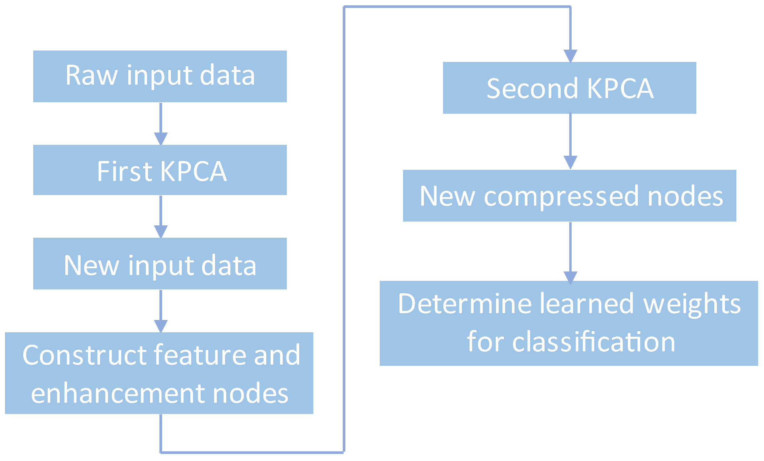
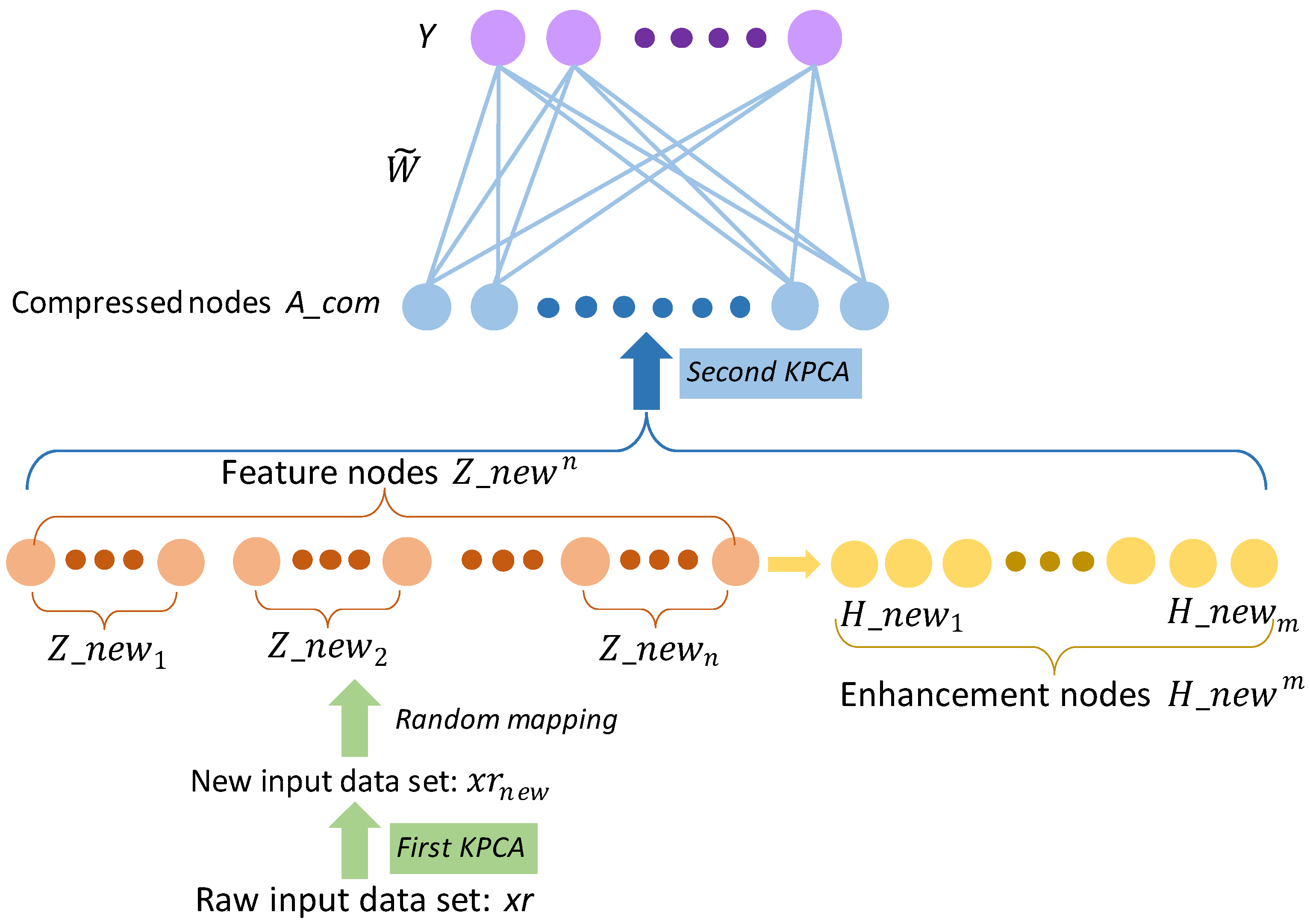
The brief diagram of the proposed BLM_DFE is presented in Figure 2. The raw input data are initially processed with the first KPCA to obtain new input data. Then, these produced new input data containing more compact information can be used to construct feature and enhancement nodes. Thus, all these produced feature/enhancement nodes are further processed with the second KPCA to generate new compressed nodes for calculating the learned weights. These learned weights are applied for classification to evaluate the proposed model. Furthermore, the whole architecture of this model is shown in Figure 3. In detail, the original input training data samples ($xr$) are processed with the first KPCA (green box) to generate new, low-dimensional features (${xr}_{new}$) as the new input for the broad learning model (green arrow displayed in Figure 3). The raw test data samples ($xt$) are also mapped with the first KPCA, as explained in Section 2.3. In this way, we can obtain the new feature nodes (orange circles) and new enhancement nodes (yellow circles) as follows:

$${Z\_new}^n=\left[{Z\_new}_1,{Z\_new}_2,\dots ,{Z\_new}_n\right]$$

(26)

$${H\_new}^m=\left[{H\_new}_1,{H\_new}_2,\dots ,{H\_new}_m\right]$$

(27)

All new feature nodes and enhancement nodes can be used to construct a new matrix as follows:

$$A\_new=\left[{Z\_new}^n\left|{H\_new}^m\right.\right]$$

(28)

Here, we continue to apply KPCA (light-blue box) to process and compress $A\_new$, due to a large number of feature/enhancement nodes within the redundant information. Then, the generated $A\_com$ (the compressed nodes in light-blue circles) are used to calculate the recognition results as follows:

$$Y=A\_com\stackrel{\sim }{W}$$

(29)

The new trainable learned weight matrix ($\stackrel{\sim }{W}$) can be computed in the same way as mentioned in Section 2.1:

$$\stackrel{\sim }{W}={\left({A\_com}^{T}A\_com+\lambda I\right)}^{-1}{A\_com}^{T}Y$$

(30)

where $A\_com$ denotes the compressed nodes, as expressed in Figure 3; Y indicates the label matrix; I signifies the identity matrix; and $\lambda$ represents the regularization parameter. For the test procedures, test samples ${xt}_{new}$ mapped with the first KPCA are processed and generated corresponding to the feature/enhancement nodes, which are further mapped and compressed with the second KPCA and applied to determine the predicted output matrix ($Y_{predict}$) with the learned weight matrix ($\stackrel{\sim }{W}$). Thus, the final predicted class labels can be obtained using $Y_{predict}$.

To sum up, the specific steps of the proposed BLM_DFE can be described as follows:

• Compute the new training data based on KPCA with Equations (9)–(21), and select one kernel among Equations (22)–(24).
• Calculate feature/enhancement nodes (${Z\_new}^n$, ${H\_new}^m$) with Equations (1) and (3) in the broad learning structure.
• Apply the second KPCA to generate $A\_new2$ according to Equations (9)–(21).
• Compute the learned weight matrix ($\stackrel{\sim }{W}$) with Equation (30) for the proposed model.
• Map the raw test data samples based on the first KPCA; map the generated corresponding test feature/enhancement nodes based on the second KPCA with Equation (25).
• Obtain the classification results under the learned weight matrix ($\stackrel{\sim }{W}$) for the test data.

4. Experiments and Analysis

4.1. Experimental Settings

Here, we conducted diverse experiments on various benchmark databases with the proposed BLM_DFE and compared some popular classifiers, including the standard BLS. Specifically, several classification methods, including collaborative representation-based classification (CRC) [44], sparse representation-based classification (SRC) [45], probabilistic collaborative representation-based classifier (ProCRC) [46], least square regression (LSR) [47], k-nearest neighbors (K-NNs) [48], BLS, low-rank ridge regression (LRRR) [49], sparse low-rank regression (SLRR) [49], discriminative LSR (DLSR) [50], FEDLDA [51], and FEMDA [52], and the proposed model were carefully analyzed and assessed. The parameters of these compared classifiers were tuned to achieve competitive results on each database. For the standard BLS, we set 1600 feature nodes and 5000 enhancement nodes for these evaluated databases. For the proposed method, we selected three types of kernels (mentioned in Section 2.3) to implement and perform classification, respectively. These models are denoted by BLM_DFE(RBF), BLM_DFE(sigmoid), and BLM_DFE(linear), which are also abbreviated as BLM_DFE(R), BLM_DFE(S), and BLM_DFE(L).

We randomly selected different sample numbers from each class as the training set (Tr.) from each database, while the rest was regarded as the test set in this study. For the training/test sets, we simulated the processing steps mentioned in Figure 2 as follows: The data samples of the original training set were initially processed with the first KPCA (green box expressed in Figure 3) to generate new training input data. Then, these new training input data were utilized to produce training feature/enhancement nodes based on Equations (1) and (3). Afterwards, the generated training feature/enhancement nodes were processed with the second KPCA to produce compressed training nodes to compute the learned weights. In addition, the first and second KPCAs were also deployed according to Equations (9)–(21). For the data samples in the test set, we also followed the above-mentioned steps to map the original test input data and test feature/enhancement nodes using the first and second KPCAs to produce test compressed nodes. In this way, we calculated the learned weights (from the training phase) with the compressed test nodes to predict the test results. All mentioned classification approaches were repeated 10 times to acquire the final average classification results. Besides this, experiments on the proposed model were implemented on MATLAB 2022a using a PC with a 3.60 GHz CPU and 32 GB RAM.

In this study, we conducted experiments on various types of benchmark databases, including plant, object, face, clothing, and healthcare fields. These databases were applied to evaluate the effectiveness of the proposed model comprehensively. The details of these evaluated databases are expressed as follows: The GT database has 750 facial images from 50 persons (shown in Figure 4a) that were further resized to 40 × 30 grayscale samples for assessment [53]. Each candidate contains 15 samples with various facial expressions. The Flavia database [54] contains 1907 images of 32 leaf species, which were further processed into 40 × 40 grayscale samples for analysis. Each class of leaf contains various lengths, widths, and shapes (shown in Figure 4b). The COIL20 database [55] preserves 1440 grayscale images of 20 classes, which were further resized to 32 × 32 for evaluation (illustrated in Figure 4c). Each class of COIL20 contains 72 images of an object with various orientations. The COIL100 database [56] has 7200 images of 100 objects. Each object contains 72 samples obtained by rotating the object by 5 degrees in each pose interval, and the images were further resized to 32 × 32 grayscale samples for analysis (shown in Figure 4d). The Fashion-MNIST database [57] contains fashion products of 10 classes, such as trousers, dresses, etc. Here, we used a subset of the original database consisting of 2000 images (200 samples per class) [58], which were further processed to 28 × 28 for evaluation (displayed in Figure 4e). In addition, a disease detection database for identifying fatty liver disease (i.e., the FLD database) was also evaluated in this study. This database contains 220 fatty liver disease samples and 220 healthy samples. Each sample contains one facial image (768 × 576) of a candidate and was further processed to obtain facial key blocks before generating the corresponding color feature for analysis. More details about this database can be explored in Ref. [59]. In addition, the information on the above-mentioned databases is explained in

Table 1. The information of the 6 databases used.

Database Name	Num. of Samples	Num. of Classes	Dimensions	Data Type
GT	750	50	40 × 30	Image
Flavia	1907	32	40 × 40	Image
COIL20	1440	20	32 × 32	Image
COIL100	7200	100	32 × 32	Image
Fashion-MNIST	2000	10	28 × 28	Image
FLD	440	2	768	Extracted feature

.

4.2. Experimental Results

The corresponding results of various classification methods are displayed in

Table 2. The results in ARR (%) of various methods on the GT database (best results in bold).

Tr	SRC	CRC	ProCRC	K-NNs	LSR	BLS	FEDLDA
5	65.06	56.86	57.38	65.92	60.84	61.44	60.82
6	69.89	59.49	60.07	69.02	64.42	64.87	64.29
7	72.15	62.10	62.75	70.92	66.03	66.43	65.73
8	74.31	62.43	63.17	73.17	66.54	68.23	68.46
Tr	FEMDA	LRRR	SLRR	DLSR	BLM_DFE(R)	BLM_DFE(S)	BLM_DFE(L)
5	68.42	61.94	61.02	72.34	77.28	74.08	73.72
6	72.93	65.31	64.73	76.33	79.44	77.18	77.00
7	74.38	67.59	67.50	79.05	82.15	80.35	78.52
8	75.43	69.09	68.16	81.49	83.74	81.71	80.91

in terms of the GT database. It can be noted that the proposed BLM_DFE(R) achieved the best accuracy (ARR) compared with other common classifiers by randomly selecting different sample numbers for each class as the training set.

The related experimental results conducted on the Flavia, COIL20, COIL100, Fashion-MNIST, and FLD databases are shown in

Table 3. The results in ARR (%) of various methods on the Flavia database (best results in bold).

Tr	SRC	CRC	ProCRC	K-NNs	LSR	BLS	FEDLDA
4	61.14	55.68	56.05	63.37	55.59	53.88	57.28
5	65.14	57.77	58.29	65.89	57.64	55.67	59.56
6	66.62	58.76	59.24	68.13	58.72	57.12	61.73
7	68.43	59.81	60.13	70.39	59.49	58.32	62.95
Tr	FEMDA	LRRR	SLRR	DLSR	BLM_DFE(R)	BLM_DFE(S)	BLM_DFE(L)
4	65.73	54.99	54.76	64.69	66.81	64.05	62.57
5	68.60	57.92	57.05	67.25	69.14	65.63	67.02
6	71.06	58.42	57.98	68.89	71.07	68.75	68.00
7	73.31	59.86	59.07	71.30	72.26	70.87	70.52

,

Table 4. The results in ARR (%) of various methods on the COIL20 database (best results in bold).

Tr	SRC	CRC	ProCRC	K-NNs	LSR	BLS	FEDLDA
4	80.45	75.96	76.14	80.60	76.76	73.32	79.70
5	83.74	79.87	80.03	84.12	80.17	78.48	81.28
6	85.57	80.58	80.86	85.39	80.61	81.52	84.33
7	87.74	83.22	83.57	87.00	83.45	83.69	85.48
Tr	FEMDA	LRRR	SLRR	DLSR	BLM_DFE(R)	BLM_DFE(S)	BLM_DFE(L)
4	81.85	78.16	77.04	83.04	85.35	84.13	84.97
5	85.59	79.90	79.39	86.29	88.40	87.83	88.16
6	86.61	82.89	81.26	87.72	90.73	90.23	90.69
7	89.15	84.41	82.80	89.42	91.92	92.05	91.69

,

Table 5. The results in ARR (%) of various methods on the COIL100 database (best results in bold).

Tr	SRC	CRC	ProCRC	K-NNs	LSR	BLS	FEDLDA
7	76.63	62.48	63.82	76.12	65.13	73.53	76.85
8	79.23	63.94	65.50	78.39	66.39	76.84	78.56
9	80.68	65.18	66.87	80.31	67.52	79.19	80.44
10	82.13	65.93	67.81	81.30	68.17	81.71	81.40
Tr	FEMDA	LRRR	SLRR	DLSR	BLM_DFE(R)	BLM_DFE(S)	BLM_DFE(L)
7	78.77	65.63	65.23	81.92	83.59	80.19	80.34
8	81.00	66.93	66.19	83.97	85.44	84.63	83.51
9	82.74	67.85	67.62	85.72	86.82	86.24	85.00
10	84.18	68.42	68.31	86.38	87.88	88.32	85.95

,

Table 6. The results in ARR (%) of various methods on the Fashion-MNIST database (best results in bold).

Tr	SRC	CRC	ProCRC	K-NNs	LSR	BLS	FEDLDA
10	70.80	69.05	69.02	65.63	68.34	70.63	61.84
15	73.09	71.58	71.50	66.62	70.65	72.37	63.08
20	75.61	73.47	73.36	69.20	72.15	74.11	64.30
25	77.01	74.52	74.46	69.83	73.54	74.61	65.39
Tr	FEMDA	LRRR	SLRR	DLSR	BLM_DFE(R)	BLM_DFE(S)	BLM_DFE(L)
10	70.48	67.67	67.15	67.26	72.45	71.24	70.76
15	73.27	69.59	69.72	70.79	73.93	74.64	72.30
20	74.76	70.42	70.32	72.08	75.74	75.18	73.64
25	75.95	71.42	71.08	73.19	76.52	76.13	73.89

and

Table 7. The results in ARR (%) of various methods on the FLD database (best results in bold).

Tr	SRC	CRC	ProCRC	K-NNs	LSR	BLS	FEDLDA
20	77.80	77.43	77.40	75.15	71.25	75.28	62.25
30	79.53	79.50	79.45	76.37	72.79	76.63	65.68
40	80.19	80.42	80.44	78.36	73.56	77.94	67.89
50	81.65	81.71	81.76	79.15	75.26	78.76	69.56
Tr	FEMDA	LRRR	SLRR	DLSR	BLM_DFE(R)	BLM_DFE(S)	BLM_DFE(L)
20	76.34	75.13	74.98	73.65	78.15	76.12	74.95
30	78.26	76.94	76.08	74.66	80.61	77.26	76.42
40	79.53	78.47	78.31	75.36	81.39	78.06	77.39
50	80.76	79.32	79.23	76.56	81.97	78.85	78.82

, respectively. The proposed model obtained excellent performance compared with other methods, especially by applying BLM_DFE(R). Besides this, BLM_DFE(S) usually also achieves competitive results in this study. Compared with the standard BLS, the results of our model, e.g., BLM_DFE(R), are often significantly improved here. Therefore, the results in Table 2, Table 3, Table 4, Table 5, Table 6 and Table 7 validate the effectiveness of the proposed model in classification tasks. Overall, it can be observed that applying the RBF kernel in this BLM_DFE model often shows more superiority over other kernels in the experimental results displayed in Table 2, Table 3, Table 4, Table 5, Table 6 and Table 7.

We also performed a brief ablation study to show the usefulness of the dual feature extraction/dimensionality reduction approach with KPCA in BLM_DFE. We implemented and applied KPCA to extract low-dimensional features as the new input for the standard broad learning framework without further processing the feature/enhancement nodes with the second KPCA. This designed model is denoted by KBLM with different kernels, i.e., KBLM(RBF), KBLM(sigmoid), and KBLM(linear). These methods are abbreviated as KBLM(R), KBLM(S), and KBLM(L).

Another alternative method is to only apply the second KPCA to process and compress the feature/enhancement nodes while still keeping the original input samples for the broad learning framework. This developed model is expressed as BLMK with various kernels, i.e., BLMK(RBF), BLMK(sigmoid), and BLMK(linear). More simply, these methods are concisely denoted by BLMK(R), BLMK(S), and BLMK(L), respectively.

To demonstrate the superiority and rationality of the proposed model, we compared BLM_DFE with KBLM, BLMK, and basic BLS on the GT and Flavia databases. The corresponding experimental results are presented in

Table 8. The results in ARR (%) of the ablation analysis on the GT database (best results in bold).

Tr	BLS	KBLM(R)	BLMK(R)	BLM_DFE(R)	KBLM(S)
5	61.44	76.06	70.94	77.28	73.28
6	64.87	79.16	74.87	79.44	76.20
7	66.43	81.90	76.92	82.15	79.35
8	68.23	83.66	78.80	83.74	81.66
Tr	BLMK(S)	BLM_DFE(S)	KBLM(L)	BLMK(L)	BLM_DFE(L)
5	65.46	74.08	72.99	58.44	73.72
6	68.53	77.18	75.84	61.93	77.00
7	71.75	80.35	78.35	63.28	78.52
8	73.06	81.71	81.63	66.17	80.91

and

Table 9. The results in ARR (%) of the ablation analysis on the Flavia database (best results in bold).

Tr	BLS	KBLM(R)	BLMK(R)	BLM_DFE(R)	KBLM(S)
4	53.88	65.86	61.35	66.81	63.25
5	55.67	67.53	65.62	69.14	65.59
6	57.12	68.64	67.39	71.07	69.13
7	58.32	69.83	68.08	72.26	71.02
Tr	BLMK(S)	BLM_DFE(S)	KBLM(L)	BLMK(L)	BLM_DFE(L)
4	59.08	64.05	63.73	53.07	62.57
5	61.38	65.63	66.10	55.38	67.02
6	63.42	68.75	67.33	57.55	68.00
7	63.79	70.87	70.49	57.84	70.52

. It can be easily observed that the proposed model usually obtains outstanding recognition results in these tables. For instance, BLM_DFE(R) achieved an accuracy of 77.28% with five training samples on the GT database and obtained 66.81% in terms of accuracy with four training samples on the Flavia database. Thus, these results also confirm the discriminatory power of $A\_com$ generated based on a dual feature extraction strategy with the KPCA technique.

Here, we utilized the random forest classifier to evaluate the generated $A\_com$ and computed its corresponding feature importance scores for further assessment [60]. In particular, we applied the BLM_DFE(R) model on the GT database with five training samples to produce the corresponding $A\_com$ features. Then, we used the random forest method to analyze the generated $A\_com$ to retrieve the corresponding importance scores, as shown in Figure 5a. The horizontal axis represents the number of input features ($A\_com$), while the vertical axis represents the importance score of each input feature. Moreover, we also followed this strategy to evaluate the Flavia database with four training samples and computed its feature importance scores, as displayed in Figure 5b. From Figure 5, it can be observed that each input feature is effective for prediction, with the first few dozen features being very important for prediction. These results are consistent with the KPCA technique, which can process raw input data and calculate the principal components as generated features. In addition, we discuss the settings of the number of principal components for KPCA to ensure that the generated $A\_com$ is optimal and effective in Section 4.3.

We chose the classification results (five samples per class as the training set in the GT database displayed in Table 2) for further evaluation. The accuracy of the proposed model was utilized to compare the accuracy using the standard BLS by performing the t-test [61]. We also followed this strategy for evaluating the accuracy results on other databases (4, 4, 7, 10, 20 samples per class as the training sets in the Flavia, COIL20, COIL100, Fashion-MNIST, FLD databases) for assessment. The corresponding results of the p-value are expressed in

Table 10. The p-value of our BLM_DFE versus standard BLS on various databases.

Database	GT	Flavia	COIL20	COIL100	Fashion-MNIST	FLD
p-Value	$1.91\times {10}^{-13}$	$2.29\times {10}^{-13}$	$9.79\times {10}^{-13}$	$1.24\times {10}^{-12}$	$1.55\times {10}^{-3}$	$1.43\times {10}^{-3}$

. It can be observed that these p-value results represent the statistically significant difference in BLM_DFE compared with the original BLS in terms of accuracy on different databases.

4.3. Parameter Analysis

In BLM_DFE, several parameters should be carefully tuned to show the desired classification results. For instance, parameter $\lambda$ in Equation (30) is used to compute the learned weights. The parameters of the kernel, such as $\gamma$, in Equation (22) are utilized in KPCA. The number of principal components, i.e., $PCN$, is set in KPCA. Since we implement and insert KPCA twice in the broad learning structure, if we select the RBF kernel, there are five parameters, i.e., $\lambda$, (${\gamma }_{KPCA1}$, ${PCN}_{KPCA1}$) of the first KPCA, and (${\gamma }_{KPCA2}$, ${PCN}_{KPCA2}$) of the second KPCA, that need to be adjusted. To the best of our knowledge, investigating and finding the optimal parameters represent an open issue in various applications [62,63,64]. Here, we employed the same number of feature/enhancement nodes and other settings used in the standard BLS mentioned in Section 4.1, while only parameters $\lambda$, $\gamma$, and $PCN$ were evaluated and selected to explore the optimal combinations step by step.

In our work, we fixed other parameters while evaluating parameter $\lambda$, as shown in Figure 6a. It can be observed that our model was insensitive to parameter $\lambda$ in the range of [${10}^{-12}$–${10}^{-4}$] and obtained suitable performance. Afterwards, we fixed parameter $\lambda$ and investigated parameters ${\gamma }_{KPCA1}$, ${PCN}_{KPCA1}$, as shown in Figure 6b. We can find that our model achieved satisfactory results with ${\gamma }_{KPCA1}$ and ${PCN}_{KPCA1}$ located at ${10}^{-2}$ and in the range of [60–100], respectively. In this way, we continued to evaluate ${\gamma }_{KPCA2}$, ${PCN}_{KPCA2}$ when others were fixed, as shown in Figure 6c. It can be noted that parameters ${\gamma }_{KPCA2}$, ${PCN}_{KPCA2}$ are located in the ranges of [${10}^{-6}$–${10}^{-3}$] and [180–240], respectively, guaranteeing reasonable performance. In this way, we can roughly explore the optimal parameters of the proposed model. For other kernels and other databases, we also investigated them using a similar strategy to acquire the corresponding optimal parameters for performing classification.

4.4. Computing Time

Here, we chose the GT and Flavia databases to analyze and evaluate the whole computation time of the proposed BLM_DFE(R) and other popular classification approaches. The parameter settings were kept the same as mentioned in Section 4.1. The corresponding results are shown in

Table 11. The computing time of various classification methods on the GT database with 5 training samples.

Method	SRC	CRC	ProCRC	K-NNs	LSR	BLS
Computing time (s)	2.29	0.52	0.18	0.09	0.01	4.65
Method	FEDLDA	FEMDA	LRRR	SLRR	DLSR	BLM_DFE(R)
Computing time (s)	1.08	24.48	1.03	1.65	0.21	2.57

and

Table 12. The computing time of various classification methods on the Flavia database with 4 training samples.

Method	SRC	CRC	ProCRC	K-NNs	LSR	BLS
Computing time (s)	4.33	1.16	0.47	0.11	0.01	4.89
Method	FEDLDA	FEMDA	LRRR	SLRR	DLSR	BLM_DFE(R)
Computing time (s)	0.87	16.13	1.06	1.74	0.15	2.87

. Although the computation time can be longer compared with the comparison methods, such as LSR, it is still acceptable when considering its competitive recognition results mentioned in Table 2 and Table 3.

From Section 3, it can be found that the main computational overheads of the BLM_DFE model are computing the learned weight matrix ($\stackrel{\sim }{W}$) (Equation (30)) and two-KPCA processing, while the computational costs of other calculations are negligible and insignificant. Considering that we have n input samples as the training set, L indicates the number of feature/enhancement nodes of the original BLS; c represents the number of classes of the input samples; and p denotes the number of compressed nodes of BLM_DFE. Thus, the complexity of two-KPCA processing is $O\left(2n^3\right)$. The complexity of computing Equation (30) is $O\left(p^3+n{p}^2+n{p}^2+pnc\right)$, where $O\left(p^3\right)$ represents the cost of matrix inversion operation and $O\left(n{p}^2+n{p}^2+pnc\right)$ denotes the cost of several matrix multiplication operations. Thus, the overall computational complexity of the proposed BLM_DFE can be represented as $O\left(2n^3+p^3+n{p}^2+n{p}^2+pnc\right)$. The main computational cost of the original BLS is to calculate the learned weight matrix (W) (Equation (5)), which has computational complexity of $O\left(L^3+n{L}^2+n{L}^2+Lnc\right)$. Compared with the basic BLS, the computational complexity of the proposed model mainly depends on the two additional KPCA processes, resulting in a higher computational overhead when the number of input samples (n) is large. However, due to the use of KPCA to compress the number of feature/enhancement nodes, p is usually much smaller than L, resulting in our model having advantages in computational overhead on small- and medium-sized datasets. The comparison of computational time (BLS versus BLM_DFE) in Table 11 and Table 12 also reflects this point.

5. Discussion

We have designed and developed a novel method that imposes KPCA on the broad learning framework to improve recognition performance. The novel outcomes of this BLM_DFE can be presented as follows: Our model can process the original input data and generate feature/enhancement nodes to obtain more effective features as well as simplify the architecture of broad learning. Furthermore, by applying various kernels of KPCA, this dual feature extraction approach shows its effectiveness in the experimental results shown in Table 2, Table 3, Table 4, Table 5, Table 6 and Table 7. For instance, it can be seen that the proposed model with an RBF kernel obtains the accuracy of 83.74%; with the sigmoid kernel, it achieves 81.71% accuracy; with the linear kernel, it produces 80.91% accuracy; all under 8 training samples on the GT database. Although the results of applying different kernels are different, they also prove the superiority of the proposed model. For example, K-NNs, as one comparison method, only achieved 73.17% accuracy under the same experimental settings. The reason that the proposed model can improve the classification performance compared with the original BLS and other methods can be expressed as follows: Applying KPCA can obtain more effective feature representation compared with the original high-dimensional data. Besides this, compressing a large number of raw feature/enhancement nodes and transforming them into another feature space can reduce redundant nodes and preserve useful information. Given these points, researchers can consider implementing their own models to obtain better recognition results based on the proposed dual feature extraction strategy in terms of high-dimensional input data or features already extracted using learning models in real-world applications.

From the above-mentioned experimental results (Table 2, Table 3, Table 4, Table 5, Table 6 and Table 7), it can be observed that the performance of BLM_DFE(L) is usually worse than that of BLM_DFE(R) and BLM_DFE(S). The reason is that BLM_DFE(L) uses a linear kernel, rather than the RBF or sigmoid kernel applied in BLM_DFE(R) and BLM_DFE(S), which can perform nonlinear dimension reduction and often achieve more competitive performance. Thus, these related experimental results also confirm the effectiveness of the KPCA applied in the proposed model.

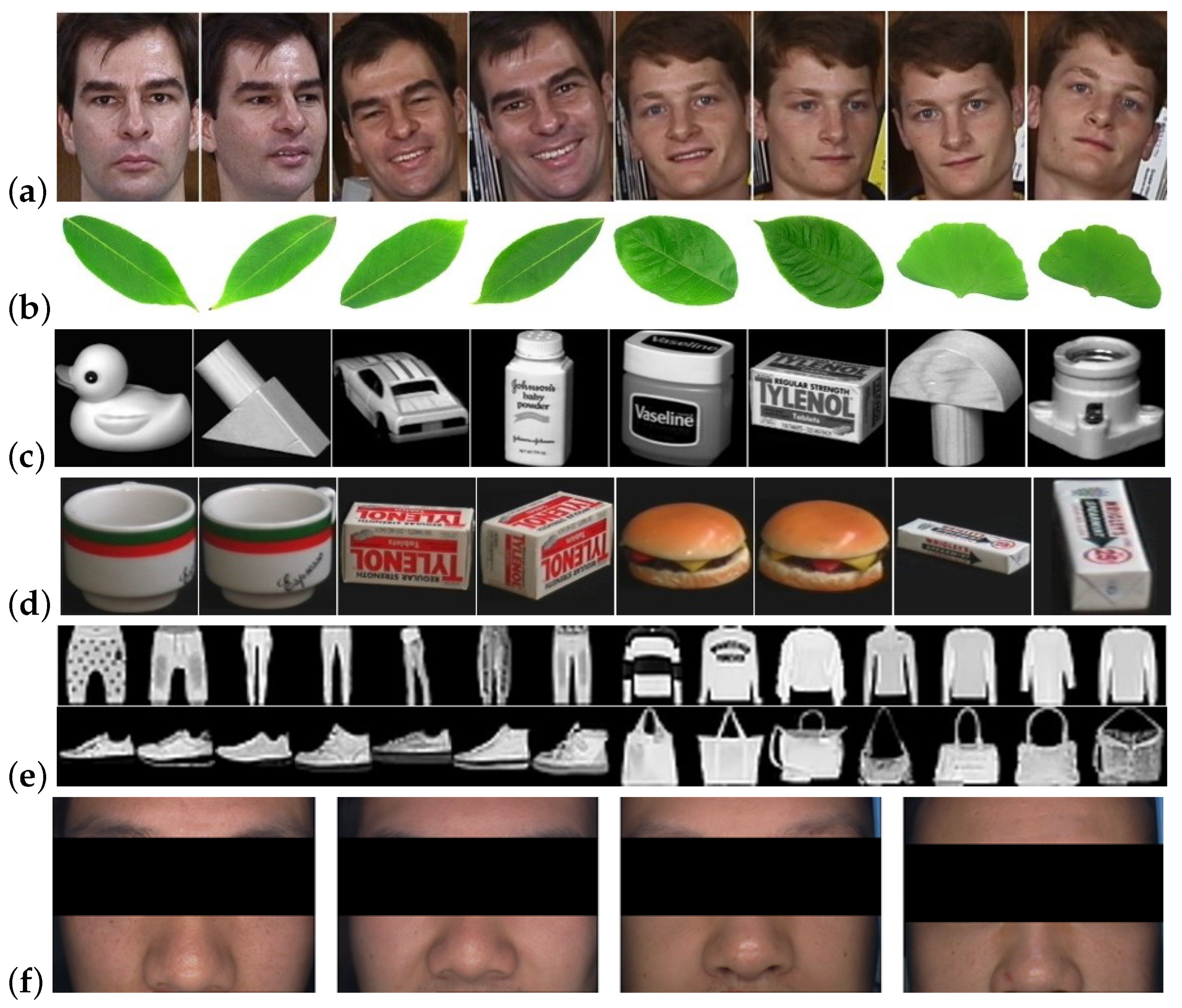
We evaluated the proposed BLM_DFE on six different databases. Our model achieved significant improvements in the data types of face, plant, and object compared with the original BLS (refer to Table 2, Table 3, Table 4 and Table 5). Since this model achieved good results on face, plant, and object data types, we could consider handling practical applications similar to these mentioned data types, such as flowers, in future investigations.

In the ablation study, we compared the proposed model with several reduced models implemented by ourselves, such as KBLM and BLMK. From the experimental results in Table 8 and Table 9, we can find that the dual feature extraction strategy showed excellent performance. The performance of the linear kernel used in the proposed model often showed inferiority with respect to the other kernels, such as RBF. This evidence illustrates that nonlinear KPCA can obtain effective features and perform dimensionality reduction on more complicated structures of input data. In addition, although the results of BLMK are inferior to those of KBML and BML_DFE, this model is still competitive and achieved good results on the described databases. For instance, BLMK with an RBF kernel attained the accuracy of 67.39% compared with LRRR, which obtained 58.42% accuracy when employing six training samples on the Flavia database. Considering this, BLMK could simplify the structure of the BLS with fewer nodes for classification, making BLM_DFE also inherit this advantage in recognition applications. The results of this ablation study teach us that a large number of nodes may have redundant information. Hence, it is a meaningful way to compress these nodes in classification tasks. Moreover, to further verify the effectiveness of the generated $A\_com$, we plan to apply the acquired $A\_com$ features with other popular classifiers, such as SVM, for evaluation in future studies. Thus, we can assess whether $A\_com$ can further improve the classification performance when employed together with other common models, which can explore and enhance the novelty of the proposed model.

In this study, we attempt to insert the KPCA technique into a broad learning structure to address some issues mentioned above (e.g., redundant information among feature/enhancement nodes) in the standard BLS and further enhance its classification performance. The KPCA technique is embedded in the broad learning architecture, rather than simply being combined with it. Besides this, some recent studies [17,25] also adopted similar strategies to modify the basic BLS and improved their proposed models’ performance, as expressed in the Introduction section. Therefore, although the proposed model is relatively simple in terms of technical soundness, considering the obvious improvement in experimental results on various benchmark databases and related studies by other researchers, we believe this work is still meaningful in terms of novelty.

The advantages of the proposed model are very obvious and clear, as mentioned in the previous sections. However, there is still room for improvement in the proposed model. For instance, KPCA is a quite popular and widely used feature extraction method that has been validated in various studies and applications. Thus, we selected KPCA to extract the low-dimensional useful features as the new input in the broad learning framework. Valid high-level information in the extracted raw input data may be ignored. Hence, integrating other feature extraction methods, such as stacked autoencoder [65], to generate multiple features as the new input may further enhance classification performance. Given this point, we aim at exploring and investigating a multi-feature extraction broad learning model in our future studies. There are some disadvantages to our BLM_DFE. For instance, when using KPCA to process data, we need to address an $N\times N$ matrix (with N indicating the number of input samples), and the computational complexity is $O\left(N^3\right)$, which is also expressed in Section 4.4. Therefore, if the number of input samples is very large, the computational cost of KPCA is also high. Considering this point, the proposed model is more suitable for dealing with classification tasks with small- or medium-sized databases. The original BLS has a good ability to process and evolve new input data in classification applications. Another shortcoming of this BLM_DFE model is that the embedding and processing of KPCA change the raw input data or original feature/enhancement nodes, affecting its ability to dynamically deal with new input data. However, it is still acceptable when considering the superior performance of the proposed model on various databases compared with other popular classifiers, including the standard BLS. In addition, we aim to further explore ameliorating this model to have a better capability to dynamically process data in the future.

Here, we introduced a dual feature extraction strategy by applying KPCA embedded in the broad learning structure to handle high-dimensional input data and feature/enhancement nodes, which adds several transformation operations. One of the main issues is that these operations can make the fine tuning and understanding of this model more complex. However, the KPCA technique can compress feature/enhancement nodes to obtain concise and valuable features, which are used to compute the learned weight matrix using ridge regression as in the standard BLS. Therefore, we only need to embed multiple KPCA operations in building this model while not significantly increasing the complexity of this model structure. In addition, we validated our implemented model on various real-world databases. The corresponding experimental results also verify the rationality and usability of our model in practical classification applications.

6. Conclusions

In this paper, we illustrated a novel broad learning model with a dual feature extraction strategy for classification applications. Compared with the raw input data and original feature/enhancement nodes used in the basic broad learning framework, the proposed model can exploit the effective low-dimensional features with the raw input data and compress the used nodes to simultaneously simplify the structure of the broad learning architecture. In this way, we can accomplish ideal classification results by imposing this dual feature strategy on the broad learning model. Related experimental results on various benchmark databases confirm the effectiveness of the proposed model compared with other popular classification approaches, including the basic BLS. Moreover, further investigation and amelioration of the proposed model to enhance the feature extraction ability or flexible data processing ability are desired in future studies.

References

1. Alpaydin, E. Introduction to Machine Learning; MIT Press: Cambridge, MA, USA, 2020. [Google Scholar]
2. Zhou, Z.H. Machine Learning; Springer Nature: Singapore, 2021. [Google Scholar]
3. LeCun, Y.; Bengio, Y.; Hinton, G. Deep learning. Nature 2015, 521, 436–444. [Google Scholar] [CrossRef] [PubMed]
4. He, K.; Zhang, X.; Ren, S.; Sun, J. Deep residual learning for image recognition. In Proceedings of the IEEE Conference on Computer Vision and Pattern Recognition, Las Vegas, NV, USA, 27–30 June 2016; pp. 770–778. [Google Scholar]
5. Zhang, Q.; Zhou, J.; Xu, Y.; Zhang, B. Collaborative representation induced broad learning model for classification. Appl. Intell. 2023, 1–15. [Google Scholar] [CrossRef]
6. Chen, C.P.; Liu, Z. Broad learning system: An effective and efficient incremental learning system without the need for deep architecture. IEEE Trans. Neural Netw. Learn. Syst. 2017, 29, 10–24. [Google Scholar] [CrossRef]
7. Pao, Y.H.; Park, G.H.; Sobajic, D.J. Learning and generalization characteristics of the random vector functional-link net. Neurocomputing 1994, 6, 163–180. [Google Scholar] [CrossRef]
8. Gong, X.; Zhang, T.; Chen, C.P.; Liu, Z. Research review for broad learning system: Algorithms, theory, and applications. IEEE Trans. Cybern. 2021, 52, 8922–8950. [Google Scholar] [CrossRef] [PubMed]
9. Yang, Y.; Huang, Q.; Li, P. Online prediction and correction control of static voltage stability index based on Broad Learning System. Expert Syst. Appl. 2022, 199, 117184. [Google Scholar] [CrossRef]
10. Fan, W.; Si, Y.; Yang, W.; Sun, M. Class-specific weighted broad learning system for imbalanced heartbeat classification. Inf. Sci. 2022, 610, 525–548. [Google Scholar] [CrossRef]
11. Gan, J.; Xie, X.; Zhai, Y.; He, G.; Mai, C.; Luo, H. Facial beauty prediction fusing transfer learning and broad learning system. Soft Comput. 2023, 27, 13391–13404. [Google Scholar] [CrossRef]
12. Xu, L.; Chen, C.P.; Qing, F.; Meng, X.; Zhao, Y.; Qi, T.; Miao, T. Graph-Represented Broad Learning System for Landslide Susceptibility Mapping in Alpine-Canyon Region. Remote Sens. 2022, 14, 2773. [Google Scholar] [CrossRef]
13. Cao, Y.; Jia, M.; Zhao, X.; Yan, X.; Liu, Z. Semi-supervised machinery health assessment framework via temporal broad learning system embedding manifold regularization with unlabeled data. Expert Syst. Appl. 2023, 222, 119824. [Google Scholar] [CrossRef]
14. Feng, S.; Chen, C.P. Fuzzy broad learning system: A novel neuro-fuzzy model for regression and classification. IEEE Trans. Cybern. 2018, 50, 414–424. [Google Scholar] [CrossRef]
15. Jin, J.; Qin, Z.; Yu, D.; Li, Y.; Liang, J.; Chen, C.P. Regularized discriminative broad learning system for image classification. Knowl. Based Syst. 2022, 251, 109306. [Google Scholar] [CrossRef]
16. Du, J.; Vong, C.M.; Chen, C.P. Novel efficient RNN and LSTM-like architectures: Recurrent and gated broad learning systems and their applications for text classification. IEEE Trans. Cybern. 2020, 51, 1586–1597. [Google Scholar] [CrossRef] [PubMed]
17. Yang, K.; Liu, Y.; Yu, Z.; Chen, C.P. Extracting and composing robust features with broad learning system. IEEE Trans. Knowl. Data Eng. 2021, 35, 3885–3896. [Google Scholar] [CrossRef]
18. Li, T.; Fang, B.; Qian, J.; Wu, X. Cnn-based broad learning system. In Proceedings of the 2019 IEEE 4th International Conference on Signal and Image Processing (ICSIP), Wuxi, China, 19–21 July 2019; pp. 132–136. [Google Scholar]
19. Chen, L.; Li, M.; Lai, X.; Hirota, K.; Pedrycz, W. CNN-based broad learning with efficient incremental reconstruction model for facial emotion recognition. IFAC Pap. 2020, 53, 10236–10241. [Google Scholar] [CrossRef]
20. Sheng, B.; Li, P.; Zhang, Y.; Mao, L.; Chen, C.P. GreenSea: Visual soccer analysis using broad learning system. IEEE Trans. Cybern. 2020, 51, 1463–1477. [Google Scholar] [CrossRef]
21. Chu, Y.; Lin, H.; Yang, L.; Sun, S.; Diao, Y.; Min, C.; Fan, X.; Shen, C. Hyperspectral image classification with discriminative manifold broad learning system. Neurocomputing 2021, 442, 236–248. [Google Scholar] [CrossRef]
22. Wu, G.; Duan, J. BLCov: A novel collaborative–competitive broad learning system for COVID-19 detection from radiology images. Eng. Appl. Artif. Intell. 2022, 115, 105323. [Google Scholar] [CrossRef] [PubMed]
23. Zhou, Y.; She, Q.; Ma, Y.; Kong, W.; Zhang, Y. Transfer of semi-supervised broad learning system in electroencephalography signal classification. Neural Comput. Appl. 2021, 33, 10597–10613. [Google Scholar] [CrossRef]
24. Zhan, C.; Jiang, W.; Lin, F.; Zhang, S.; Li, B. A decomposition-ensemble broad learning system for AQI forecasting. Neural Comput. Appl. 2022, 34, 18461–18472. [Google Scholar] [CrossRef]
25. Zhao, H.; Zheng, J.; Xu, J.; Deng, W. Fault diagnosis method based on principal component analysis and broad learning system. IEEE Access 2019, 7, 99263–99272. [Google Scholar] [CrossRef]
26. Wen, J.; Deng, S.; Fei, L.; Zhang, Z.; Zhang, B.; Zhang, Z.; Xu, Y. Discriminative regression with adaptive graph diffusion. IEEE Trans. Neural Netw. Learn. Syst. 2022. [Google Scholar] [CrossRef] [PubMed]
27. Salah, M.B.; Yengui, A.; Neji, M. Feature extraction and selection in archaeological images for automatic annotation. Int. J. Image Graph. 2022, 22, 2250006. [Google Scholar] [CrossRef]
28. Jolliffe, I.T.; Cadima, J. Principal component analysis: A review and recent developments. Philos. Trans. R. Soc. A Math. Phys. Eng. Sci. 2016, 374, 20150202. [Google Scholar] [CrossRef]
29. Xie, X.; Lam, K.M. Gabor-based kernel PCA with doubly nonlinear mapping for face recognition with a single face image. IEEE Trans. Image Process. 2006, 15, 2481–2492. [Google Scholar]
30. Bishop, C.M.; Nasrabadi, N.M. Pattern Recognition and Machine Learning; Springer: New York, NY, USA, 2006. [Google Scholar]
31. Hargrove, L.J.; Li, G.; Englehart, K.B.; Hudgins, B.S. Principal components analysis preprocessing for improved classification accuracies in pattern-recognition-based myoelectric control. IEEE Trans. Biomed. Eng. 2008, 56, 1407–1414. [Google Scholar] [CrossRef] [PubMed]
32. Howley, T.; Madden, M.G.; O’Connell, M.L.; Ryder, A.G. The effect of principal component analysis on machine learning accuracy with high dimensional spectral data. In Proceedings of the International Conference on Innovative Techniques and Applications of Artificial Intelligence, Cambridge, UK, 12–14 December 2005; pp. 209–222. [Google Scholar]
33. Wang, Q. Kernel principal component analysis and its applications in face recognition and active shape models. arXiv 2012, arXiv:1207.3538. [Google Scholar]
34. Schölkopf, B.; Burges, C.J.; Smola, A.J. Advances in Kernel Methods: Support Vector Learning; MIT Press: Cambridge, MA, USA, 1999. [Google Scholar]
35. Wu, J.; Wang, J.; Liu, L. Feature extraction via KPCA for classification of gait patterns. Hum. Mov. Sci. 2007, 26, 393–411. [Google Scholar] [CrossRef]
36. Fauvel, M.; Chanussot, J.; Benediktsson, J.A. Kernel principal component analysis for the classification of hyperspectral remote sensing data over urban areas. EURASIP J. Adv. Signal Process. 2009, 2009, 783194. [Google Scholar] [CrossRef]
37. Shao, R.; Hu, W.; Wang, Y.; Qi, X. The fault feature extraction and classification of gear using principal component analysis and kernel principal component analysis based on the wavelet packet transform. Measurement 2014, 54, 118–132. [Google Scholar] [CrossRef]
38. Gong, M.; Liu, J.; Li, H.; Cai, Q.; Su, L. A multiobjective sparse feature learning model for deep neural networks. IEEE Trans. Neural Netw. Learn. Syst. 2015, 26, 3263–3277. [Google Scholar] [CrossRef]
39. Hoerl, A.E.; Kennard, R.W. Ridge regression: Biased estimation for nonorthogonal problems. Technometrics 1970, 12, 55–67. [Google Scholar] [CrossRef]
40. Schölkopf, B.; Smola, A.; Müller, K.R. Nonlinear component analysis as a kernel eigenvalue problem. Neural Comput. 1998, 10, 1299–1319. [Google Scholar] [CrossRef]
41. Kim, K.I.; Franz, M.O.; Scholkopf, B. Iterative kernel principal component analysis for image modeling. IEEE Trans. Pattern Anal. Mach. Intell. 2005, 27, 1351–1366. [Google Scholar] [PubMed]
42. Weinberger, K.Q.; Sha, F.; Saul, L.K. Learning a kernel matrix for nonlinear dimensionality reduction. In Proceedings of the Twenty-First International Conference on Machine Learning, Banff, AB, Canada, 4–8 July 2004; p. 106. [Google Scholar]
43. Schölkopf, B.; Smola, A.; Müller, K.R. Kernel principal component analysis. In Proceedings of the International Conference on Artificial Neural Networks, Lausanne, Switzerland, 8–10 October 1997; pp. 583–588. [Google Scholar]
44. Zhang, L.; Yang, M.; Feng, X. Sparse representation or collaborative representation: Which helps face recognition? In Proceedings of the 2011 International Conference on Computer Vision, Barcelona, Spain, 6–13 November 2011; pp. 471–478. [Google Scholar]
45. Wright, J.; Yang, A.Y.; Ganesh, A.; Sastry, S.S.; Ma, Y. Robust face recognition via sparse representation. IEEE Trans. Pattern Anal. Mach. Intell. 2008, 31, 210–227. [Google Scholar] [CrossRef] [PubMed]
46. Cai, S.; Zhang, L.; Zuo, W.; Feng, X. A probabilistic collaborative representation based approach for pattern classification. In Proceedings of the IEEE Conference on Computer Vision and Pattern Recognition, Las Vegas, NV, USA, 27–30 June 2016; pp. 2950–2959. [Google Scholar]
47. Zhang, Q.; Zhang, B. Low Rank Based Discriminative Least Squares Regression with Sparse Autoencoder Processing for Image Classification. In Proceedings of the 2021 7th International Conference on Computer and Communications (ICCC), Chengdu, China, 10–13 December 2021; pp. 836–840. [Google Scholar]
48. Fukunaga, K.; Narendra, P.M. A branch and bound algorithm for computing k-nearest neighbors. IEEE Trans. Comput. 1975, 100, 750–753. [Google Scholar] [CrossRef]
49. Cai, X.; Ding, C.; Nie, F.; Huang, H. On the equivalent of low-rank linear regressions and linear discriminant analysis based regressions. In Proceedings of the 19th ACM SIGKDD International Conference on Knowledge Discovery and Data Mining, Chicago, IL, USA, 11–14 August 2013; pp. 1124–1132. [Google Scholar]
50. Xiang, S.; Nie, F.; Meng, G.; Pan, C.; Zhang, C. Discriminative least squares regression for multiclass classification and feature selection. IEEE Trans. Neural Netw. Learn. Syst. 2012, 23, 1738–1754. [Google Scholar] [CrossRef]
51. Yang, J.; Sun, Q.S.; Yuan, Y.H. Feature extraction using fractional-order embedding direct linear discriminant analysis. Neural Process. Lett. 2018, 48, 1583–1595. [Google Scholar] [CrossRef]
52. Houdouin, P.; Wang, A.; Jonckheere, M.; Pascal, F. Robust classification with flexible discriminant analysis in heterogeneous data. In Proceedings of the ICASSP 2022-2022 IEEE International Conference on Acoustics, Speech and Signal Processing (ICASSP), Virtual, 7–13 May 2022; pp. 5717–5721. [Google Scholar]
53. Chen, L.; Man, H.; Nefian, A.V. Face recognition based on multi-class mapping of Fisher scores. Pattern Recognit. 2005, 38, 799–811. [Google Scholar] [CrossRef]
54. Wu, S.G.; Bao, F.S.; Xu, E.Y.; Wang, Y.X.; Chang, Y.F.; Xiang, Q.L. A leaf recognition algorithm for plant classification using probabilistic neural network. In Proceedings of the 2007 IEEE International Symposium on Signal Processing and Information Technology, Giza, Egypt, 15–18 December 2007; pp. 11–16. [Google Scholar]
55. Nene, S.A.; Nayar, S.K.; Murase, H. Columbia object image library (coil-20). 1996. Available online: https://www1.cs.columbia.edu/CAVE/publications/pdfs/Nene_TR96.pdf (accessed on 2 August 2023).
56. Nene, S.A.; Nayar, S.K.; Murase, H. Columbia object image library (coil 100). 1996. Available online: https://www1.cs.columbia.edu/CAVE/publications/pdfs/Nene_TR96_2.pdf (accessed on 2 August 2023).
57. Xiao, H.; Rasul, K.; Vollgraf, R. Fashion-mnist: A novel image dataset for benchmarking machine learning algorithms. arXiv 2017, arXiv:1708.07747. [Google Scholar]
58. Zhou, J.; Zeng, S.; Zhang, B. Sparsity-induced graph convolutional network for semisupervised learning. IEEE Trans. Artif. Intell. 2021, 2, 549–563. [Google Scholar] [CrossRef]
59. Zhang, Q.; Wen, J.; Zhou, J.; Zhang, B. Missing-view completion for fatty liver disease detection. Comput. Biol. Med. 2022, 150, 106097. [Google Scholar] [CrossRef]
60. Kuhn, M.; Johnson, K. Applied Predictive Modeling; Springer: New York, NY, USA, 2013. [Google Scholar]
61. Ruxton, G.D. The unequal variance t-test is an underused alternative to Student’s t-test and the Mann–Whitney U test. Behav. Ecol. 2006, 17, 688–690. [Google Scholar] [CrossRef]
62. Wen, J.; Xu, Y.; Li, Z.; Ma, Z.; Xu, Y. Inter-class sparsity based discriminative least square regression. Neural Netw. 2018, 102, 36–47. [Google Scholar] [CrossRef] [PubMed]
63. Fang, X.; Teng, S.; Lai, Z.; He, Z.; Xie, S.; Wong, W.K. Robust latent subspace learning for image classification. IEEE Trans. Neural Netw. Learn. Syst. 2017, 29, 2502–2515. [Google Scholar] [CrossRef]
64. Wen, J.; Zhang, Z.; Fei, L.; Zhang, B.; Xu, Y.; Zhang, Z.; Li, J. A survey on incomplete multiview clustering. IEEE Trans. Syst. Man Cybern. Syst. 2022, 53, 1136–1149. [Google Scholar] [CrossRef]
65. Wang, Y.; Liu, M.; Bao, Z.; Zhang, S. Stacked sparse autoencoder with PCA and SVM for data-based line trip fault diagnosis in power systems. Neural Comput. Appl. 2019, 31, 6719–6731. [Google Scholar] [CrossRef]
Figure 1. The standard architecture of broad learning. The feature/enhancement nodes are constructed to compute the learned weight (W).
Mathematics 11 04087 g001
Figure 2. The basic diagram of the proposed BLM_DFE for classification.
Mathematics 11 04087 g002
Figure 3. The architecture of the proposed BLM_DFE. It utilizes a dual feature extraction strategy to process raw input data and map feature/enhancement nodes with KPCA. Here, W indicates the trainable learned weights computed from the compressed nodes, while Y denotes the corresponding labels.
Mathematics 11 04087 g003
Figure 4. Typical samples of various databases, including (a) GT, (b) Flavia, (c) COIL20, (d) COIL100, (e) Fashion-MNIST, (f) FLD.
Mathematics 11 04087 g004
Figure 5. The bar chart of applying random forest classifier to compute feature importance scores with A _ c o m generated from the BLM_DFE(R) model on the (a) GT database and (b) Flavia database.
Mathematics 11 04087 g005aMathematics 11 04087 g005b
Figure 6. The classification accuracy (%) results with various combinations of parameters to evaluate (a) parameter λ , (b) parameters γ K P C A 1 , P C N K P C A 1 , (c) parameters γ K P C A 2 , P C N K P C A 2 on the GT database with 5 training samples per class.
Mathematics 11 04087 g006