Abstract
Reducing carbon emissions and improving revenue in the face of global warming and economic challenges is a growing concern for airlines. This paper addresses the inefficiencies and high costs associated with current aero-engine on-wing washing strategies. To tackle this issue, we propose a reinforcement learning framework consisting of a Similar Sequence Method and a Taylor DQN model. The Similar Sequence Method, comprising a sample library, DTW algorithm, and boundary adjustment, predicts washed aero-engine data for the Taylor DQN model. Leveraging the proposed Taylor neural networks, our model outputs Q-values to make informed washing decisions using data from the Similar Sequence Method. Through simulations, we demonstrate the effectiveness of our approach.
Keywords:
aircraft engine cleaning schedule; reinforcement learning; Taylor DQN model; similar sequence method MSC:
90B35; 68B05; 74P10
1. Introduction
On-wing washing is one of the maintenance tasks for aero-engines, which involves using high-end washing equipment to remove deposits from the surfaces of aero-engine air passages. These deposits originate from air pollutants that are ingested by the aero-engine [1]. Accumulated deposits can reduce the airflow into the engine, leading to incomplete combustion of fuel and increased fuel consumption and carbon emissions, ultimately raising exhaust temperatures [2].
Aero-engine on-wing washing can restore fuel efficiency and reduce carbon emissions by eliminating the build-up of dirt. In 2023, the world faced a serious problem of fuel scarcity and extreme weather conditions caused by greenhouse gas emissions. Therefore, washing has been widely recognized and applied in many countries around the world. On-wing washing is listed as a mandatory item in the maintenance schedule.
Due to the high cost of washing, airlines need to consider “when to wash” the aero-engine (i.e., washing strategy) according to economic and environmental benefits. Therefore, the washing strategy for aero-engines has significant research value. The cost of renting high-end washing equipment required for aero-engine washing is very high, so frequent washing is not feasible. Ref. [3] studies on washing gas turbines have found the cost of washing to be prohibitively high and, therefore, not recommended. However, aero-engines must be washed to ensure flight safety [4,5,6]. Therefore, airlines need a reasonable washing strategy to carefully balance the benefits and carbon emissions issues.
Early research on washing strategies focused on gas turbine washing in power plants. Fuel flow and economic costs were the main points of concern for such studies. A Fabbri et al. [7] used gas turbines as their research objects and designed a washing frequency based on fuel flow, production power, fuel costs, and maintenance costs. R. Klassen [8] developed washing frequencies for aircraft bases based on economic parameters and local atmospheric environments to reduce maintenance costs. F. S. Spüntrup et al. [9] proposed short-term washing strategies for gas turbines to reduce carbon emissions and increase operational profits. Dan et al. [10] developed washing frequencies with the goal of reducing fuel consumption.
In the aviation industry, the Exhaust Gas Temperature Margin (EGTM) is to develop aero-engine washing strategies for maintenance bases [11]. In some maintenance bases, EGTM is used as the sole indicator of the effectiveness of engine washing. Exhaust Gas Temperature refers to the temperature at the low-pressure turbine outlet of the aircraft engine. Engine manufacturers provide a red line value for Exhaust Gas Temperature. When Exhaust Gas Temperature rises to the red line value, the engine will be in a highly dangerous state, and flight safety cannot be guaranteed [12]. EGTM refers to the distance between the Exhaust Gas Temperature and the red line value, where a greater distance indicates greater safety. Another commonly mentioned physical quantity in this paper is “Flight cycle”, which is a time unit used in the field of aircraft maintenance. A cycle refers to a period of time from one takeoff to the next takeoff, including takeoff, cruise, descent, and landing. Figure 1 illustrates that the value of EGTM is relatively high when the engine is freshly manufactured. EGTM will gradually decay to zero without any maintenance measures taken [13,14]. Figure 2 shows that EGTM will quickly recover after being cleaned [15,16]. The images reflect that EGTM is highly sensitive to cleaning.
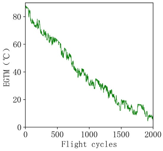
Figure 1.
EGTM of never-washed engine.
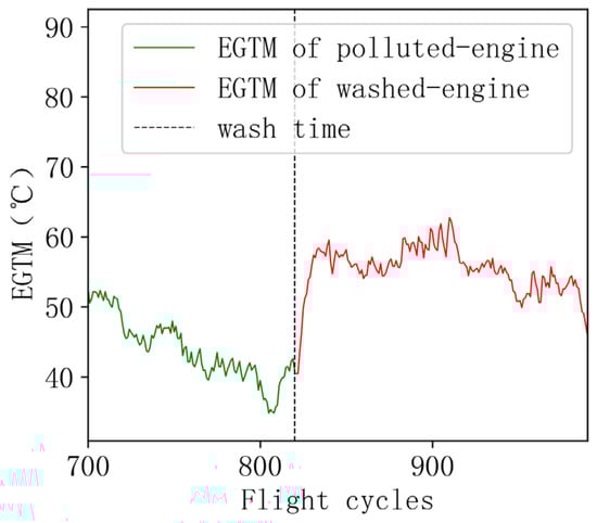
Figure 2.
EGTM of washed engine.
Similarly, research in academia on aircraft engine washing strategies focuses on the recovery level of EGTM. Zhu et al. [17] proposed a washing frequency based on Weibull methods through EGTM data fitting. Fu et al. [18] established an evaluation model for the engine washing effect based on EGTM data and evaluated the washing effect based on this model. Yan et al. [19] established a transfer process neural network to predict washed aero-engine EGTM data.
However, both the gas turbine washing strategies and aircraft engine washing strategies lack adaptability to changing operating conditions. These washing strategies are developed based on fixed, known operating scenarios and belong to “static optimization”. When the operating conditions of the aero-engines change frequently, these optimization plans need to be modified accordingly. The above methods cannot choose the appropriate washing time based on real-time observations of the current status of the aero-engine to generate washing strategies that are more targeted, efficient, and cost-effective.
Reinforcement learning (RL) can achieve adaptive washing strategies. Reinforcement learning is a machine learning method used to solve the problem of how agents learn policies to maximize profits through interactions with the environment. Romain Gautron et al. [20] describe the application prospects of RL methods in crop management. Seongmun Oh et al. [21] used RL methods to improve the balance between energy storage system supply and demand, thereby adjusting the electricity usage time reasonably and reducing production costs. Yanting Zhou et al. [22] proposed an improved deep RL method to achieve energy scheduling and promote carbon neutrality. Leonardo Kanashiro Felizardoa et al. [23] use RL algorithms to observe information about the market, such as financial reports, news, asset price time series, and financial indicators, to make sound financial trading decisions.
However, RL methods demonstrate low learning efficiency [24]. RL algorithms rely on trial-and-error explorations of the environment to discover optimal policies. This process can be time-consuming and require a large number of interactions with the environment. The reward signal used in RL can be sparse or delayed, which means that the agent may not receive any feedback on the quality of its actions until much later. This makes it difficult for the agent to estimate which actions led to rewards and optimize its policy accordingly [25].
Therefore, a substantial amount of pre- and post-washing aero-engine data is required to achieve optimization of the washing schedule. Furthermore, due to limited aero-engine data availability, a generative model that can simulate pre- and post-washing aero-engine data is necessary. Currently, there is a scarcity of evaluation methods for the post-washing status of aero-engines, thus resulting in a lack of existing methods that can serve as generative models.
To address the aforementioned issues, a proposed optimization method for aero-engine washing strategy is presented in this paper, as illustrated in Figure 3.
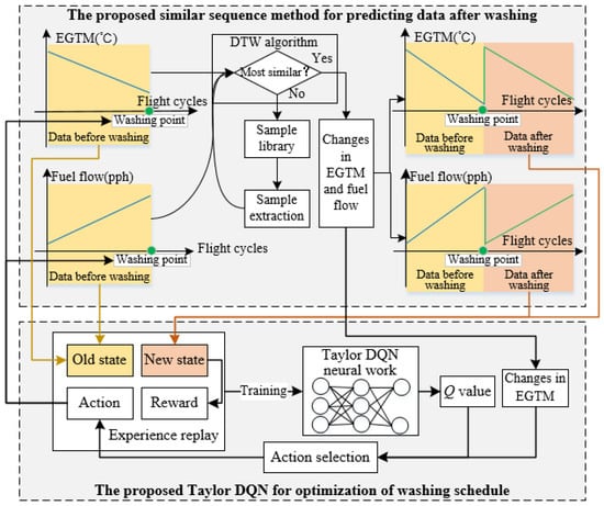
Figure 3.
The proposed optimization method for aero-engine washing strategy.
Figure 3 depicts that the proposed optimization method for aero-engine washing strategy consists of two parts, namely, the Similar Sequence Method and the Taylor Deep Q-Network (DQN) for optimization.
The Similar Sequence Method serves as the generative model for reinforcement learning. As reinforcement learning suffers from inefficient data utilization, the data acquired from airlines cannot satisfy the data requirements of reinforcement learning. Thus, we propose the Similar Sequence Method to generate sufficient data.
The Similar Sequence Method computes the changes in the Exhaust Gas Temperature Margin (EGTM) and fuel flow after washing, which are used to provide new states for the Taylor DQN. The sample library stored in the Similar Sequence Method contains data changes before and after washing. The DTW algorithm is employed to compare the similarity of EGTM data and fuel flow data before washing with the sample library data and select the most similar data corresponding to the changes in EGTM and fuel flow for computing the data after washing.
The proposed Taylor DQN framework consists of three main components: experience replay, the Taylor neural network, and action selection.
Experience Replay: Experience replay is a memory buffer that stores the history of interactions between the agent (the washing strategy optimizer) and the environment (the aero-engine). The stored data include the old state (pre-washing data), new state (post-washing data), action taken, and corresponding reward. By randomly sampling and replaying these experiences during training, the agent can utilize past experiences for more effective learning.
Taylor Neural Network: The Taylor neural network is a key component of the Taylor DQN model. It utilizes Taylor decomposition, a mathematical technique used for approximating functions, to decompose input information from experience replay into key feature information. By doing so, it obtains valuable insights and patterns necessary for optimizing the washing schedule. The Taylor neural network processes the pre-washing and post-washing data and outputs Q-values that represent the expected future rewards for different actions. These Q-values serve as the basis for action selection in the optimization process.
To summarize, the problem faced by cleaning optimization is that existing methods lack adaptability to constantly changing operating conditions and rely on static optimization plans, which cannot provide targeted, efficient, and cost-effective cleaning strategies based on real-time observation of the current state of aviation engines. In addition, the amount of relevant data is limited and cannot support the RL method. To address these issues, this paper makes two main contributions:
Firstly, the Similar Sequence Method is proposed for predicting data after washing. This method combines the sample library with the DTW algorithm to obtain the changes in EGTM and fuel flow by seeking similar data, thereby computing the data of the washed aero-engine.
Secondly, the proposed Taylor neural network is introduced for providing the Q-value for action selection. The Taylor neural network is a model based on Taylor decomposition that decomposes input information from experience replay to obtain key feature information in the form of the Q-value output.
2. The Proposed Similar Sequence Method
This section introduces the Similar Sequence Method for predicting data after washing, as shown in Figure 4.
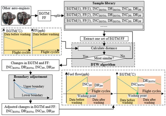
Figure 4.
The proposed Similar Sequence Method for predicting data after washing.
Figure 4 shows that the proposed Similar Sequence Method includes three parts: sample library, DTW algorithm, and boundary adjustment.
In our proposed Similar Sequence Method, the main objective is to predict data after washing based on the available information. Our method comprises three main components: the sample library, DTW algorithm, and boundary adjustment. These components work together to predict the changes in Exhaust Gas Temperature Margin (EGTM) and fuel flow (FF) after washing. The sample library plays a crucial role by storing EGTM data, FF data, and related parameters, such as INC|EGTM, DR|EGTM, INC|FF, and DR|FF. These parameters capture the changes in EGTM and FF after washing.
The DTW algorithm is then employed to search for the most similar data from the sample library to the “data before washing” sequence. This allows us to estimate the corresponding changes in EGTM and FF after the engine has undergone washing.
To make the estimation closer to reality, we introduced the boundary adjustment technique. By collecting local extreme points of washed EGTM and FF data from other aero-engines of the same model and grouping them based on time, we can determine upper bounds, lower bounds, and mean curves for EGTM and FF recovery. These boundaries provide us with realistic ranges for the changes in EGTM and FF.
By adjusting the predicted values based on these boundaries, we ensure that the predicted data after washing align with real-world conditions. If the predicted values exceed the upper bound or fall below the lower bound, they are corrected to the mean value. These adjustments improve the accuracy of the predictions and mitigate the data scarcity problem to some extent.
2.1. Sample Library
The sample library stores EGTM data, FF data, INC|EGTM, DR|EGTM, INC|FF, and DR|FF. The fuel flow data are defined as “ff”. Let the aero-engine fuel flow dataset be marked as ff: {fft}, where “t” refers to the flight cycle. Mark the washing record as Twashing: {ti, i = 1, 2, ……, n–1}. The elements in Twashing correspond to the flight cycles when the aero-engine was washed. “i” refers to the number of washes. Twashing can split the ff data into n groups, labeled as:
INC|FF and DR|FF are obtained by fitting linear equations to the data in Equation (1). After the “i-th” wash, INCi|FF and DRi|FF are obtained by fitting the data ff (i + 1), using:
where Length(ff(i + 1)) refers to the length of ff(i + 1).
Similarly, the EGTM data are defined as “e”. Let the aero-engine fuel flow dataset be marked as e: {et}. Twashing can split the e data into n groups, labeled as:
INC|EGTM and DR|EGTM are obtained by fitting linear equations to the data in Equation (3). For the “i-th” wash, INCi|EGTM and DRi|EGTM are obtained by fitting the data e (i + 1), using:
Since there is no corresponding INC and DR for the “n-th” group of e and ff data, the sample library stores n–1 groups of data, which can be obtained from Equation (5).
2.2. Dynamic Time Warping (DTW) Algorithm
The Similar Sequence Method utilizes the DTW algorithm to calculate the distance between the “data before washing” and all data in the expert library, thereby enabling the prediction of changes in Exhaust Gas Temperature Margin (EGTM) and fuel flow (FF). DTW is a dynamic programming algorithm commonly used to measure the similarity between two time series data. It considers the non-linear variations and different lengths of time series.
In the context of the Similar Sequence Method, the DTW algorithm allows for the comparison and selection of the most similar data from the expert library. This is crucial for accurately predicting the changes in EGTM and FF after washing. By considering the non-linear variations and different lengths of time series through the DTW algorithm, the Similar Sequence Method improves the prediction accuracy.
The proposed method, which utilizes the DTW algorithm within the similar sequence framework, is applied to calculate the distance between the “data before washing” and all data in the expert library. Once the minimum distance is found, the corresponding EGTM and FF changes from the expert library are outputted.
The DTW algorithm is a dynamic programming algorithm used for measuring the similarity between two time series data. It can be used to compare the distance between two time series and find the shortest path. The DTW algorithm can handle time series of different lengths, and also adapts well to cases with non-linear variations.
The key formula of the DTW algorithm is the dynamic programming equation, which is used to calculate the distance between two time series. The dynamic programming equation of the DTW algorithm is as follows: [26]
where D (k, l) indicates the minimum distance between the first “k” elements of the “data before washing” sequence and the first “l“ elements of the sample library’s ff or e. “d (k, l)” represents the Euclidean distance between the “k-th” element of the “data before washing” sequence and the “l-th” element of the sample library’s ff or e.
The set of distances between “data after washing” and all ff (i), e(i) is then solved: .
The output corresponds to the minimum “Di” value, which is linked to the “changes in EGTM and FF”.
The recovery of EGTM and FF after the washing of the aero-engine has a range, which is obtained through boundary adjustment aiming to ensure that changes in EGTM and FF correspond to reality. This paper defines the upper bound, lower bound, and mean curve for this range, as shown in Figure 5.
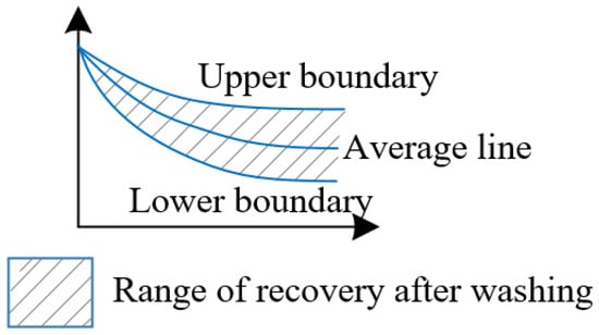
Figure 5.
Schematic diagram of boundary.
2.3. Boundary Adjustment
This paper collected the local extreme points of washed EGTM and FF data from other aero-engines of the same model. These extreme points were grouped based on time using the K-means algorithm. The maximum value, minimum value, and average value of each group were calculated and fitted as the upper bound, lower bound, and mean line to adjust changes in EGTM and FF. The revised flowchart is shown in Figure 6.
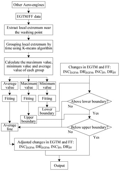
Figure 6.
Data correction process.
This paper used clustering algorithms to divide all extreme points into seven areas according to time T, expressed as T1, T2, ……, T7. For the aero-engine’s EGTM data, let eT represent all EGTM data extreme points in the T area. The EGTM mean value dataset is defined by Equation (8):
By using t as the independent variable, the EGTM data mean curve can be defined as:
where a0, b0, d0, and g0 are model parameters fitted by the dataset .
The element set emax within the upper bound of EGTM is defined by Equation (10):
The upper bound function of EGTM is defined by Equation (11):
where a1, b1, d1, and g1 are model parameters obtained by fitting the dataset emax.
The element set emin within the lower bound of EGTM for the aero-engine is defined by Equation (12):
The lower bound function of EGTM is defined by Equation (13):
where a2, b2, d2, and g2 are model parameters obtained by fitting the dataset emin.
Let ffT represent all FF data extreme points in the T time area, then the FF mean value dataset ffave is defined by Equation (14):
The FF mean curve is defined by Equation (15):
where a4, b4, d4, and g4 are model parameters obtained by fitting the dataset ffmax.
The element set ffmax within the upper bound of FF is defined by Equation (16):
The upper bound function of FF is defined by Equation (17):
where a4, b4, d4, and g4 are model parameters obtained by fitting the dataset ffmax.
The element set ffmin within the lower bound of FF is defined by Equation (18):
The lower bound function of FF is defined by Equation (19):
where a5, b5, d5, and g5 are model parameters obtained by fitting the dataset ffmin.
In the t-th flight cycle, INC|EGTM and INC|FF are calculated, and the following adjustments are made using boundary conditions:
- (1)
- When INC|EGTM > fup(t)|EGTM or INC|EGTM < fdown(t)|EGTM, the value of INC|EGTM is corrected to fave(t)|EGTM.
- (2)
- Similarly, when INC|FF > fup(t)|FF or INC|FF < fdown(t)|FF, the value of INC|FF is corrected to fave(t)|FF.
Based on the above, the updates for EGTM and FF data are as follows:
- (1)
- If the engine obtains INCi|EGTM and DRi|EGTM after the i-th washing at time t0, then e: {et} after t0 is updated as:
- (2)
- Similarly, for ff: {fft}, the updated FF data after t0 are:
In summary, after obtaining these upper bounds, lower bounds, and mean curves for both EGTM and FF, adjustments are made to the predicted values of INC|EGTM and INC|FF based on the boundary conditions. If the predicted value exceeds the upper bound or falls below the lower bound, it is corrected to the mean value. The adjustments are made using Equations (11), (13), (17), and (19). Based on these adjustments, the EGTM and FF data are updated using Equations (20) and (21), respectively.
The boundary adjustment process calculates the upper bounds, lower bounds, and mean curves for EGTM and FF recovery after washing the aero-engine. These boundaries are necessary to ensure the changes in EGTM and FF align with real-world conditions. By using these boundaries to adjust the predicted values, the accuracy of the predictions is improved, leading to more reliable results.
The processes of the Similar Sequence Method for post-washing data prediction are as follows:
Step 1: Sample library creation
The sample library is established to provide materials for finding similar data of data after washing. The database contains four parameters: INC|EGTM, DR|EGTM, INC|FF, and DR|FF, which represent the changes and decay rates in EGTM and FF after water washing.
Step 2: Splitting data into groups
The “Twashing” records, representing the flight cycles when the aero-engine was washed, are used to split the FF and EGTM data into n groups. Each group corresponds to a specific wash cycle.
Step 3: Calculation of incremental and decay values
Linear equations are fitted to the FF and EGTM data within each group to obtain parameters, such as INC|EGTM, DR|EGTM, INC|FF, and DR|FF. These parameters represent the changes and decay rates for EGTM and FF after each wash cycle.
Step 4: Dynamic Time Warping (DTW) algorithm
The DTW algorithm is employed to search for similar sequences in the sample library. The DTW algorithm compares the data before washing with all the data in the expert library to find the most similar EGTM and FF sequences. The algorithm considers non-linear variations and different lengths of time series, improving the prediction accuracy.
Step 5: Distance calculation and output
The DTW algorithm calculates the distance between the “data before washing” and all data in the expert library. The minimum distance value obtained corresponds to the most similar sequence, which provides predictions for changes in EGTM and FF.
Step 6: Boundary adjustment
The boundary adjustment process aims to ensure that the predicted changes in EGTM and FF align with real-world conditions. Local extreme points of washed EGTM and FF data from other aero-engines of the same model are collected, grouped based on time using clustering algorithms. Maximum values, minimum values, and average values are calculated for each group and used to define upper bounds, lower bounds, and mean curves. Predicted values of INC|EGTM and INC|FF are adjusted based on boundary conditions, correcting values that exceed the upper bound or fall below the lower bound.
Step 7: Updating EGTM and FF data
After applying boundary adjustments, the EGTM and FF data are updated based on the corrected predicted values. Equations provided in this paper (Equations (20)–(23)) outline the specific updates for EGTM and FF data.
3. The Proposed Taylor DQN Model for Optimization of Washing Schedule
The Taylor DQN comprises five components: action, state, experience replay, Taylor DQN neural network, and Q-value. The relationship among these five components is illustrated in Figure 7.
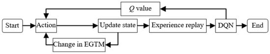
Figure 7.
Learning process of DQN.
As shown in Figure 7, an action is selected based on the Q-value and change in EGTM. The selected action then upgrades the current state, which is subsequently stored in the experience replay. This provides training data for the Taylor DQN neural network.
The experience replay stores four types of data: action, reward, old state, and new state. The two possible actions are “wash” and “no wash,” while the reward represents the earnings of the aero-engine in the new state. Old state refers to the aero-engine state before the action was taken, while new state refers to the state after the action. These states comprise six categories of data: VBW|EGTM, INC|EGTM, DR|EGTM, VBW|FF, INC|FF, and DR|FF. These six categories of data are used as input for training the Taylor DQN neural network.
INC|EGTM and INC|FF denote the step changes in EGTM data and fuel flow data after washing the engine, respectively. These parameters are utilized in engineering to reflect the cleaning efficiency. DR|EGTM and DR|FF refer to the linear decay rates of EGTM data and fuel flow data, respectively, after washing the engine. DR|EGTM and DR|FF are employed in engineering to reflect the long-term effect of washing on the EGTM and fuel flow of aero-engines. VBW|EGTM denotes the value of EGTM before washing, while VBW|FF represents the value of fuel flow before washing. VBW|EGTM and VBW|FF serve as parameters used in engineering to reflect the pre-washing state of aero-engines. These six types of data are the essential basis for cleaning decisions. Therefore, this paper utilizes the Taylor DQN neural network to learn these six types of data, to provide a reference for the make action’s Q-value in advance.
3.1. Taylor DQN Neural Network
We propose the Taylor DQN neural network to extract crucial information from the state and output it in the form of Q-values. The Taylor network estimates the first-order Taylor expansion of the state data. Compared to existing neural network models, the Taylor network has stronger interpretability.
The Taylor DQN neural network extracts key information from the current state and outputs the Q-value for each action, as shown in Figure 8.
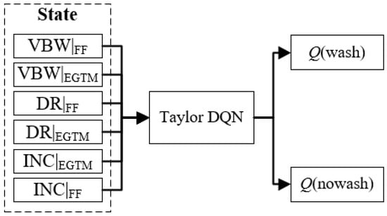
Figure 8.
Input and output of Taylor DQN neural network.
The Taylor DQN neural network performs a first-order Taylor expansion of the input state, discarding the truncation error, while retaining the critical information. The network’s weighted input is defined as wx + b, with its output being f (wx + b). When f (wx + b) is differentiable at wx, f (wx + b) can be expanded at wx:
where f(wx) + f′(wx) ((wx + b) − wx) represents the key information extracted from the state data, and o ((wx + b) − wx) is the useless information that cannot be described by regular rules. Therefore, using f(wx) + f′(wx) ((wx + b) − wx) as key information, Equation (25) can be stated as:
Due to the fast convergence rate of the activation function tanh, this paper chooses the tanh function as f (wx + b), with the activation function tanh determined by Equation (26).
Expanding Equation (26) at wx yields Equation (27):
Equation (27) depicts the Taylor neuron with tanh, as shown in Figure 9.
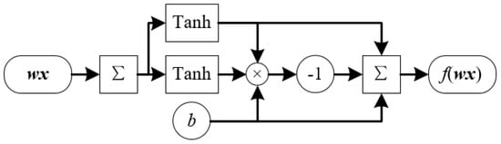
Figure 9.
Taylor neurons with tanh.
The backpropagation of the Taylor neuron with tanh can be solved using the chain rule. The gradient of b in Figure 9 can be calculated by Equation (28).
Similarly, the gradient of w can be calculated by Equation (29).
The Taylor neural network has a three-layer structure, as shown in Figure 10.
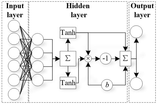
Figure 10.
Taylor neural network model.
The input layer is a fully connected layer that compresses the input information. The hidden layer is a Taylor neuron layer that extracts key information from the compressed data. The output layer outputs the key information in the form of Q-values. Based on the input and output data, the number of nodes in the input layer (nin) and output layer (nout) are six and two, respectively. The number of nodes in the middle layer (nhid) can be obtained using the empirical formula in [27].
Based on the Taylor neural network, the Taylor DQN model is constructed, as shown in Figure 11.
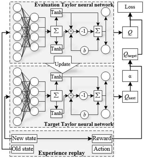
Figure 11.
Taylor DQN model.
Figure 11 shows that two proposed Taylor neural networks are used as the evaluation Taylor neural network and the target network, with the same network structure. The evaluation Taylor neural network takes the old state in the experience replay as input and outputs Q. The target Taylor neural network takes the new state in the experience replay as input and outputs Qnext. Qtarget is calculated using Qnext and Reward.
where α is the learning rate.
The loss function is calculated based on Qtarget and Q.
3.2. Action Selection
The actions in the Taylor DQN model consist of two options: “wash” and “no-wash”. Let A = {‘wash’, ‘no-wash’}.
The model determines whether to wash the aero-engine by evaluating the change in EGTM data after washing. The research conducted by airlines indicates that if the increase in EGTM data is more than 15 °C, the washing was done too late. If the increase in EGTM data is less than 10 °C, the washing was done too early.
Based on the research results, this paper designs the following guidelines for action selection: (1) choose ‘wash’ if the predicted increase in EGTM data after washing exceeds 15 °C; (2) choose ‘no wash’ if the predicted increase in EGTM data after washing is less than 10 °C; (3) if the predicted increase in EGTM data after washing is greater than 10 °C, but less than 15 °C, according to reference [18], we set a 90% probability of deciding whether or not to wash based on the Q-value outputted by the DQN and a 10% chance of randomly selecting an action. The action selection process is shown in Figure 12.
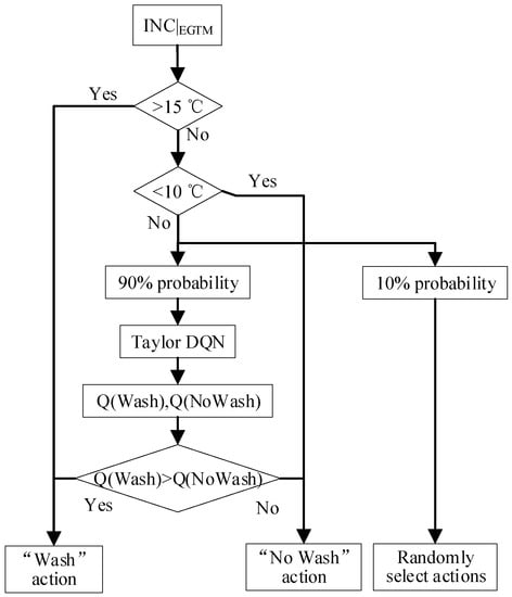
Figure 12.
Action selection.
3.3. Reward
This study centers around the Airbus A320 aircraft as the object of research. The term “Reward” in the text refers to the revenue generated during a specific flight cycle. When the flight cycle is denoted by c and the action as Ac, Rc (Ac) specifies the Reward. When Ac = ‘wash’, Rc (Ac) includes flight revenue, carbon emissions tax, fuel tax, and washing costs:
In Equation (33), income refers to the revenue of a single aero-engine flight. The average duration of a flight cycle for the A320 aircraft is two hours [28]. The revenue of an aircraft is USD 10,549 per hour [29]. Based on on-site research, the washing operation fee is about USD 180,000. The income of a single aero-engine can be deemed as half of the income of an aircraft; thus, the income equals USD 10,549. The tax refers to the carbon emissions tax, which is set at USD 10 (USD/ton):
where EXH represents the amount of carbon emissions, expressed as:
where CEI denotes the carbon emission index, which has a value of 3.153 [10]. According to reference [30], the Average flight time is 2 h, therefore:
In Equation (33), costoil reflects the fuel cost of the engine:
where the fuel cost is USD 0.75 (USD/kg) [31], thus:
When Ac = ‘no wash’, the revenue of the flight cycle includes the flight revenue, carbon emissions tax, and fuel tax, namely:
4. Experiments
This section includes two contents: Boundary Conditions of Aero-Engine State Model, and validation of the optimization effect of reinforcement learning framework based on DQN. Among them, the Boundary Conditions of Aero-Engine State Model modifies the prediction results of the proposed Similar Sequence Method. Due to the reinforcement learning framework using the proposed Similar Sequence Method to calculate action rewards, this paper first completes the fitting of the correction function and then evaluates the optimization effect of the reinforcement learning framework.
The experiment was completed in a Python environment, with the CPU platform being Core2Duo at 2.80 GHz. The data in this paper are collected from real data of a certain engine model. This section arranges a comparison with three cleaning schemes, DQN, Q-learning [18], and Reliability [9], to examine their carbon emissions, company revenue, cleaning frequency, and fuel savings. Finally, the experimental results were analyzed. The EGTM data of the engine come from the outlet temperature of the low-pressure turbine; the FF data of the engine come from the aircraft’s fuel level indicator system. The system installs a set of capacitive probes in the fuel tank to measure the fuel level, and a density gauge sensor is installed in the inner fuel tank of each wing to calculate the fuel quantity.
In this study, the relevant data of the aircraft engine after cleaning required for the model are shown in Table 1.

Table 1.
Relevant data after aero-engine washing.
4.1. Boundary Conditions of Aero-Engine State Model
In order to obtain the formula parameters for the average line and upper and lower boundaries, this study collected data from four aero-engines, spanning from the time of manufacturing to decommissioning. This paper used K-means to divide the data into seven groups, calculating the mean, maximum, and minimum values for each group. Figure 13a shows the fitting results for fave(t)|EGTM, fup(t)|EGTM, and fdown(t)|EGTM. The computed results for fave(t)|FF, fup(t)|FF, and fdown(t)|FF are displayed in Figure 13b. The seven sets of data in Figure 13 are marked with seven different colors.
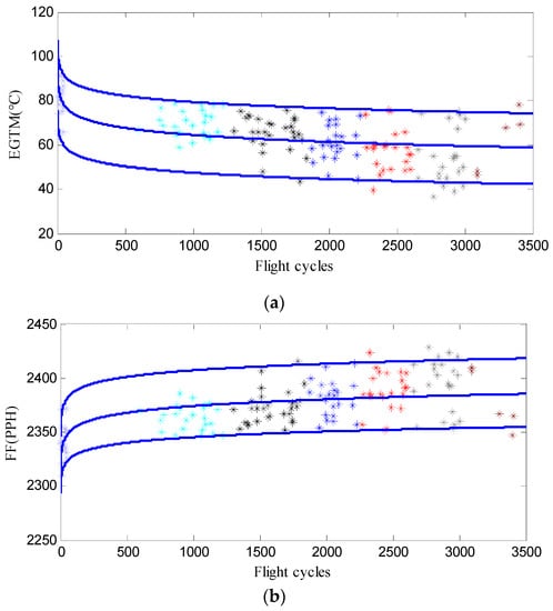
Figure 13.
Fitting results of average line, upper boundary, and lower boundary. (a) Fitting curve of fave(t)|EGTM, fup(t)|EGTM, and fdown(t)|EGTM. (b) Fitting curve of fave(t)|FF, fup(t)|FF, and fdown(t)|FF.
The data presented in Figure 13 can reflect that the restoration of EGTM and fuel flow after aero-engine washing is concentrated in a fixed area. A logarithmic function will be applied to fit the data. The upper boundary formula for EGTM data can be fitted as:
The lower boundary formula for EGTM data can be fitted as:
The performance average descent curve for EGTM data can be fitted as:
Similarly, for FF data, their upper boundary formula can be fitted as:
The lower boundary formula for FF data can be fitted as:
The performance average descent curve for FF data can be fitted as:
4.2. Other Washing Strategy
This paper involves four washing strategies: the real washing strategy provided by the airline company, the Taylor DQN-based washing strategy, the DQN-based washing strategy, and the reliability-based washing strategy. The real washing strategy was obtained from the data provided by the airline company, while the Taylor DQN method was introduced in Section 3. The other two washing strategies are described as follows:
A. Washing strategy based on DQN
A three-layer neural network-based DQN is established as a comparative solution for the Taylor DQN in this paper. Based on the three-layer neural network, the DQN takes six states as input and outputs Q(wash) and Q(no-wash). According to Equation (30), the number of nodes in the middle layer is set to 4. The activation function of the hidden layer is set to ReLU, while the output layer uses the linear function. The optimizer is Adam, and the loss function is the mean squared error. The training process of DQN is the same as that of Taylor DQN.
B. Washing strategy based on Q-learning
Reference [20] combines the Mixed transfer process neural network with Q-learning for optimizing washing strategies. The optimization strategy for Q-learning is as follows:
C. Weibull distribution approaches
Reference [17] established a reliability formula based on EGTM data to guide washing strategies. Let x denote the washing cycle, which refers to the time of several flight cycles. WB denotes the Weibull distribution function, which is determined by Equation (47):
where λ denotes the scale, and k denotes the shape.
The physical meaning of WB is the frequency of occurrence of washing cycles. The washing records of the airline are statistically analyzed into WB probability, as shown in Table 2:
Table 2.
Frequency of WB for the washing period.
By substituting the data of Table 2 into Equation (47), a = 10.41 and b = 1.79 are obtained. Therefore, the washing cycle formula can be derived as follows [17]:
where 1 − WB represents reliability. If the airline company requires a reliability of 1 − WB = 99%, then x = 49.94 ≈ 50. Thus, it is recommended to wash every 50 flight cycles.
4.3. Comparison of Washing Strategies and Methods
Table 3 presents the cleaning benefits of a single aero-engine in 2750 flights under four different cleaning strategies. These benefits include the total number of cleanings, average EGTM, fuel savings, reduced carbon emissions, and increased profits. Fuel savings refer to the difference between the fuel consumption of the current strategy and that of the actual strategy. Reduced carbon emissions refer to the difference between the carbon emissions of the current strategy and those of the actual strategy. Increased profits denote the difference between the total profits of the current strategy and those of the actual strategy.
Table 3.
The washing effect of the three optimization schemes.
Table 3 reveals that Taylor DQN recommends 1 more washing cycle than DQN and 4 more than Q-learning, but 39 cycles less than the Weibull method and 10 more cycles than The Real Strategy. Furthermore, Taylor DQN’s average EGTM is 0.4 °C higher than DQN’s and 6.0 °C higher than Q-learning’s, but 0.2 °C lower than the Weibull method and 4.3 °C higher than The Real Strategy. In addition, Taylor DQN saves 1.97 tons more fuel than DQN, 25.89 tons more fuel than Q-learning, and 1.01 tons less than the Weibull method. Taylor DQN also brings in USD 6307 more profit than DQN, USD 25,490 more profit than Q-learning, and USD 51,960 more profit than the Weibull method.
It can be inferred from Table 3 that Taylor DQN’s strategy is more fuel-efficient, emits fewer carbon emissions, and has lower cleaning costs than DQN’s strategy and Q-learning’s strategy, ultimately leading to greater profitability. Therefore, in this task, the Taylor DQN model outperforms the DQN model and the Q-learning model.
Table 3 reflects that although the benefits brought by traditional DQN are lower than those of Taylor DQN, they are higher than those of Q-learning. The recommended cleaning frequency for traditional DQN is three times more than that learned by Q. The Average EGTM of traditional DQN is 5.6 °C higher than that of Q-learning. Traditional DQN saves 17.47 tons of fuel compared to Q-learning. Traditional DQN reduces carbon emissions by 95.54 tons compared to Q-learning. The benefits brought by traditional DQN are USD 19,183 more than those of Q-learning.
Table 3 indicates that the Weibull method achieved a marginal improvement through frequent cleaning, but at the cost of significant profit losses. Therefore, the Weibull method is not suitable for this task. By using Taylor neural networks to enhance learning ability, Taylor DQN achieves a high degree of EGTM with fewer cleaning cycles. Although the Weibull method maintains the highest degree of EGTM and fuel efficiency throughout the entire process, its cleaning approach results in lower economic benefits compared to the Taylor DQN method.
4.4. Discussion of Results
Our experimental results demonstrate both convergence and divergence when compared to previous research. Converging with prior studies, we found that regular engine cleaning can lead to improvements in EGTM and fuel efficiency and reduced carbon emissions. This aligns with the consensus in the literature that proper maintenance and cleaning contribute to enhanced engine performance.
However, there are also notable divergences between our results and some previous research findings. For instance, in comparison with the reliability-based washing strategy, our Taylor DQN model recommended fewer cleaning cycles, while maintaining a high degree of EGTM and achieving significant fuel savings. This differs from the Weibull method, which suggests more frequent cleaning at the cost of reduced profitability. This discrepancy may be attributed to differing methodologies, datasets, or assumptions used in previous studies.
It is important to note that our study has certain limitations. The data collected for analysis were specific to a particular engine model, and the experiments were conducted under controlled conditions. Therefore, the convergence or divergence of our results with previous research may be influenced by these factors.
Overall, our findings demonstrate both alignment and disparities with previous research. These differences indicate the potential of our proposed Taylor DQN model to outperform traditional methods, such as DQN and Q-learning, in terms of fuel efficiency, carbon emissions reduction, and profitability. Further research and comparative analyses with a broader range of engine models and real-world data would be valuable in establishing the generalizability and robustness of our results.
There are some key factors contributing to the superior performance of the Taylor DQN model:
Complex Input Data Utilization: The model makes use of complex input data involving six different categories: VBW|EGTM, INC|EGTM, DR|EGTM, VBW|FF, INC|FF, and DR|FF. These data points, which reflect various parameters before and after washing the aero-engine, serve as a rich basis for making informed decisions regarding the washing schedule.
Taylor Expansion for Data Interpretability: The Taylor DQN neural network utilizes a first-order Taylor expansion to process the input state data, which enhances data interpretability. This process retains the essential information, while discarding the truncation error, hence focusing on the most critical data components that influence decision making.
Flexible and Adaptive Learning: The model employs learning and loss functions that enable adaptive learning, optimizing the Q-value calculations over time. Moreover, it features a learning rate (α), which helps in tuning the model for better performance.
The generalizability limitations and challenges of applying the model to different aero-engines or complex systems are as follows:
Data Dependency and Specificity: The model is developed based on specific data categories (VBW|EGTM, INC|EGTM, etc.) that pertain to particular aero-engine attributes. Applying the model to different engines might necessitate adjustments to account for variations in data attributes, characteristics, and behaviors, potentially requiring substantial re-engineering and data preprocessing.
Reward System Applicability: The reward system, which is currently centered around the Airbus A320 aircraft, might not directly translate to other types of aircraft or engines. This could necessitate a restructuring of the reward system to accommodate different operational dynamics and cost structures associated with other aero-engines.
Environmental and Regulatory Compliance: Different aero-engines and regions might have varying environmental and regulatory compliance standards. Adapting the model to accommodate these variations could present a significant challenge, requiring modifications to ensure alignment with diverse compliance standards.
4.5. Comparative Analysis of Optimization Approaches
In this section, we aim to critically discuss and compare various optimization approaches, shedding light on their respective strengths and weaknesses, setting the stage for underscoring the innovative elements of the Taylor DQN model within the complex landscape of aero-engine washing schedules optimization.
A. Traditional DQN (Deep Q-Networks)
Strengths: DQNs excel at recognizing complex patterns in data due to their deep neural network structure, facilitating the resolution of problems with high-dimensional inputs. Leveraging experience replay, DQNs can break the correlation between consecutive experiences, enhancing the stability of the learning process. Utilizing separate target networks aids in stabilizing the learning algorithm by temporarily fixing the Q-value targets.
Weaknesses: Data Efficiency: DQNs may require a substantial volume of data for effective training, which can prolong training times and increase computational costs. Hyperparameter Sensitivity: DQNs’ performance can be considerably sensitive to the configuration of various hyperparameters, demanding meticulous tuning for optimal results. The complexity inherent in DQNs can pose implementation and adjustment challenges, especially for teams with limited deep learning expertise.
B. Q-learning
Strengths: Compared to deep learning approaches, Q-learning algorithms are generally simpler and more straightforward to implement. Q-learning algorithms are theoretically guaranteed to converge to the optimal policy under specific conditions. Being a model-free approach, Q-learning does not require knowledge of the environmental model, which can be advantageous in environments where the model is unknown or challenging to define.
Weaknesses: When dealing with problems characterized by large state and action spaces, Q-learning may encounter scalability issues. Striking the right balance between exploration and exploitation can be a significant challenge, potentially affecting the algorithm’s ability to identify the optimal policy. The performance of Q-learning is sensitive to the learning rate parameter, influencing the stability and convergence properties of the algorithm.
C. Weibull Distribution Function
Strengths: Utilizes statistical analysis for predictive maintenance, potentially reducing unexpected failures and extending equipment life. The Weibull distribution can model a wide variety of data distributions, from exponential to normal distributions, offering a versatile approach to reliability analysis.
Weaknesses: The accuracy of predictions can be significantly influenced by the quality and quantity of available data. Estimating the shape and scale parameters accurately can sometimes be challenging, potentially affecting the reliability of predictions.
5. Conclusions
In our paper, we propose that the Taylor DQN model, with its underlying Taylor neural network, enhances the learning efficiency and provides more cost-effective and profitable washing strategies for airlines. It is essential to reiterate that even slight improvements in revenue generated from a single engine can have a significant impact on an airline’s overall profitability when considering the larger scale of their operations.
The Taylor DQN model is a deep reinforcement learning method composed of the Taylor neural network. The Taylor neural network uses Taylor decomposition to analyze aero-engine states, enhancing the model’s learning efficiency. Compared with other methods, the results confirm that the washing strategy recommended by the Taylor DQN model is more cost-effective and yields the highest profit for airlines.
This paper proposes the Similar Sequence Method for predicting post-washing aero-engine data, providing new states for the Taylor DQN model. The Similar Sequence Method constructs a sample library based on a large amount of collected data and predicts data changes and future trends by calculating the DTW distance between pre-washing data and samples in the library. To improve accuracy, the Boundary Adjustment method is proposed to adjust data changes. The experimental results show that the proposed method can save 40.48 tons of fuel and reduce carbon emissions by 170.2 tons in one wing cycle for an engine, increasing the airline’s revenue by USD 28,600.
While our current study focuses on one aircraft engine, the approach can be easily extended to hundreds of engines within an airline’s fleet. Discussing the potential cumulative impact on the airline’s revenue and environmental footprint when applying the Taylor DQN model to multiple engines will help underscore its significance.
In the future, we will collect more data to enhance our research. The proposed method can provide maintenance strategies for various complex instruments. The performance of the proposed methods can be further improved by incorporating more advanced techniques. For instance, the Taylor neural network can be enhanced with additional layers or alternative architectures to handle more complex and diverse aero-engine states.
One possible direction is to explore the application of the Taylor DQN model and the Similar Sequence Method in other engineering domains beyond aero-engine washing strategies. These methods have the potential to be generalized and adapted to optimize maintenance strategies for various complex instruments, such as power plants, manufacturing equipment, or even vehicles.
Author Contributions
Conceptualization, R.W.; Software, X.G. and Z.Y.; Formal analysis, R.W. and X.G.; Resources, D.C.; Writing—original draft, X.G.; Writing—review and editing, X.G. and Z.Y.; Visualization, R.W.; Funding acquisition, R.W. and X.G. All authors have read and agreed to the published version of the manuscript.
Funding
This research was funded by National Natural Science Foundation of China grant number 51975157 and the Fundamental Research Funds for the Central Universities (3122023QD08).
Data Availability Statement
Not applicable.
Conflicts of Interest
The authors declare no conflict of interest.
References
- Meher-Homji, C.B.; Bromley, A. Gas Turbine Axial Compressor Fouling and Washing. In 33rd Turbomachinery Symposium; Texas A&M University, Turbomachinery Laboratories: Houston, TX, USA, 2004. [Google Scholar]
- Mund, F.C.; Pilidis, P. A review of gas turbine online washing systems. ASME 2004, 41693, 519–528. [Google Scholar]
- Agbadede, R.; Pilidis, P.; Igie, U.L.; Allison, I. Experimental and theoretical investigation of the influence of liquid droplet size on effectiveness of online compressor cleaning for industrial gas turbines. J. Energy Inst. 2015, 88, 414–424. [Google Scholar] [CrossRef]
- Rahilly, J. Maintenance, Repair, and Overhaul. Gas Turbines 2015, 21, 669–748. [Google Scholar]
- Liu, D.; Zhong, S.; Lin, L.; Zhao, M.; Fu, X.; Liu, X. Highly imbalanced fault diagnosis of gas turbines via clustering-based downsampling and deep siamese self-attention network. Adv. Eng. Inform. 2022, 54, 101725. [Google Scholar] [CrossRef]
- Liu, D.; Zhong, S.; Lin, L.; Zhao, M.; Fu, X.; Liu, X. Deep attention SMOTE: Data augmentation with a learnable interpolation factor for imbalanced anomaly detection of gas turbines. Comput. Ind. 2023, 151, 103972. [Google Scholar] [CrossRef]
- Fabbri, A.; Traverso, A.; Cafaro, S. Compressor performance recovery system: Which solution and when. J. Power Energy 2011, 225, 457–466. [Google Scholar] [CrossRef]
- Klasse, R.; Roberge, P. Optimising aircraft wash intervals from maintenance records. Corros. Eng. Sci. Technol. 2008, 43, 236–240. [Google Scholar] [CrossRef]
- Spüntrup, F.S.; Dalle, A.G.; Imsland, L. Optimal maintenance scheduling for washing of compressors to increase operational efficiency. Comput. Aided Chem. Eng. 2019, 46, 1321–1326. [Google Scholar]
- Chen, D.; Sun, J. Fuel and emission reduction assessment for civil aircraft engine fleet on-wing washing. Transp. Environ. 2018, 65, 324–331. [Google Scholar] [CrossRef]
- Stalder, J.P. Gas turbine compressor washing state of the art: Field experiences. J. Eng. Gas Turbines Power 2001, 123, 363–370. [Google Scholar] [CrossRef]
- Sheng, H.; Liu, T.; Zhao, Y.; Chen, Q.; Yin, B.; Huang, R. New model-based method for aero-engine turbine blade tip clearance measurement. CJA 2023, 35, 128–147. [Google Scholar] [CrossRef]
- Kurz, R.; Brun, K. Degradation in Gas Turbine Systems. J. Eng. Gas Turbines Power 2001, 123, 70–77. [Google Scholar] [CrossRef]
- Diakunchak, I.S. Performance Deterioration in Industrial Gas Turbines. J. Eng. Gas Turbines Power 1992, 114, 161. [Google Scholar] [CrossRef]
- Khalid, S.A.; Khalsa, A.S.; Waitz, I.A.; Tan, C.S.; Greitzer, E.M.; Cumpsty, N.A.; Adamczyk, J.J.; Marble, F.E. Endwall Blockage in Axial Compressors. J. Turbomach. 1999, 121, 499–509. [Google Scholar] [CrossRef]
- Singh, D.; Tabakoff, W.; Mechanics, E. Simulation of Performance Deterioration in Eroded Compressors; Turbo Expo: Power for Land, Sea, and Air; American Society of Mechanical Engineers: New York, NY, USA, 1996; Volume 1, pp. 1–8. [Google Scholar]
- Zhu, L.; Zuo, H.; Cai, J. Optimization Method of Civil Engine Washing Interval Based on Operational Reliability. Aeronaut. Comput. Tech. 2014, 44, 47–52. [Google Scholar]
- Fu, X.; Zhong, S.; Jiang, H. Quantitative Evaluation Method of civil aero-engine water wash. Adv. Aeronaut. Sci. Eng. 2015, 6, 347–353. [Google Scholar]
- Yan, Z.Q.; Zhong, S.S.; Lin, L. A step parameters prediction model based on transfer process neural network for exhaust gas temperature estimation after washing aero-engines. CJA 2022, 35, 98–111. [Google Scholar] [CrossRef]
- Gautron, R.; Maillard, O.A.; Preux, P.; Corbeels, M. Reinforcement learning for crop management support: Review, prospects and challenges. Comput. Electron. Agric. 2022, 200, 107182. [Google Scholar] [CrossRef]
- Oh, S.; Kong, J.; Yang, Y.J. A multi-use framework of energy storage systems using reinforcement learning for both price-based and incentive-based demand response programs. Int. J. Electr. Power Energy Syst. 2023, 144, 108519. [Google Scholar] [CrossRef]
- Zhou, Y.; Ma, Z.; Zhang, J. Data-driven stochastic energy management of multi energy system using deep reinforcement learning. Energy 2022, 261, 125187. [Google Scholar] [CrossRef]
- Felizardo, L.K.; Paiva, F.; Graves, C.D. Outperforming algorithmic trading reinforcement learning systems: A supervised approach to the cryptocurrency market. Expert Syst. Appl. 2022, 202, 117259. [Google Scholar] [CrossRef]
- Mnih, V.; Kavukcuoglu, K.; Silver, D.; Rusu, A.A.; Veness, J.; Bellemare, M.G.; Graves, A.; Riedmiller, M.; Fidjeland, A.K.; Ostrovski, G.; et al. Human-level control through deep reinforcement learning. Nature 2015, 518, 529–533. [Google Scholar] [CrossRef] [PubMed]
- Arulkumaran, K.; Deisenroth, M.P.; Brundage, M.; Bharath, A.A. A brief survey of deep reinforcement learning. arXiv 2017, arXiv:1708.05866. [Google Scholar] [CrossRef]
- Petitjean, F.; Ketterlin, A.; Gançarski, P. A global averaging method for dynamic time warping, with applications to clustering. Pattern Recognit. 2011, 44, 678–693. [Google Scholar] [CrossRef]
- Sequin, C.H.; Clay, R.D. Fault tolerance in artificial neural networks. In Proceedings of the 1990 IJCNN International Joint Conference on Neural Networks, San Diego, CA, USA, 17–21 June 1990. [Google Scholar]
- Aviation. What Are the Costs of 1 h Flight in Modern Low-Cost Airlines? 2017. Available online: https://aviation.stackexchange.com/questions/35287/what-are-the-costs-of-1-hour-flight-in-modern-low-cost-airlines (accessed on 6 February 2017).
- Ma, R. Civil Aviation Blue Hole: Analysis of Flight Time in Flight Segments. Civil Aviation Resource Network 2018. Available online: http://news.carnoc.com/list/445/445709.html (accessed on 11 May 2018).
- Samyog, K.C. Aviation Fuel and Types of Aviation Fuels with Prices. Aviationnepal 2020. Available online: https://www.aviationnepal.com/aviation-fuel-and-types-of-aviation-fuels-with-prices/ (accessed on 18 November 2020).
- Yan, Z.; Cui, Z.Q.; Zhao, M.H. The carbon emission and maintenance-cost guided optimization of aero-engine clearance schedule. Int. J. Adv. Manuf. Technol. 2023, 1–18. [Google Scholar] [CrossRef]
Disclaimer/Publisher’s Note: The statements, opinions and data contained in all publications are solely those of the individual author(s) and contributor(s) and not of MDPI and/or the editor(s). MDPI and/or the editor(s) disclaim responsibility for any injury to people or property resulting from any ideas, methods, instructions or products referred to in the content. |
© 2023 by the authors. Licensee MDPI, Basel, Switzerland. This article is an open access article distributed under the terms and conditions of the Creative Commons Attribution (CC BY) license (https://creativecommons.org/licenses/by/4.0/).