Article

Real-Time Malfunction Detection of Maglev Suspension Controllers

1
The Hong Kong Branch of National Rail Transit Electrification and Automation Engineering Technology Research Center, The Hong Kong Polytechnic University, Hong Kong
2
The Department of Civil and Environmental Engineering, The Hong Kong Polytechnic University, Hong Kong
*
Author to whom correspondence should be addressed.
Mathematics 2023, 11(19), 4045; https://doi.org/10.3390/math11194045
Submission received: 21 August 2023 / Revised: 16 September 2023 / Accepted: 21 September 2023 / Published: 24 September 2023

Abstract

:
This study aims to develop a track-side online monitoring system for malfunction detection in the suspension controllers of maglev trains during their in-service operation. The hardware module of the system includes two arrays of accelerometers deployed on an F-type rail and a data acquisition unit. The software module of the system consists of codes for three functions: (i) the identification of time intervals in relation to the passage of each suspension controller via synchrosqueezing transform; (ii) the extraction of a feature index (FI) sequence synthesized by modulating the response amplitude, frequency, and running speed; and (iii) the formulation of a Bayesian dynamic linear model for real-time malfunction detection in maglev suspension controllers. For verification of the proposed monitoring system and malfunction detection algorithm, full-scale tests have been conducted on an maglev test line using the devised system, where a maglev train was run at different speeds with malfunction occurring in the suspension controllers. The malfunction detection results of the proposed approach are exemplified via comparison with the recorded suspension gaps after the trial run of the maglev train. The fidelity of the results obtained using the extracted FI sequence and using the raw monitoring data are compared. The superiority of the proposed malfunction detection algorithm is also discussed via comparison with the results of the different train speeds.

1. Introduction

The maglev train is friction-free, highly comfortable, and of low risk of derailment as it runs without mechanical contact with the track, thus making it a promising mode of transport for the future [1]. Compared with the conventional wheel–rail system, the suspension and guidance functions of a maglev train are achieved via electromagnetic force. In accordance with the suspension type, maglev techniques can be categorized into electrodynamic suspension (EDS) and electromagnetic suspension (EMS). In the EDS system, the train is suspended via repulsive levitation using superconductivity magnets [2] or permanent magnets [3]. The electromagnetic force is partially stable, and the gap between the magnet and track allows for a large clearance of 10–15 mm. In contrast, the EMS system utilizes the attractive suspension force to lift the train up to 8–10 mm at any speed; yet the maglev force is inherently unstable [4]. Due to the flexibility of the track, continuous oscillations such as electromagnet-track coupled resonance [5] and track-induced self-excited vibration [6] often occur between the track and the electromagnet [7,8,9,10]. Hence, a suspension control system targeting stable performance is necessary in order to ensure the safety and stability of the EMS system [4]. While the EMS system is nonlinear and open-loop unstable, linearized control models such as the proportional integral derivative (PID) controller are usually adopted to realize the suspension control. The main function of the suspension controller is to ensure the suspension gap is at a stable value. The malfunction of suspension controller means that the suspension controller fails to suspend the maglev train within a certain range. Experiments have indicated that the malfunction of the suspension control system easily occurs when the linearized model is subjected to interference [11]. In addition, malfunction of the suspension control system can be caused by the failure of its components such as the abnormal of suspension sensors (including gap, current, and acceleration sensors), the short circuit failure, the electromagnet with a less effective number turn or higher temperature, the earth leakage failure of electromagnet, and the failure of power supply [12,13,14]. The malfunctioning suspension control system can result in a deviation of the suspension gap from the equilibrium point and a sudden change or loss of electromagnetic force. This not only reduces the ride quality of the maglev train but might also lead to crash between the electromagnet and the track, causing damage to the electromagnet and rail [15,16]. Hence, it is essential to develop a diagnosis scheme by which to identify in real time whether the suspension control system performs normally or not.
The risk of malfunction in the suspension control system mainly stems from the fault of the system components, the coupling vibration between vehicle and track, and the external environment [12]. However, any sort of malfunction can result in gap fluctuation and might cause the electromagnets to touch or crash the track. Hence, it is appropriate to use the suspension gap for malfunction detection in the suspension control system. In practice, information concerning the suspension gap is used only as feedback to suspension controllers. The maglev’s operation data—for example, suspension—gap is recorded online at a low sampling rate, whereas it is analyzed by experts off-line. Recently, some researchers have investigated fault detection by using the suspension gap signal. Wang et al. [12] proposed a fault detection method for a suspension control system by using the suspension gap data. Wang et al. [13] designed a method based on the singles from gap sensors to detect the abnormal status of the suspension control system. Hou et al. [17] used the suspension gap signal for the fault detection of accelerometers in the suspension control system. However, the maglev train has various operating conditions, such as suspension and static, positive line operation, and returning to warehouse, which lead to a large difference in data, thus weakening the capability of fault detection [12]. Moreover, it is difficult to concurrently achieve fault detection and suspension control using the suspension gap signal at the same time during maglev’s in-service operation. Hence, fault detection of the suspension control system using the suspension gap has rarely been put into practice so far. Nowadays, real-time monitoring technologies have been applied successfully in industrial cyber physical systems by using the sensor data for online performance monitoring, supervised fault diagnosis, control, and management [18]. In particular, plenty of state-of-the-art SHM techniques and methods that have been widely used in traditional railways [19]. However, few of them apply to the maglev system. Sun et al. conducted the Internet of Things-based online condition monitor for a medium-low-speed maglev train system and proposed an improved adaptive fuzzy control [20]. Kang and Chung [21] designed an integrated monitoring scheme for a maglev guideway using multiplexed FBG sensor arrays. In the traditional railway industry, wayside acoustics are adopted for the diagnosis of defective train bearings by measuring sound pressure or the sound intensity of the bearings [22]. The sound amplitude is nearly proportional to the vibration acceleration in the same direction and is thus sensitive to incipient defects in the bearing. The track-based sensors system is deployed [23] for the online fault detection of wheelset [24,25,26]. The electromagnet in the maglev system is taken as ‘wheelset’. The suspension controller is installed to enable the control of the levitation gap between the electromagnet and the F-type rail. According to reference [27], the increase in airgap variation may lead to mechanical contact between the vehicle and guideway, which, in turn, brings impulsive high accelerations to the vehicle and guideway. As the gap fluctuation directly affects the attractive force applied on the track, the vibration response of the track will be altered once the suspension controllers are abnormal. In view of this, an alternative technique of using acceleration signals acquired by a track-based sensing system is proposed in this paper, which aims to provide online detection of malfunctions of the suspension controllers during the maglev routine operation.
Malfunction of the suspension control system can be viewed as a type of ‘fault’. Hence, some fault identification algorithms might be adapted for malfunction detection of the suspension control system. The existing monitoring techniques employed to enable fault detection use model-based techniques (such as Kalman filters, particle filter, and the least square approach) [28], signal-based techniques (such as band-pass filter, spectral analysis, and wavelet analysis) [29], and knowledge-based methods (such as expert systems, decision tree, and fuzzy theory) [30]. With the increasing collection of real word data, data-driven methods [31,32] using the multiple data statistics method of quantitative analysis have been developed. By using the data-driven method for fault diagnosis, the fault feature can be extracted from a large quantity of historical data. The typical method includes principal components analysis (PCA), partial least squares (PLS), and the multivariate state estimation technique (MSET) [33]. Data-driven methods have been widely used for fault diagnosis of the traction system [34], vehicle system [35], and rail system in the traditional railway system [36]. Recently, few of them has been applied to the maglev system. Wang et al. [37] proposed a damage detection method based on monitoring data for multiple damage detection of maglev rail joints. In recent years, intelligent fault diagnosis methods such as expert systems, fault tree, artificial neural network (ANN), and the Bayesian network have been used for fault diagnosis [38]. Among these methods, Bayesian-based approaches [39,40,41,42,43,44] have attracted increasing attention for fault/damage detection and condition assessment because of their abilities to account for uncertainties contained in the monitoring data stemming from model error and to quantify the predictive uncertainty. The Bayesian dynamic forecasting approaches which integrate Bayesian inference and time series analysis, such as Bayesian dynamic linear model (BDLM), have been proposed for online outlier detection, change detection, and quantification of damage and uncertainty [40,43]. The BDLM is a kind of process-based Bayesian prediction model which provides a flexible means of intuitively capturing how a process evolves over time. It can accommodate both stationary and non-stationary time series data and is capable of directly capturing a variety of features of time series data such as trend, seasonality, and regression effects [44]. More importantly, the BDLM allows for the description of temporary or permanent shifts in time series parameters that occur abruptly, which is sometimes necessary for fault detection. In the present study, the BDLM will be formulated using a feature index (FI) sequence that is extracted from the acceleration response signals of the instrumented track during the electromagnet transit generated by passing suspension controllers to accomplish real-time malfunction detection of the suspension control system.
The aim of this investigation is to develop a track-side online monitoring system for the malfunction detection of suspension controllers during the routine operation of maglev trains. The system includes two arrays of sensors deployed on the F-type rail to collect acceleration signals of the paired rails. The collected accelerations are used to construct FI sequences in relation to the passage of each suspension controller which generates electromagnet transit when a maglev train travels over the instrumented rail so that the potential malfunction of all suspension controllers can be diagnosed using only one sensory system. With the aid of the synchrosqueezing transform (SST), the time interval of rail acceleration responses in accordance with the electromagnet transit generated by each passing suspension controller is identified in order to correlate each time interval with a specific suspension controller. Since the sensory system comprises an array of sensors deployed on the paired rails, the fidelity of malfunction detection is warranted when the diagnostic results from different sensors simultaneously alert malfunction of the same suspension controller.
The main contributions of this study include the provision of the following: (i) a track-side online monitoring system for malfunction detection in the suspension system of maglev trains during their routine operation; (ii) a feature index (FI) formulated from the monitored acceleration responses after modulating the response amplitude, frequency, and train’s running speed; and (iii) a Bayesian dynamic linear model (BDLM) and elicit Bayes factor for the malfunction detection of suspension controllers. The remainder of this paper is organized as follows. Section 2 presents an overview of the maglev system; Section 3 describes the devised track-side monitoring system; the methodology of malfunction detection of the suspension controllers using online monitoring data is described in Section 4; the field verification test and the detection results are provided in Section 5; conclusions are presented in Section 6.

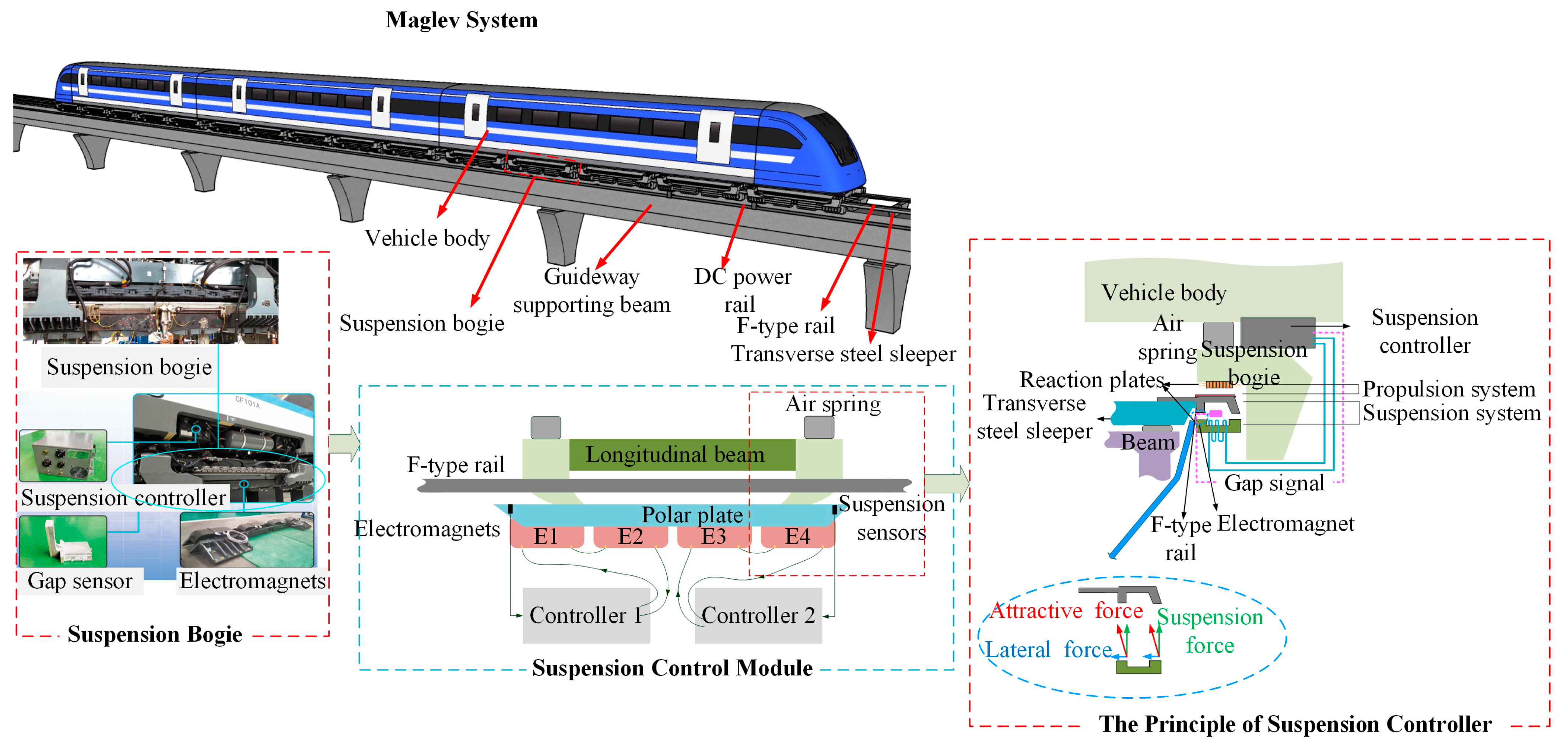
2. Overview of Maglev System

A common maglev system, as shown in Figure 1, is composed of an elevated guideway, a power rail, and an EMS-type train. The elevated guideway consists of the guideway supporting beam, a track bearing platform, fasteners, transverse steel sleepers, and an F-type rail. Each maglev vehicle typically has five bogies which work together to bear the weight of the vehicle body by using air springs as buffers and supporters. Each bogie is designed to couple two integrated electromagnets by using two suspension control modules on each side of the track. In general, a suspension control module consists of an integrated electromagnet panel (with four electromagnets clipped by a pair of integrated steel magnetic pole), two suspension sensors (including gap, current, and acceleration sensors) configured at each terminal of the integrated electromagnet panel, and two suspension controllers. The electromagnets are partitioned into two groups, in which the two electromagnets in the front (or rear) of the integrated electromagnet panel are connected in series as a pair, and the current through each pair of electromagnets is controlled by a suspension controller. As illustrated in Figure 1, the suspension controller receives signals from the current transformer, suspension gap, and acceleration sensors. Then, the signals are amplified by power chopper and sent to suspension electromagnets. With a proper control algorithm, the suspension electromagnets are commanded to generate an attractive force. The principal component of the attractive force is the suspension force, which enables the device to adjust the suspension gap and keep the suspension gap at a target, e.g., 8 mm. As the suspension gap reflects the distance between the electromagnets and the track, excessive fluctuation of the gap signal can directly lead to a fluctuation of the attractive force, resulting in the abnormal vibration of the track. In view of this, acceleration singles acquired by the track-side sensory system will be used for the real-time detection of potential malfunctions in the suspension control system.

3. Track-Side Online Monitoring System

The track-side online monitoring system for malfunction detection of the maglev suspension controllers is designed to meet the following requirements: (i) the deployed sensors, signal cables, and data acquisition unit are insulated to immunize them against electromagnetic interference (EMI); (ii) a sufficient signal acquisition resolution helping to single out malfunctioning suspension controllers; and (iii) an appropriate number of sensors to enable online malfunction detection while minimizing false alarms.

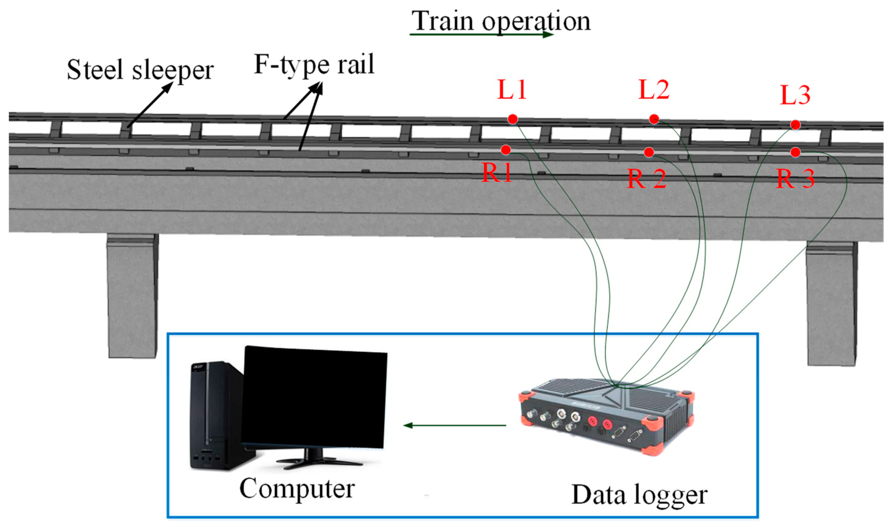
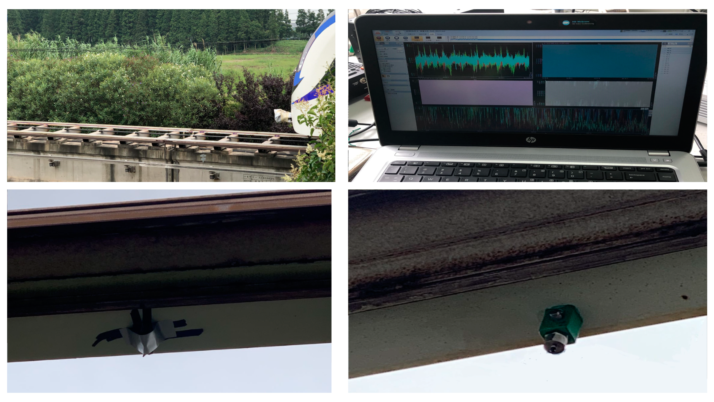
3.1. System Configuration

As illustrated in Figure 2, the proposed online monitoring system consists of the following: (i) two arrays of insulated piezoelectric accelerometers (or optic fiber accelerometers that are immune to EMI) deployed on the right and left F-type rails separately; (ii) a high-speed interrogator (data acquisition unit); and (iii) a computer equipped with data processing and fault identification software. To ensure a sufficiently high resolution, the monitoring system collects data at a sampling rate of 5000 Hz and is triggered to sample and store data automatically during the maglev train passage. To meet the demand for online execution, a BDLM-based method utilizing time-series data is developed for malfunction detection of the suspension control system. To minimize false alarms, each sensory array includes several accelerometers (e.g., three, as shown in Figure 2) located on each side of the F-type rail. The detailed deployment positions of the accelerometers will be provided in the next subsection.

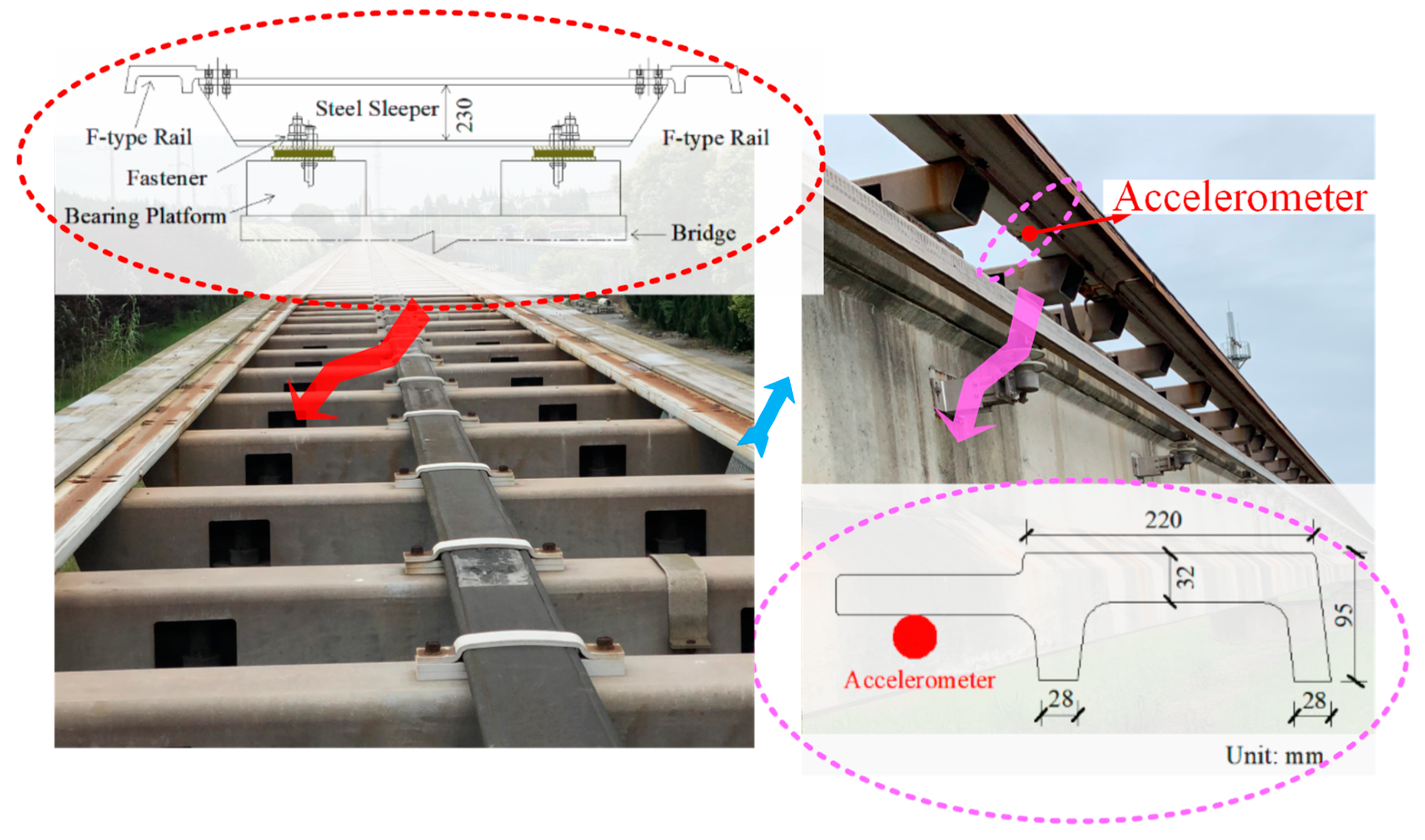
3.2. Deployment of Accelerometers

As the electromagnetic force between the electromagnets and the F-type rail is controlled by suspension controllers, and as each controller commands a pair of electromagnets, the paired electromagnets passing through the F-type rail cause an acceleration peak. If the paired electromagnets are controlled by a malfunctioning suspension controller, a distinct attractive force will be exerted on the F-type rail, resulting in abnormal response. As such, a set of accelerometers are mounted on a segment of the F-type rail to monitor the real-time dynamic response of the F-type rail and detect potential malfunction of the suspension controllers. Additionally, since the suspension force is the primary component of the attractive force (refer to Figure 1), the sensors are deployed on the F-type rail only for the measurement of accelerations in the vertical direction. As shown in Figure 3, the F-type rail is supported by the steel sleepers, and the accelerometers are mounted on the F-type rail between two adjacent steel sleepers. The cross section of the F-type rail is also shown in Figure 3, where the outward part of the F-type rail is named the inverted U-type orbit. The attractive force is generated between the U-type electromagnet and the inverted U-type orbit, as illustrated in Figure 1. Hence, the accelerometers are deployed at the cantilevered side (inward part) of the cross section of the F-type rail as shown in Figure 3. The deployed locations of sensors on the F-type rail are mid-span, 1/4 span, and end of the bridge. Each accelerometer measures the vertical vibration of the F-type rail excited by the suspension force.

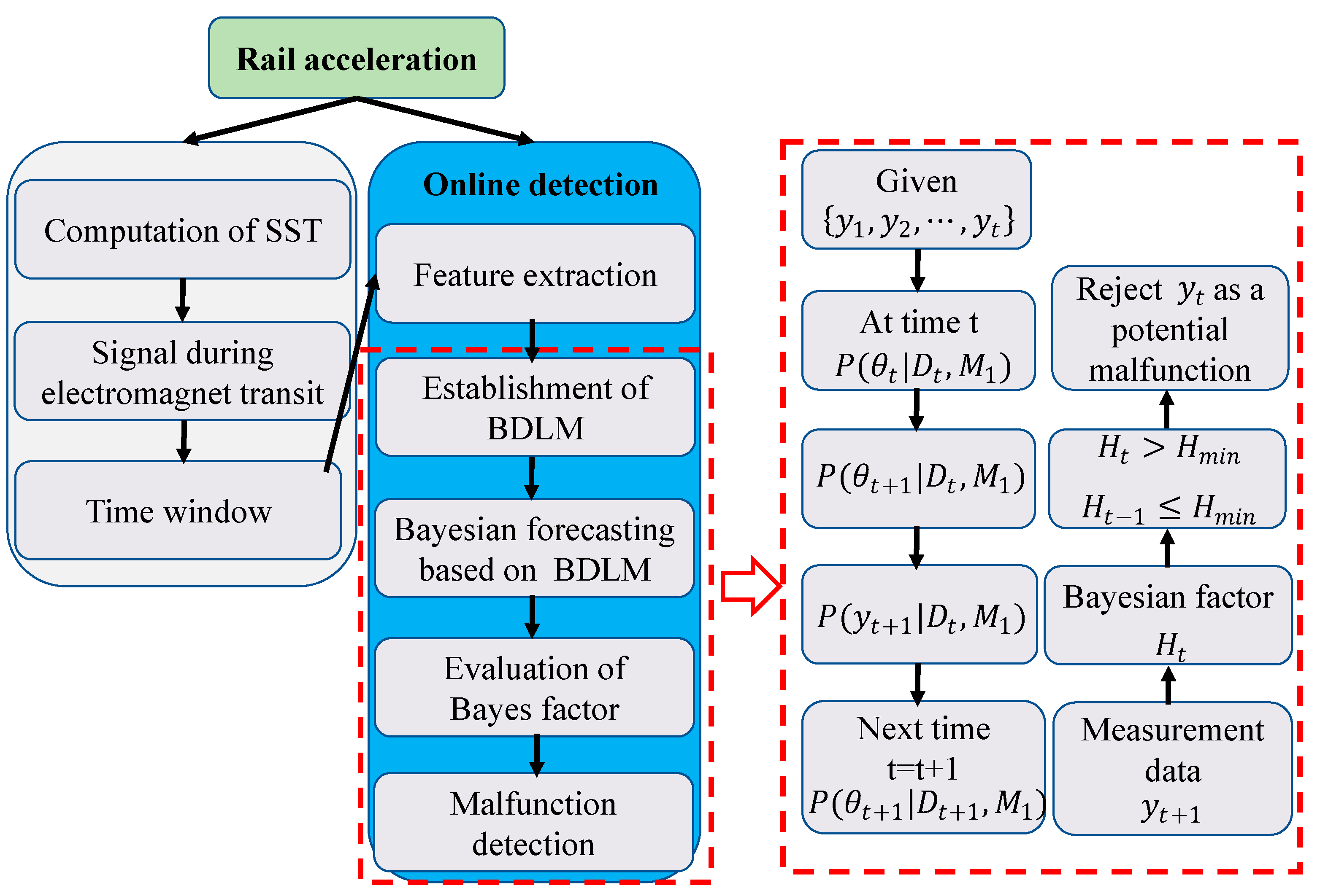
4. Track-Side Online Monitoring System Bayesian-Based Method for Online Malfunction Detection

4.1. General Description

In addition to the attractive force (controlled by suspension controllers) exerted on the F-type rail, each pair of integrated electromagnets also generates a moving magnetic force that acts on the rail when the paired electromagnets travel over it. The latter force results in a small-amplitude and low-frequency response ingredient in the rail, which will be extracted to identify the time interval (window) in conformance with the passage of each suspension controller. Due to its ability to extract individual components, the synchrosqueezing transform (SST) is performed for the extraction of this response ingredient from the raw acceleration signal. Then, the segmented acceleration signal stretching each time interval is adopted to construct the FI with modulation on the response amplitude, frequency, and train speed. The FI sequences are finally utilized to formulate BDLMs for detecting whether a specific suspension controller is malfunctioning or not.

4.2. Identification of Time Intervals during Electromagnet Transit

In order to link up the segmented acceleration responses with the respective suspension controllers, the SST is performed to extract the response ingredient caused by the moving magnetic force and estimate the time interval (window) of the acceleration signal during each electromagnet transit generated by a specific suspension controller. As a relatively new and promising signal processing tool based on the concepts of continuous wavelet transform (CWT), SST enables the decomposition of noisy nonstationary signals into their individual components. The signal with coarse resolution (approximations) contains information about low-frequency components, while the signal with fine resolution (details) contains information about high-frequency components. By using the wavelet-level selection and perfect reconstruction (PR) properties of SST for multi-component signal analysis, the response ingredient specifically caused by the moving magnetic force can be extracted from the raw acceleration signal. In the case of synchrosqueezing, as defined in [45], one starts from the CWT W x defined by
W x a , b = x t 1 a ψ t b a d t ,
where a is the scale parameter; b is the time parameter; and ψ · is the mother wavelet. The estimation of instantaneous frequency ω a , b for all values is given by [46]
ω a , b = i W x a ,   b b W x a , b .
In fact, the wavelet coefficients in W x a , b are computed only at discrete scales a k , and its synchrosqueezed counterpart T x ω c , b , determined at the centers ω c of the successive bins, can be derived as follows:
T x ω c , b = 1 Δ ω a k : ω a k , b ω c Δ ω / 2 W x a k , b a k 3 / 2 Δ a k ,
where Δ ω = ω c ω c 1 and Δ a = a k a k 1 . To reconstruct the signal after the synchrosqueezing, the following equation is defined as follows:
0 W x a , b a k 3 2 d a = 1 2 π 0 x ^ ξ ψ ^ a ξ e i b ξ a 1 d a d ξ = 0 ψ ^ ξ d ξ ξ · 1 2 π 0 x ^ ζ e i b ζ d ζ .
Setting   C ψ = 1 2 0 ψ ^ ξ d ξ ξ , the individual modes can be recovered by inverting the SST (integrating) along the frequency axis as follows:
x c b = R e C ψ 1 c T x ω c , b Δ ω .
To obtain the response ingredient caused by the moving magnetic force, the low-frequency content is extracted from the raw signal. At the present sampling frequency, the low frequencies ranging from 1 Hz to 15 Hz are composed to generate the response caused by the moving magnetic force. As shown in the bottom panel of Figure 4, each response peak corresponds to the passage of a pair of integrated electromagnets (controlled by the suspension controller) over the rail, and the time interval (window) during each electromagnet transit driven by a specific suspension controller can be readily estimated from the noise-removed response curve.

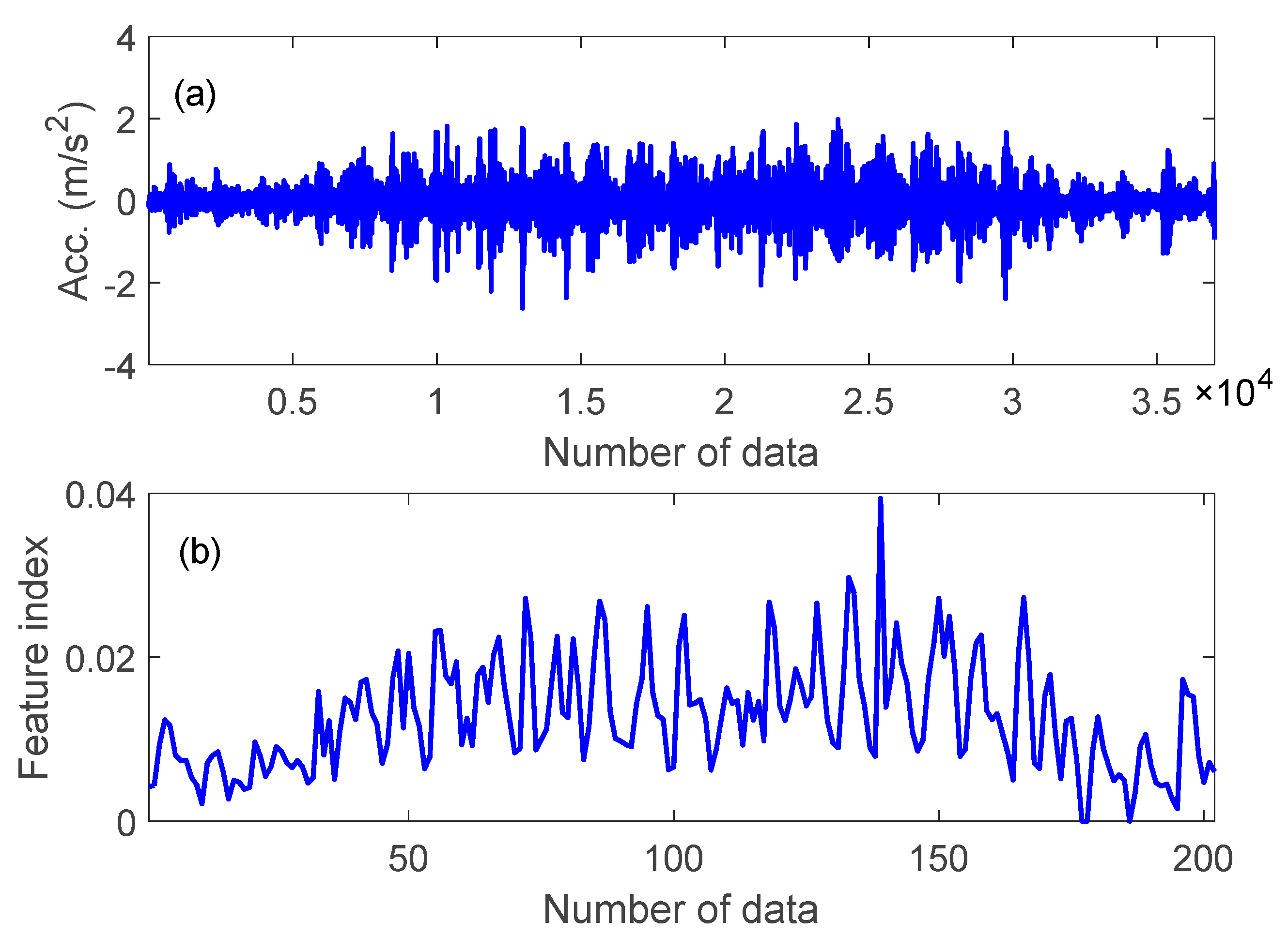
4.3. Feature Index (FI)

Figure 5 shows the acceleration responses and the power spectral densities of the F-type rail during electromagnet transit driven by different suspension controllers at two running speeds (30 km/h and 50 km/h). By analyzing and comparing large amounts of acceleration responses of the F-type rail under various running speeds and control statuses in both time and frequency domains, it is observed that the train’s running speed, vibration frequency, and vibration magnitude are the main factors which affect the response characteristics. For example, the acceleration response amplitude of the F-type rail increases in general with the increase in the running speed. The dominant vibration frequency of the F-type rail at the running speed of 30 km/h fluctuates between 39 Hz and 117 Hz, while the dominant vibration frequency of the F-type rail at the running speed of 50 km/h varies between 39 Hz and 156 Hz. To eliminate the influence of these normal variabilities on fault detection, we define the following feature index (FI):
χ i a n : n + m = f f c · 1 m j = n n + m a j 2 V ,
where χ i is the ith FI calculated from the acceleration response segment a n : n + m ; a n : n + m denotes the acceleration response segment from a n to a n + m , with n = 1 + (i- − 1) × (m- − p) being the start point; m is the length of acceleration response segment which equals the time interval (window) determined in the preceding subsection; p is the overlap length in calculating FI by using a moving time window scheme; f is the dominant frequency of the acceleration response segment a n : n + m ; fc is the minimum dominant frequency of the rail acceleration response (set to be 39 Hz in this study as it is the first-order vertical bending frequency of F-type rail); and V represents the train’s running speed.
With the time intervals determined by the SST method, the segmented acceleration responses of the F-type rail obtained at each sensor location can be used to calculate an FI sequence with the help of (6) (in this study, an overlap ratio of 50% is considered in time window moving). Figure 6 illustrates the acceleration response signal and the corresponding FI sequence obtained at one sensor location.

4.4. BDLM for Malfunction Detection

The BDLM consists of an observation (measurement) equation and a system (evolution) equation. The observation equation represents the relationship between the observed data and the unknown state parameters, while the system equation describes the evolution of state parameters over time. The two equations stated above are defined as follows [42]:
Observation   Equation :   y t = F t θ t + v t ,   v t ~ N 0 , V t
System   Equation :   θ t = G t θ t 1 + ω t ,   ω t ~ N 0 , W t ,
where y t is the observation vector at time t ; θ t is unknown state parameter vector; F t and G t are the respective known regression and evolution matrices; and v t and ω t are two independent Gaussian random vectors with mean zero and unknown covariance matrices V t and W t . The BDLM defined above amounts to treating θ t as a Markov chain, with y t being conditionally independent of θ t .
When applying BDLM to describe a time series, the observation is obtained by combining several elementary components, each of which captures a series of diverse features, such as trend, seasonality, and dependence on covariates [44]. To represent the trend in BDLM, the second order polynomial is considered in this study. The general expression of the second order polynomial BDLM is as follows [34]:
y t = μ t + v t ,   v t ~ N 0 , σ o b s 2
μ t = μ t 1 + α t 1 + ω 1 t ,   ω 1 t ~ N 0 , σ l e v e l 2
α t = α t 1 + ω 2 t ,   ω 2 t ~ N 0 , σ t r e n d 2 ,
where y t is the monitoring-derived time series data defined in (6); μ t represents the data range level at time t; α t represents the data range change between times t 1 and t; v t is a zero-mean Gaussian random variable representing the measurement error at moment t; and ω 1 t and ω 2 t are both zero-mean Gaussian random variables representing the evolution of BDLM from t 1 to t. In association with the standard BDLM defined in (7) and (8), we have the following:
θ t = μ t α t ,   F t = 1 0 ,   G t = 1 1 0 1 ,   W t = σ l e v e l 2 0 0 σ t r e n d 2 ,   V t = σ o b s 2 .
The details of utilizing BDLM for recursive one-step ahead forecast (posterior) of the distribution of the monitoring-derived time series data and fault detection under the Bayesian framework are presented as follows.
Step 1: Given the initial information D 0 , the distribution of initial state parameters characterizing the monitoring-derived time series data is specified as follows:
P ( θ 0 | D 0 ) ~ N m 0 , C 0 ,
where m 0 and C 0 are initial mean and variance of the state parameters, which can be determined by using the first measured data of the time series. Set t = 0 .
Step 2: By using the posterior distribution of the state parameters at current time t, P ( θ t | D t ) ~ N m t , C t , the prior distribution of the state parameters at next time t +1, P θ t + 1 | D t ~ N a t + 1 , R t + 1 , can be estimated by
a t + 1 = E θ t + 1 | D t = G t + 1 m t
R t + 1 = V a r θ t + 1 | D t = G t + 1 C t G t + 1 + W t + 1 ,
where D t is the state of information at time t ; and W t + 1 is the variance of the evolution error in the system equation.
Step 3: The mean and variance of the distribution of the data at next time t + 1 , P ( y t + 1 | D t )   ~ N f t + 1 , Q t + 1 , can be forecasted through the observation equation:
f t + 1 = E y t + 1 | D t = F t + 1 a t + 1
Q t + 1 = V a r y t + 1 | D t = F t + 1 R t + 1 F t + 1 + V t + 1 .
Step 4: Once the new data y t + 1 at time t + 1 is available, the posterior distribution of the state parameters can be updated to P ( θ t + 1 | D t + 1 ) ~ N m t + 1 , C t + 1 , of which the mean and variance are given by
m t + 1 = a t + 1 + A t + 1 e t + 1 ,   C t + 1 = R t + 1 A t + 1 A t + 1 T Q t + 1
e t + 1 = y t + 1 f t + 1 ,   A t + 1 = R t + 1 F t + 1 / Q t + 1 ,
where D t + 1 = D t , y t + 1 .
Step 5: The BDLM yields a PDF for the next measurement, labeled as M 0 . Meanwhile, an artificial alternative model, labeled as M 1 , is defined by shifting the mean of M 0 by +h. Thus, for each time step t , the Bayes factor is obtained as the ratio of the PDF under M 1 to that under M 0 [43], which can be calculated by
H t = p y t | D t 1 , M 1 p y t | D t 1 , M 0 ,
where y t is the measurement at time t ; and D t 1 refers to the history information up to time t 1 . In the case of Gaussian distributions, the Bayes factor is as follows:
H   t = exp ± 2 h y t f t h 2 2 σ t 2 ,
where ± represents the positive deviation value and the negative deviation value, respectively; and h is the shift value, which can be determined by the inverse of the standard normal cumulative distribution function 1 , the confidence level α , and the standard deviation for the forecasting σ t as follows:
h = 1 1 α 2 σ t
Step 6: Set t = t + 1 and repeat the steps from Step 2 until to the end of the observation data.
To summarize the steps of using BDLM for recursive one-step ahead forecast (posterior) of the distribution of the monitoring-derived time series data and fault detection under the Bayesian framework, the pseudocode of Bayesian probability recursive processes of BDLM is given in Table 1.
Potential malfunction detection is a crucial step in the process of the proposed malfunction detection approach, accomplished by the Bayes factor calculation. Because of its straightforward and natural interpretation of the evidence afforded by the data, Bayes factor is advocated in fault detection [40]. In general, a Bayes factor H = 1 indicates that the probability of the observation derived from model M1 is identical to the probability of that derived from model M0. For better quantitative comparison between any two models, Jeffreys [47] suggested interpreting the Bayes factor as a scale of evidence and provided descriptive statements, although the partitions are somewhat arbitrary. According to his suggestion, a Bayes factor is divided into several intervals for assessing the significance of discrimination: 1 < H < 3 is ‘barely worth mentioning’; 3 < H < 10 is ‘substantial’, 10 < H < 30 is ‘strong’; 30 < H < 100 is ‘very strong’; and H > 100 is ‘decisive’. In this study, H m i n = 10 is set as a threshold for malfunction detection. With this threshold and a confidence level of 90% adopted, the shift value h is obtained as 1.645 σ t . After the confirmation of Hmin and h, an uncertainty limit ( u c l = ln H m i n h σ t 2 + h / 2 ) can be procured as 2.22 σ t . Thus, an observation is diagnosed as a malfunction if its deviation from the mean value of M0 is larger than 2.22 σ t . The flowchart of the malfunction detection framework based on BDLM is shown in Figure 7.

5. In-Suit Verification

5.1. Full-Scale Tests

For the purpose of verification, the online monitoring system has been deployed on a maglev test line and acceleration responses of the instrumented F-type rail have been collected during the trial run of a maglev train with malfunctions in its suspension control system being artificially introduced (the running speed was controlled and did not exceed 50 km/h to ensure the operation safety). The maglev test line and the deployed sensors are shown in Figure 8, where three accelerometers were installed on each side of a segment of the F-type rail supported by a viaduct (refer to Figure 2). The maglev train in the trial run comprises three vehicles, and each maglev vehicle has five bogies and twenty suspension controllers. The suspension gap between the electromagnets and the F-type rail is targeted to be 8 mm. When the maglev train travels through a straight guideway, the allowable variation of the suspension gap is limited to ±2 mm. As the performance of the suspension gap signal filters can directly influence the working condition of the suspension controllers, the artificial malfunction was made on two controllers of the maglev train by improperly altering the filter parameters, whereas the controllers with malfunctions were unknown to us at the test stage. The accelerations of the F-type rail were recorded as the train traveled over the instrumented rail at different running speeds. In the meantime, the signals of the suspension sensors were also stored in the controller area network (CAN) system of the maglev train at a low sampling rate of 4.0 Hz, which will be utilized to examine the fidelity of malfunctioning controllers identified by the proposed method.
In the following, the malfunction detection results using the accelerations obtained at different sensor locations and under different running speeds will be presented and discussed. In particular, the results obtained using the modulated FI sequences and using the raw acceleration data will be compared. Afterwards, the gap signals collected by the suspension sensors will be provided to verify the malfunction detection results.

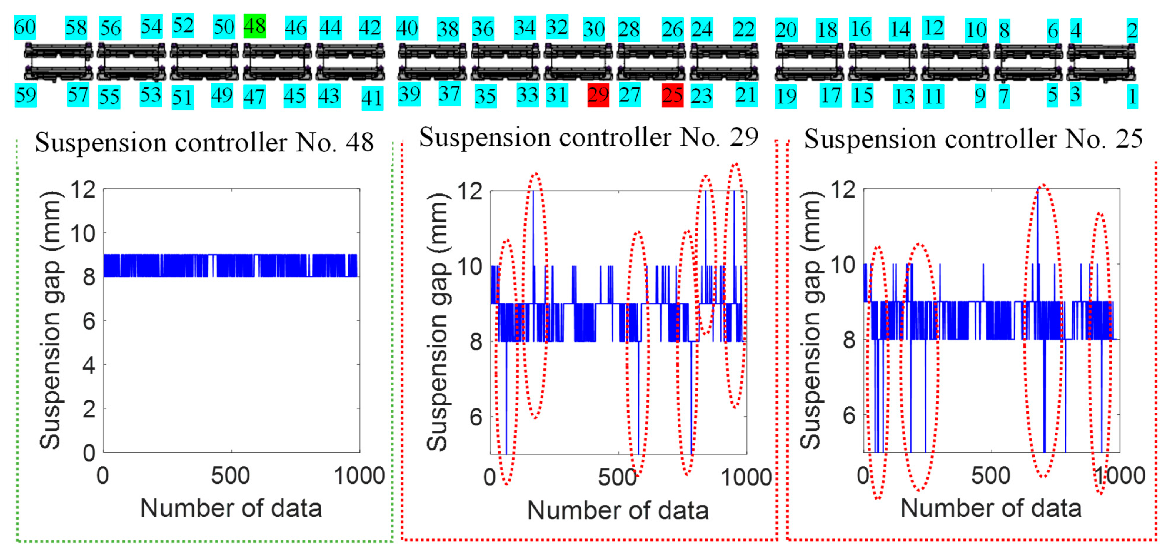
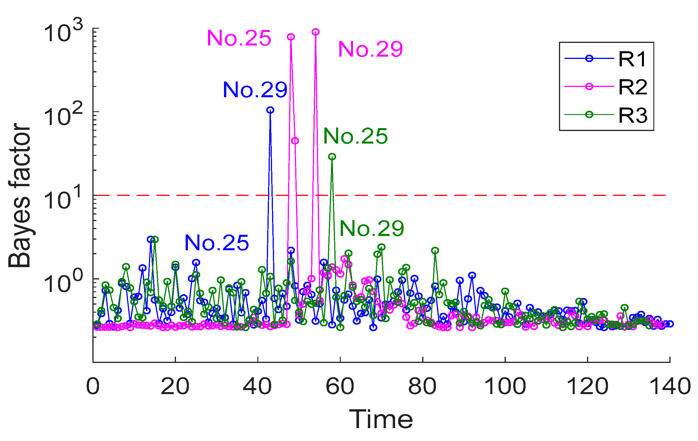
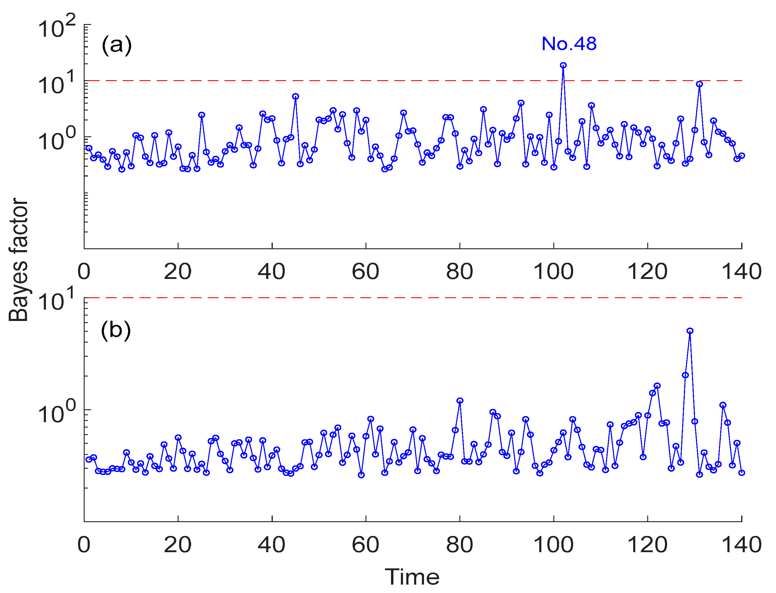
5.2. Malfunction Detection Results by Using Accelerations at Different Locations

As illustrated in Figure 2, accelerometers are deployed at three locations on each side of the F-type rail. The accelerations at locations R1, R2, R3, and L4 obtained under the running speed of 50 km/h are used here to illustrate the malfunction detection capability of the BDLM-based method in line with the FI sequences. Figure 9 illustrates the malfunction detection results of the suspension controllers. It is seen that the Bayes factor (H) at time points t = 38 and t = 43 in Figure 9 a exceeds the threshold value of Hmin = 10, indicating that suspension controllers corresponding to these two malfunctioning points are not in good performance. Meanwhile, it is observed that the Bayes factor at time points t = 48 and t = 53 in Figure 9b and at time points t = 58 and t = 63 in Figure 9c exceeds the threshold. More importantly, it is found that the time interval of the first malfunction point between Figure 9a,b is the same as that between Figure 9b,c. The same observation is obtained for the second malfunction point. Therefore, making use of the acceleration measurements at three locations, the malfunctioning suspension controllers can be reliably detected with mutually verifiable results. With the identified malfunction points, the two controllers with malfunctions are consistently identified to be suspension controllers No. 25 and No. 29. The suspension gap signals of suspension controllers No. 25 and No. 29 are illustrated in Figure 10 (the gap signals look discontinuous because they were acquired at a low sampling rate via built-in equipment). It is evidenced that the gap fluctuations at suspension controllers No. 25 and No. 29 are up to +4 mm and −3 mm, respectively, exceeding the maximum allowable variation of ±2 mm.
To verify the effectiveness of the formulated FI, malfunction detection is also conducted by applying the BDLM-based method but using the raw acceleration data directly. The results are illustrated in Figure 11. It is seen that the two malfunctioning suspension controllers are correctly detected using the acceleration collected at R2, but only one malfunctioning suspension controller is detected using the acceleration collected at R1 and R3. Likewise, the acceleration signal collected at L1 is also used to identify potential malfunctioning suspension controller(s) above the left rail, using of the raw acceleration data and the FI sequence, respectively. The detection results are illustrated in Figure 12. It is seen that one suspension controller (No. 48) is identified as malfunctioning when using the raw acceleration data (Figure 12a), but no malfunctioning suspension controller is detected when using the FI sequence (Figure 12b). The gap signal of suspension controller No. 48 is shown in Figure 10. As can be observed from Figure 10, the condition of the suspension controller No. 48 is healthy. This implies that this suspension controller is falsely identified as malfunctioning when using the raw acceleration signal instead of the FI sequence.

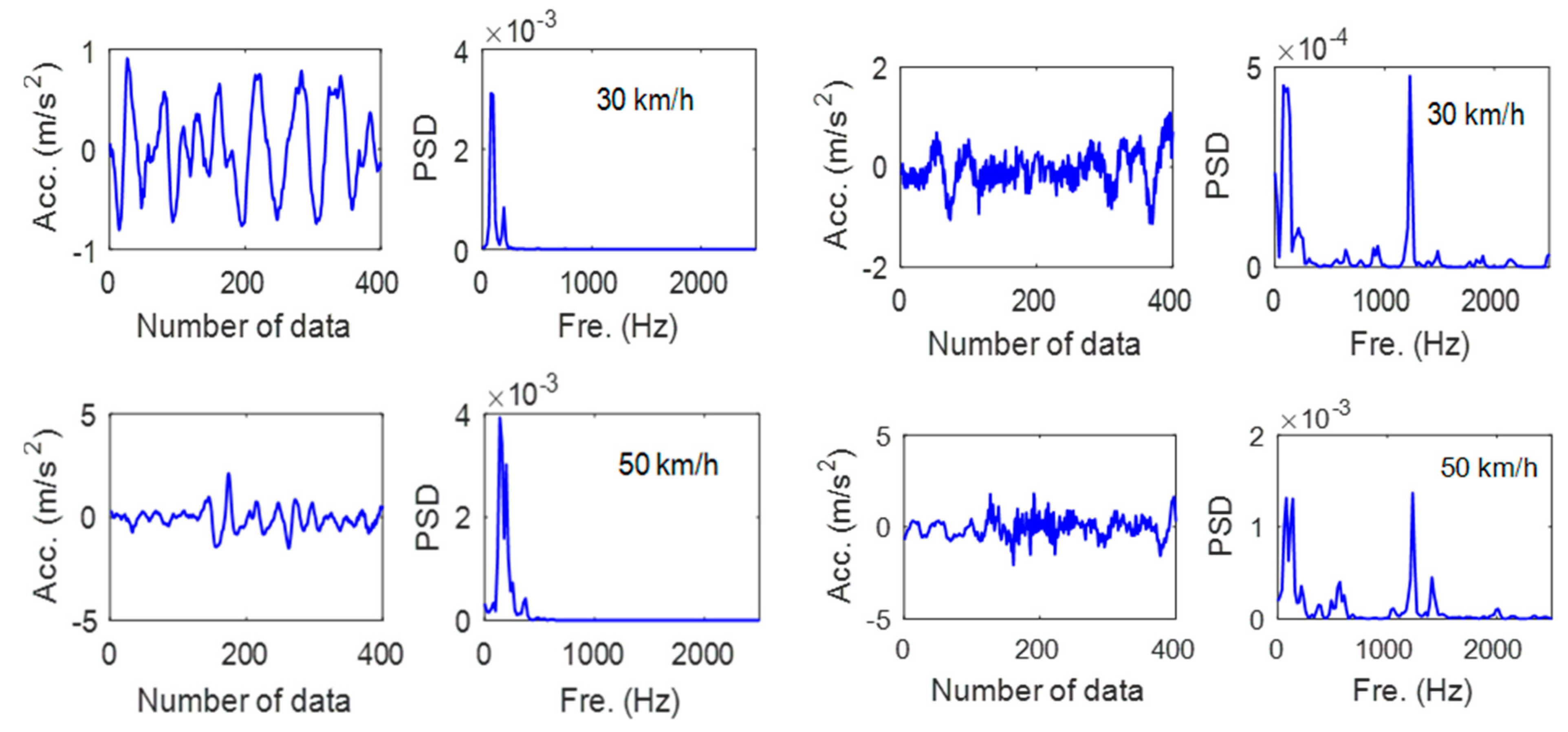
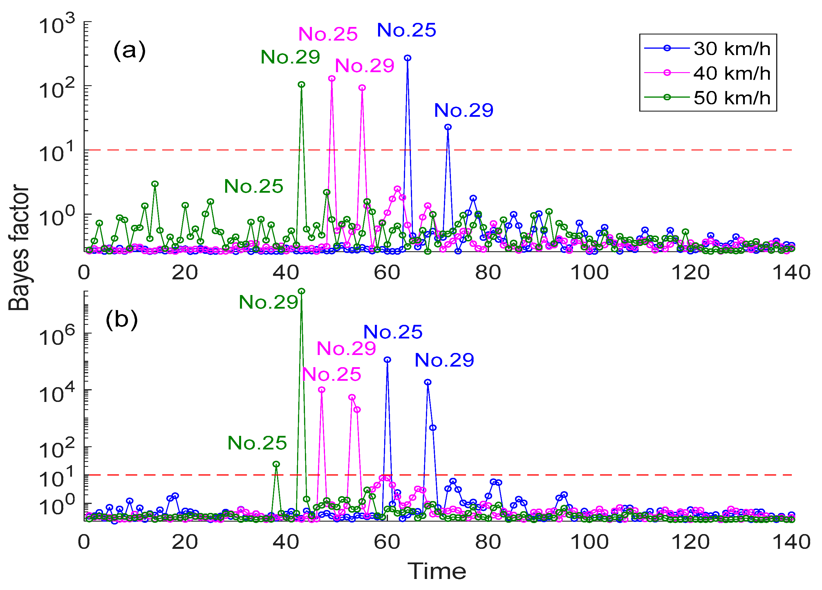
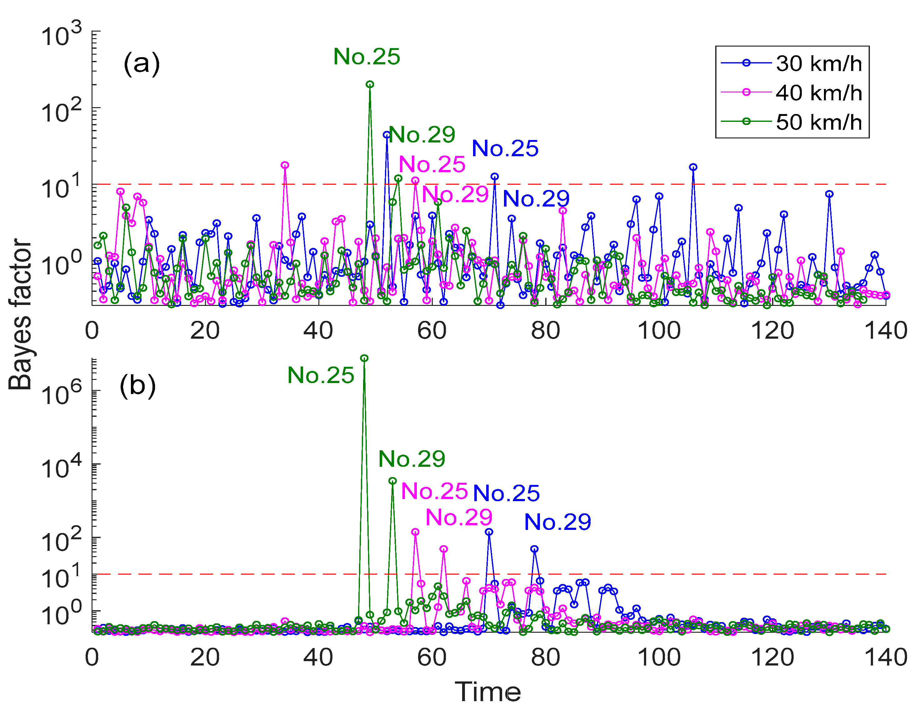
5.3. Malfunction Detection Results by Using Accelerations at Different Running Speeds

As the vibration of the F-type rail is also affected by the running speed of the train, the FI was modulated by the running speed in its formulation. Now, we examine the fidelity of the malfunction detection results obtained under different running speeds. During the trial run of the maglev train, acceleration response signals of the F-type rail were collected at three running speeds: 30 km/h, 40 km/h, and 50 km/h. By utilizing the raw acceleration signals and the derived FI sequences at the three running speeds, respectively, the Bayesian factor is elicited for malfunction detection of the suspension controllers. Figure 13 shows the detection results when using the accelerations collected at location R1 under different running speeds. It is observed from Figure 13b that when using the FI sequence in the BDLM-based method, the Bayesian factor exceeds the threshold value (Hmin = 10) at time points t = 60 and t = 68 for running speed of 30 km/h, at time points t = 47 and t = 53 for running speed of 40 km/h, and at time points t = 38 and t = 43 for running speed of 50 km/h, which all indicate the identical malfunctioning suspension controllers (No. 25 and No. 29). This means that the proposed method yields correct and consistent malfunction detection results when using the FI sequences formulated from accelerations obtained under different running speeds. However, as shown in Figure 13a, when the raw acceleration signals are used for malfunction detection, the Bayesian factor exceeds the threshold at time points t = 60 and t = 68 for 30 km/h, at time points t = 47 and t = 53 for 40 km/h, and at time point t = 43 only for 50 km/h. It is shown that using the raw acceleration signals enables the detection both malfunctioning controllers at running speeds of 30 km/h and 40 km/h, but the malfunctioning controller No. 25 is not identified at the running speed of 50 km/h. Similar results are obtained when using accelerations collected at locations R2 and R3, as shown in Figure 14 and Figure 15. In summary, the malfunctioning suspension controllers can be detected with high fidelity when using the FI sequences formulated from accelerations acquired at different locations and under different running speeds. However, when directly using the raw acceleration signals without modulation, either false-negative (refer to Figure 13a, Figure 14a and Figure 15a) or false-positive (refer to Figure 14a and Figure 15a) detection results can be yielded.
The BDLM-based method is performed on a Lenovo ThinkCentre M720t desktop (Lenovo, Beijing, China) with Dual Intel Core i7-8700 processor (Intel, CA, USA) and 24 GB of memory. The average computation time of the BDLM-based method is 2.23 s. As the BDLM-based method can automatically detect the malfunction of the suspension controller, real-time malfunction detection can be realized using the BDLM-based method.

6. Conclusions

A track-side online monitoring system in conjunction with the Bayesian dynamic model has been developed for malfunction detection in the suspension system of maglev trains during their routine operation. The system, which consists of accelerometers deployed on both sides of a segment or a few segments of the F-type rail, aims to detect potential malfunction in all suspension controllers affiliated with a maglev train when it travels over the instrumented rail. By means of the synchrosqueezing transform (SST), the time interval (window) of rail acceleration responses in conformance with the electromagnet transit generated by each passing suspension controller is first identified in order to correlate each time interval with a specific suspension controller. Then, a feature index (FI) is formulated from the monitored acceleration responses after modulating the response amplitude, frequency, and train’s running speed. The derived FI sequence is used to construct a Bayesian dynamic linear model (BDLM) and elicit Bayes factor for malfunction detection in suspension controllers.
The capability of the proposed monitoring system and malfunction detection algorithm was exemplified by using rail accelerations collected during a trial run of a maglev train on a test line where the devised monitoring system was installed. In the field tests, malfunction of the suspension controllers was artificially introduced by improperly altering the parameters of a few suspension gap signal filters, and the gap signals were collected and stored by built-in equipment for verification of the detection results via the proposed method. The field test results confirm the following: (i) with the use of rail acceleration measurements at multiple locations, suspension controllers with malfunction can be reliably identified with mutually verifiable results via the proposed BDLM-based method in line with the FI sequence; (ii) when directly using the raw acceleration signal to formulate BDLM, either false-negative or false-positive detection results can be generated; and (iii) in comparison with the BDLM famulated using the raw acceleration signal, the BDLM famulated using the FI sequence is more robust and tolerant with respect to the running speed and sensor location.
As the proposed online monitoring system consists of only two arrays of insulated piezoelectric accelerometers, a high-speed interrogator and a computer equipped with data processing and fault identification software, the cost of the proposed technology depends on the price of equipment which is relatively low. In the future, the accuracy and efficiency of the proposed algorithm under different operation conditions, such as those introducing wind, vehicle loading changes, and higher train speed, will be further studied.

Author Contributions

Conceptualization, Y.-Q.N.; methodology, S.-M.W.; software, Y.-W.W.; validation, S.-M.W., Y.-W.W., and Y.-Q.N.; data curation, Y.L.; writing—original draft preparation, S.-M.W.; writing—review and editing, Y.-Q.N. All authors have read and agreed to the published version of the manuscript.

Funding

This research was funded by the National Natural Science Foundation of China (project No. U1934209); by Wuyi University’s Hong Kong and Macao Joint Research and Development Fund (project No. 2019WGALH15, 2019WGALH17, and 2021WGALH15); by the Innovation and Technology Commission of Hong Kong SAR Government (project No. K-BBY1); and by the Hong Kong Polytechnic University (PolyU) Start-up Fund for RAPs under the Strategic Hiring Scheme (project No. P0039260).

Data Availability Statement

Not applicable.

Conflicts of Interest

The authors declare no conflict of interest.

References

  1. Long, Z.; Xue, S.; Zhang, Z.; Xie, Y. A new strategy of active fault-tolerant control for suspension system of maglev train. In Proceedings of the 2007 IEEE International Conference on Automation and Logistics, Jinan, China, 18–21 August 2007; pp. 88–94. [Google Scholar]
  2. Ono, M.; Koga, S.; Ohtsuki, H. Japan’s superconducting maglev train. IEEE Instrum. Meas. Mag. 2002, 5, 9–15. [Google Scholar] [CrossRef]
  3. Huang, C.M.; Yen, J.Y.; Chen, M.S. Adaptive nonlinear control of repulsive maglev suspension systems. Control Eng. Pract. 2000, 8, 1357–1367. [Google Scholar] [CrossRef]
  4. Li, Y.; Li, J.; Zhang, G.; Tian, W.J. Disturbance decoupled fault diagnosis for sensor fault of maglev suspension system. J. Cent. South Univ. 2013, 20, 1545–1551. [Google Scholar] [CrossRef]
  5. Zhou, D.; Li, J.; Hansen, C.H. Suppression of the stationary maglev vehicle-bridge coupled resonance using a tuned mass damper. J. Vib. Control 2013, 19, 191–203. [Google Scholar] [CrossRef]
  6. Li, J.; Li, J.; Zhou, D.; Cui, P.; Wang, L.; Yu, P. The active control of maglev stationary self-excited vibration with a virtual energy harvester. IEEE Trans. Ind. Electron. 2014, 62, 2942–2951. [Google Scholar] [CrossRef]
  7. Wai, R.J.; Lee, J.D. Adaptive fuzzy-neural-network control for maglev transportation system. IEEE Trans. Neural Netw. 2008, 19, 54–70. [Google Scholar] [PubMed]
  8. Zhou, D.; Li, J.; Zhang, K. Amplitude control of the track-induced self-excited vibration for a maglev system. ISA Trans. 2014, 53, 1463–1469. [Google Scholar] [CrossRef]
  9. Xu, Y.L.; Wang, Z.L.; Li, G.Q.; Chen, S.; Yang, Y.B. High-speed running maglev trains interacting with elastic transitional viaducts. Eng. Struct. 2019, 183, 562–578. [Google Scholar] [CrossRef]
  10. Wang, Z.L.; Xu, Y.L.; Li, G.Q.; Yang, Y.B.; Chen, S.W.; Zhang, X.L. Modelling and validation of coupled high-speed maglev train-and-viaduct systems considering support flexibility. Veh. Syst. Dyn. 2019, 57, 161–191. [Google Scholar] [CrossRef]
  11. Xu, J.; Zhou, Y. A nonlinear control method for the electromagnetic suspension system of the maglev train. J. Mod. Transp. 2011, 19, 176–180. [Google Scholar] [CrossRef]
  12. Wang, P.; Long, Z.; Dang, N. Multi-model switching based fault detection for the suspension system of maglev train. IEEE Access 2018, 7, 6831–6841. [Google Scholar] [CrossRef]
  13. Wang, L.; Yu, P.; Li, J.; Zhou, D.; Li, J. Suspension system status detection of maglev train based on machine learning using levitation sensors. In Proceedings of the 2017 29th Chinese Control and Decision Conference, Chongqing, China, 28–30 May 2017; pp. 7579–7584. [Google Scholar]
  14. Long, Z.Q.; Chen, X.Y.; Fan, C.X. Middle-low speed maglev train suspension control system common cause failure risk analysis. In Proceedings of the 2017 36th Chinese Control Conference, Dalian, China, 26–28 July 2017; pp. 7218–7224. [Google Scholar]
  15. Sun, Y.; Xu, J.; Qiang, H.; Chen, C.; Lin, G.B. Adaptive sliding mode control of maglev system based on RBF neural network minimum parameter learning method. Measurement 2019, 141, 217–226. [Google Scholar] [CrossRef]
  16. Zhou, D.; Yu, P.; Wang, L.; Li, J. An adaptive vibration control method to suppress the vibration of the maglev train caused by track irregularities. J. Sound Vib. 2017, 408, 331–350. [Google Scholar] [CrossRef]
  17. Hou, Z.; Gan, W.; Xu, S.; Guo, W.; Chen, Q.; Wang, W.; Chen, K. Fault detection of accelerometer and fault-tolerant control for maglev. In Proceedings of the 2019 IEEE Vehicle Power and Propulsion Conference, Hanoi, Vietnam, 14–17 October 2019; pp. 1–5. [Google Scholar]
  18. Yin, S.; Rodriguez-Andina, J.J.; Jiang, Y. Real-time monitoring and control of industrial cyberphysical systems: With integrated plant-wide monitoring and control framework. IEEE Ind. Electron. Mag. 2019, 13, 38–47. [Google Scholar] [CrossRef]
  19. Wang, Y.W.; Ni, Y.Q.; Wang, S.M. Structural health monitoring of railway bridges using innovative sensing technologies and machine learning algorithms: A concise review. Intell. Transp. Infrastruct. 2022, 1, liac009. [Google Scholar] [CrossRef]
  20. Sun, Y.; Qiang, H.; Xu, J.; Lin, G. Internet of Things-based online condition monitor and improved adaptive fuzzy control for a medium-low-speed maglev train system. IEEE Trans. Ind. Inform. 2019, 16, 2629–2639. [Google Scholar] [CrossRef]
  21. Kang, D.; Chung, W. Integrated monitoring scheme for a maglev guideway using multiplexed FBG sensor arrays. NDT E Int. 2009, 42, 260–266. [Google Scholar] [CrossRef]
  22. He, Q.; Wang, J.; Hu, F.; Kong, F. Wayside acoustic diagnosis of defective train bearings based on signal resampling and information enhancement. J. Sound Vib. 2013, 332, 5635–5649. [Google Scholar] [CrossRef]
  23. Ngigi, R.W.; Pislaru, C.; Ball, A.; Gu, F. Modern techniques for condition monitoring of railway vehicle dynamics. J. Phys. Conf. Ser. 2012, 364, 012016. [Google Scholar] [CrossRef]
  24. Filograno, M.L.; Corredera, P.; Rodriguez-Plaza, M.; Andres-Alguacil, A.; Gonzalez-Herraez, M. Wheel flat detection in high-speed railway systems using fiber Bragg gratings. IEEE Sens. J. 2013, 13, 4808–4816. [Google Scholar] [CrossRef]
  25. Liu, X.Z.; Ni, Y.Q. Wheel tread defect detection for high-speed trains using FBG-based online monitoring techniques. Smart Struct. Syst. 2018, 21, 687–694. [Google Scholar]
  26. Wei, C.; Xin, Q.; Chung, W.H.; Liu, S.Y.; Tam, H.Y.; Ho, S.L. Real-time train wheel condition monitoring by fiber Bragg grating sensors. Int. J. Distrib. Sens. Netw. 2011, 8, 409048. [Google Scholar] [CrossRef]
  27. Han, H.S.; Kim, D.S. Magnetic Levitation: Maglev Technology and Applications; Springer: Dordrecht The Netherlands, 2016. [Google Scholar]
  28. Frank, P.M. Analytical and qualitative model-based fault diagnosis—A survey and some new results. Eur. J. Control 1996, 2, 6–28. [Google Scholar] [CrossRef]
  29. Gao, Z.; Cecati, C.; Ding, S.X. A survey of fault diagnosis and fault-tolerant techniques—Part I: Fault diagnosis with model-based and signal-based approaches. IEEE Trans. Ind. Electron. 2015, 62, 3757–3767. [Google Scholar] [CrossRef]
  30. Gao, Z.; Cecati, C.; Ding, S.X. A survey of fault diagnosis and fault-tolerant techniques—Part II: Fault diagnosis with knowledge-based and hybrid/active approaches. IEEE Trans. Ind. Electron. 2015, 62, 3768–3774. [Google Scholar] [CrossRef]
  31. Jiang, Y.; Yin, S.; Kaynak, O. Optimized design of parity relation-based residual generator for fault detection: Data-driven approaches. IEEE Trans. Ind. Inform. 2021, 17, 1449–1458. [Google Scholar] [CrossRef]
  32. Yin, S.; Ding, S.X.; Xie, X.; Luo, H. A review on basic data-driven approaches for industrial process monitoring. IEEE Trans. Ind. Electron. 2014, 61, 6418–6428. [Google Scholar] [CrossRef]
  33. Zang, Y.; Shang, G.W.; Cai, B.; Wang, H.; Pecht, M.G. Methods for fault diagnosis of high-speed railways: A review. Proc. Inst. Mech. Eng. Part O J. Risk Reliab. 2019, 233, 908–922. [Google Scholar] [CrossRef]
  34. Chen, H.; Jiang, B.; Ding, S.X.; Huang, B. Data-driven fault diagnosis for traction systems in high-speed trains: A survey, challenges, and perspectives. IEEE Trans. Intell. Transp. Syst. 2020, 23, 1700–1716. [Google Scholar] [CrossRef]
  35. Chen, H.; Jiang, B.; Ding, S.X. A broad learning aided data-driven framework of fast fault diagnosis for high-speed trains. IEEE Intell. Transp. Syst. Mag. 2020, 13, 83–88. [Google Scholar] [CrossRef]
  36. Davari, N.; Veloso, B.; Costa, G.D.A.; Pereira, P.M.; Ribeiro, R.P.; Gama, J. A survey on data-driven predictive maintenance for the railway industry. Sensors 2021, 21, 5739. [Google Scholar] [CrossRef]
  37. Wang, S.M.; Jiang, G.F.; Ni, Y.Q.; Lu, Y.; Lin, G.B.; Pan, H.L.; Xu, J.Q.; Hao, S. Multiple damage detection of maglev rail joints using time-frequency spectrogram and convolutional neural network. Smart Struct. Syst. 2022, 29, 625–640. [Google Scholar]
  38. Li, H.W.; Yang, D.S.; Sun, Y.L.; Han, J. Study review and prospect of intelligent fault diagnosis technique. Comput. Eng. Des. 2013, 34, 632–637. [Google Scholar]
  39. Ni, Y.Q.; Wang, Y.W.; Zhang, C. A Bayesian approach for condition assessment and damage alarm of bridge expansion joints using long-term structural health monitoring data. Eng. Struct. 2020, 212, 110520. [Google Scholar] [CrossRef]
  40. Wang, Y.W.; Ni, Y.Q.; Wang, X. Real-time defect detection of high-speed train wheels by using Bayesian forecasting and dynamic model. Mech. Syst. Signal Process. 2020, 139, 106654. [Google Scholar] [CrossRef]
  41. Vagnoli, M.; Remenyte-Prescott, R.; Andrews, J. A fuzzy-based Bayesian belief network approach for railway bridge condition monitoring and fault detection. In Proceedings of the 2017 ESREL Conference on Safety and Reliability—Theory and Application, Portoroz, Slovenia, 18–22 June 2017. [Google Scholar]
  42. West, M.; Harrison, J. Bayesian Forecasting and Dynamic Models; Chapman and Hall: New York, NY, USA, 2006. [Google Scholar]
  43. Lipowsky, H.; Staudacher, S.; Bauer, M.; Schmidt, K.J. Application of Bayesian forecasting to change detection and prognosis of gas turbine performance. J. Eng. Gas Turbines Power 2012, 134, 031602. [Google Scholar]
  44. Wang, Y.W.; Ni, Y.Q. Bayesian dynamic forecasting of structural strain response using structural health monitoring data. Struct. Control. Health Monit. 2020, 27, e2575. [Google Scholar] [CrossRef]
  45. Daubechies, I.; Lu, J.; Wu, H.T. Synchrosquee zed wavelet transforms: An empirical mode decomposition-like tool. Appl. Comput. Harmon. Anal. 2011, 30, 243–261. [Google Scholar] [CrossRef]
  46. Meignen, S.; Oberlin, T.; Pham, D.H. Synchrosqueezing transforms: From low-to high-frequency modulations and perspectives. Comptes Rendus Phys. 2019, 20, 449–460. [Google Scholar] [CrossRef]
  47. Jeffreys, H. Theory of Probability; Oxford Clarendon Press: Oxford, UK, 1961. [Google Scholar]
Figure 1. Configuration of maglev train system.
Mathematics 11 04045 g001
Figure 2. Configuration of the online monitoring system.
Mathematics 11 04045 g002
Figure 3. Deployment of accelerometers on the F-type rail.
Mathematics 11 04045 g003
Figure 4. Raw response signal and SST-extracted response ingredient caused by moving magnetic force and time window.
Mathematics 11 04045 g004
Figure 5. Accelerations of F-type rail driven by different suspension controllers and their power spectral densities under running speeds of 30 km/h and 50 km/h.
Mathematics 11 04045 g005
Figure 6. Acceleration response signal and feature index (FI) sequence: (a) raw acceleration response; (b) FI sequence.
Mathematics 11 04045 g006
Figure 7. Flowchart of malfunction detection framework based on BDLM.
Mathematics 11 04045 g007
Figure 8. Track-side online monitoring system deployed on a maglev test line.
Mathematics 11 04045 g008
Figure 9. Malfunction detection results using FI sequences: (a) location R1; (b) location R2; (c) location R3.
Mathematics 11 04045 g009
Figure 10. Suspension gap signals of suspension controllers No. 25, No. 29, and No. 48.
Mathematics 11 04045 g010
Figure 11. Multifunction detection results using raw acceleration data collected at locations R1, R2, and R3.
Mathematics 11 04045 g011
Figure 12. Multifunction detection results using acceleration data collected at location L1: (a) results from raw acceleration data; (b) results from the FI sequence.
Mathematics 11 04045 g012
Figure 13. Multifunction detection results using acceleration data collected at R1 under different running speeds: (a) results from raw acceleration data; (b) results from FI sequence.
Mathematics 11 04045 g013
Figure 14. Multifunction detection results by using acceleration data collected at R2 under different running speeds: (a) results from raw acceleration data; (b) results from FI sequence.
Mathematics 11 04045 g014
Figure 15. Multifunction detection results by using acceleration data collected at R3 under different running speeds: (a) results from raw acceleration data; (b) results from FI sequence.
Mathematics 11 04045 g015
Table 1. The pseudocode of the Bayesian probability recursive processes of BDLM.
For t = 1→T
Calculate P ( θ t + 1 | D t ) through (14) and (15)
Sample f t + 1   a n d   Q t + 1 from P ( θ t + 1 | D t )
Calculate y t + 1 through (8)
Update P ( θ t + 1 | D t + 1 ) by adding new data y t + 1 through (18) and (19)
Calculate H t through (20)
End
Disclaimer/Publisher’s Note: The statements, opinions and data contained in all publications are solely those of the individual author(s) and contributor(s) and not of MDPI and/or the editor(s). MDPI and/or the editor(s) disclaim responsibility for any injury to people or property resulting from any ideas, methods, instructions or products referred to in the content.

