Optimal Consumption and Robust Portfolio Choice for the 3/2 and 4/2 Stochastic Volatility Models

Abstract

This manuscript derives optimal consumption and investment strategies for risk-averse investors under the 4/2 stochastic volatility class of models. We work under an expected utility (EUT) framework and consider a Constant Relative Risk Aversion (CRRA) investor, who may also be ambiguity-averse. The corresponding Hamilton–Jacobi–Bellman (HJB) and HJB–Isaacs (HJBI) equations are solved in closed-form for a subset of the parametric space and under some restrictions on the portfolio setting, for complete markets. Conditions for proper changes of measure and well-defined solutions are provided. These are the first analytical solutions for the 4/2 stochastic volatility model and the embedded 3/2 model for the type of excess returns established in the literature. We numerically illustrate the differences between the 4/2 model and the embedded cases of the 1/2 model (Heston) as well as the 3/2 model under the same data, and for two main cases: risk-averse investor in a complete market with consumption, and ambiguity-averse investor in a complete market with no consumption. In general, the 4/2 and 1/2 models recommend similar levels of consumption and exposure, while the 3/2 leads to significantly different recommendations.

1. Introduction

Dating back to the 1980s, in the seminal work of [1] (Equations II.1–II.8), the excess return of a security, also known as its risk premium, has been prescribed as proportional to powers of the volatility. Specifically, three models were proposed, all presented in terms of the market price of risk (MPR) —that is, technically the ratio of the excess return and the volatility of the security. The first model, type I, assumed an MPR proportional to volatility (i.e., power $1/2$). This model implies that each risk factor earns a risk premium that is proportional to the variance of the factor’s return. The second and the third models (types II and III) postulate constant MPR (i.e., power 0 on variance) and constant excess return (i.e., power $-1/2$ on variance, inversely proportional to volatility), respectively. These models have been widely used in the literature; see [2,3,4] for examples involving stochastic volatility (SV), stochastic interest, and jumps.

The specification of MPRs play a very important role in expected utility portfolio optimization. In this context, ref. [5] solved the portfolio optimization problem for MPR of types I and II, in a setting of CRRA (power) utility, in an incomplete market with finite horizon for the Heston model (also known as the 1/2 model). Ref. [6] considered the optimal investment and consumption problem in an incomplete market for the 3/2 model of [7] with Epstein–Zin–Weil recursive utility and an infinite horizon, which implies a value function independent of time. In particular, the authors considered two forms of excess return —constant and linear in the variance (i.e., the MPRs of types I and III). Nevertheless, the exact solution is only available when the agent’s elasticity of intertemporal substitution is one with constant excess return (type III). For all other cases, the solutions are approximations.

Our paper presents the very first closed-form analysis for type I MPR on the recently proposed 4/2 model (see [8]) with a finite horizon, consumption, and complete markets. This leads, as a by-product, to the first analysis of type I MPR on the 3/2 model. We incorporate several ingredients of interest to practitioners in an EUT setting: complete markets (incomplete market solutions follow trivially from our setting), consumption and terminal wealth, and ambiguity aversion.

Two recent studies have been conducted on the 4/2 model under MPRs outside of the settings in [1], while excluding consumption in their analyses. First, ref. [9] explored the optimal investment problem for a risk-averse investor in both incomplete and complete market in the absence of consumption. The authors employed the same MPR for the 1/2 and 3/2 components —proportional to $\sqrt{v_t}$, the driver of variance. This means that the Heston component follows the type II MPR in [5], whereas the 3/2 component follows type I MPR in [6]. Second, the work of [10] considered an investor that is not only risk-averse, but also ambiguity-averse.

Solving the optimal consumption and asset allocation with the advanced 4/2 model for a type I MPR is challenging. The fact that our closed-form solutions are non-affine is proof of this challenge and an important departure from the exiting literature. When the MPR is proportional to a 4/2-structured volatility, the risk premium/excess return is proportional to the variance, ${\left(a\sqrt{v_t}+\frac{b}{\sqrt{v_t}}\right)}^2$. This means that there are nonlinear elements in the drift of the equity, which jeopardizes affine solutions and the solvability of the implied partial differential equations (PDEs) in the corresponding Hamilton–Jacobi–Bellman (HJB) and HJB Isaacs (HJBI) equations.

The contributions of our work are as follows:

• We conduct the first risk-averse, expected utility analysis in the presence of consumption for the non-affine class of SV models known as 4/2, under the preferable setting of MPR proportional to variance (type I). Our closed-form solutions, see Propositions 2, are of a non-affine nature, requiring confluent hypergeometric functions. As a by-product, we produce the very first closed-form portfolio analysis for the 3/2 model for finite horizons.
• We extend the solutions described above to an ambiguity-averse investor, leading to the very first related analyses for the 4/2 and 3/2 models, see Proposition 3. In all cases, we consider complete markets, providing conditions for well-defined solutions under the assumption of existence, and proper changes of measure.
• For a risk-averse investor, in a complete market, we illustrate the differences between the 4/2 model and the popular embedded cases of the 1/2 (Heston) and 3/2 models. On the one hand, the 4/2 and 1/2 models recommend similar levels of consumption and exposure. On the other hand, the 3/2 leads to 20% or higher levels of consumption and absolute exposures (see Figure 1, Figure 2, Figure 3, Figure 4, Figure 5 and Figure 6).
  The difference in terms of exposures is exacerbated when considering an ambiguity-averse investor in a complete market. In such case, the 3/2 model performance could double absolute exposures compared to the 1/2 and 4/2 models (see Section 5.1).

This paper contains five sections. Section 2 describes the 4/2 model under consideration and the derivatives needed in the portfolio. Section 3 presents and solves the consumption and terminal wealth expected utility problem for a risk-averse investor. Section 3.1 focuses on the complete market case. Section 4 then extends the problematic to an ambiguity-averse investor, with a section on complete markets (Section 4.1). Section 5 studies and implements the top three main cases numerically. First, Section 5.1 analyses a risk-averse investor in a complete market with consumption. Second, Section 5.2 studies an ambiguity-averse complete market investor with no consumption. Finally, Section 6 provides conclusions. All proofs are provided with details in a complementary Appendix A.

2. Description of the Model

The stochastic processes in the financial market are defined on a complete probability space $(\Omega ,\mathcal{F},\mathbb{P})$ with a right-continuous filtration ${\left\{{\mathcal{F}}_t\right\}}_{t\in [0,T]}$. The price process $S_t$ of the risky asset follows the 4/2 model described next:

$$\begin{array}{ccc}\hfill \frac{d{S}_t}{S_t}& =& \left(r+(\rho {\overline{\lambda }}_1+\sqrt{1-{\rho }^2}{\overline{\lambda }}_2){(a\sqrt{v_t}+\frac{b}{\sqrt{v_t}})}^2\right)dt+(a\sqrt{v_t}+\frac{b}{\sqrt{v_t}})d{W}_t,\hfill \end{array}$$

(1)

$$\begin{array}{ccc}\hfill d{v}_t& =& \kappa \left(\theta -v_t\right)dt+\sigma \sqrt{v_t}d{Z}_{1,t},v\left(0\right)=v_0>0,\hfill \end{array}\hspace{1em}\hspace{1em}\hspace{1em}\hspace{1em}\hspace{1em}\hspace{1em}\hspace{1em}\hspace{1em}\hspace{1em}\hspace{1em}\hspace{1em}\hspace{1em}$$

(2)

where $v_t$ drives the variance, and it follows a CIR with mean-reversion rate $\kappa >0$. The long-run mean is captured by $\theta >0$, and the volatility of volatility is denoted $\sigma >0$. The Feller condition (i.e., $2\kappa \theta \ge {\sigma }^2$) is imposed to ensure the process $v_t$ is strictly positive. The standard Brownian motions (BMs) $W_t$ in dynamic of risky asset $S_t$ and $Z_{1,t}$ in the dynamic of variance driver $v_t$ are correlated with parameter $\rho \in (-1,1)$. Thus, we will write $d{W}_t=\rho d{Z}_{1,t}+\sqrt{1-{\rho }^2}d{Z}_{2,t}$, where $Z_{2,t}$ is another standard BM, independent of $Z_{1,t}$. The variance, denoted by $z_t=z\left(v_t\right)$ is given as follows:

$$z_t={\left(a\sqrt{v_t}+\frac{b}{\sqrt{v_t}}\right)}^2=a^2{v}_t+\frac{b^2}{v_t}+2ab.$$

(3)

This setting implies market prices of risk with the following representation:

$$\left\{\begin{array}{cc}{\lambda }_1\left(v_t\right)\hfill & ={\overline{\lambda }}_1\left(a\sqrt{v_t}+\frac{b}{\sqrt{v_t}}\right),\hfill \\ {\lambda }_2\left(v_t\right)\hfill & ={\overline{\lambda }}_2\left(a\sqrt{v_t}+\frac{b}{\sqrt{v_t}}\right),\hfill \\ \lambda \left(v_t\right)\hfill & =\rho {\lambda }_1\left(v_t\right)+\sqrt{1-{\rho }^2}{\lambda }_2\left(v_t\right)=\overline{\lambda }\left(a\sqrt{v_t}+\frac{b}{\sqrt{v_t}}\right),\hfill \end{array}\right.$$

(4)

where $\overline{\lambda }=\left(\rho {\overline{\lambda }}_1+\sqrt{1-{\rho }^2}{\overline{\lambda }}_2\right)$, a and b are positive constants, ${\overline{\lambda }}_1$ and ${\overline{\lambda }}_2$ are constant. The process ${\lambda }_1\left(v_t\right)$ represents the market price of variance risk, and $\lambda \left(v_t\right)$ is the market price of stock risk. Moreover, ${\lambda }_2\left(v_t\right)$ can be understood as the market price of stock idiosyncratic risk (i.e., with respect to $Z_{2,t}$). Note that in this form of market price of risk, the excess return of the risky asset is proportional to its variance, as recommended in the economics literature; see [1] Equation (II.6), type I. As for the market price of variance risk ${\lambda }_1\left(v_t\right)$, we use Ito’s lemma to create the process of the variance:

$$d{z}_t=\left(\left(a^2-\frac{b^2}{v_t^2}\right)\kappa (\theta -v_t)+\frac{b^2{\sigma }^2}{v_t^2}\right)dt+(a-\frac{b}{v_t})\left(a\sqrt{v_t}+\frac{b}{\sqrt{v_t}}\right)d{Z}_{1,t}.$$

(5)

Hence, our choice of market price of variance risk is ${\overline{\lambda }}_1\left(a\sqrt{v_t}+\frac{b}{\sqrt{v_t}}\right)={\overline{\lambda }}_1\sqrt{z_t}$. That is, it is proportional to the volatility of the asset. This is similar to the proposal in [2].

As pointed out by [8], a risk-neutral measure may not exist in the 4/2 model. This is inherited from the embedded 3/2 model [11]. This implies that the discounted asset price process may be a strict $\mathbb{Q}$-local martingale. Thus, we explore the topic of changing measures under the market price of risk introduced in Equation (4).

In the next proposition, we find parametric conditions for the existence of a valid risk-neutral measure $\mathbb{Q}$, which follows [9,12]. These conditions will be assumed throughout this paper.

Proposition 1.

The change of measure is well defined under the following conditions:

$$\begin{array}{cc}\hfill & max\left\{\left|a{\overline{\lambda }}_1\right|,\left|a{\overline{\lambda }}_2\right|\right\}<\frac{\kappa }{\sigma },\hfill \\ \hfill & {\sigma }^2\le 2\kappa \theta -2\sigma max\left\{\left|{\overline{\lambda }}_{1}b\right|,\left|{\overline{\lambda }}_{2}b\right|\right\},\hfill \\ \hfill & {\sigma }^2\le 2\kappa \theta -2\left|\sigma \rho b\right|,\hfill \\ \hfill & \kappa +\sigma \rho a>0,\hfill \\ \hfill & \kappa +\sigma {\overline{\lambda }}_1>0.\hfill \end{array}$$

(6)

See Appendix A.1 for the complete proof.

Furthermore, we assume the investor can also allocate on a financial derivative on the underlying. Let $O_t=m(S_t,v_t,t)$ denote the price of the option. Using multivariate Ito’s lemma, it can be shown that the option price evolves with the stochastic differential equation (SDE):

$$\begin{array}{cc}\hfill \frac{d{O}_t}{O_t}& =rdt+\frac{1}{O_t}\left[\left(m_S\rho S_t+m_v\frac{\sigma \sqrt{v_t}}{\left(a\sqrt{v_t}+\frac{b}{\sqrt{v_t}}\right)}\right)\left(a\sqrt{v_t}+\frac{b}{\sqrt{v_t}}\right)\right]\left({\overline{\lambda }}_1(a\sqrt{v_t}+\frac{b}{\sqrt{v_t}})dt+d{Z}_{1,t}\right)\hfill \\ \hfill & +\frac{1}{O_t}\left[\left(m_S\sqrt{1-{\rho }^2}{S}_t\right)\left(a\sqrt{v_t}+\frac{b}{\sqrt{v_t}}\right)\right]\left({\overline{\lambda }}_2(a\sqrt{v_t}+\frac{b}{\sqrt{v_t}})dt+d{Z}_{2,t}\right),\hfill \end{array}$$

(7)

where $m_S=\frac{dm}{dS}$, and $m_v=\frac{dm}{dv}$ capture the partial derivatives of the option price, m, with respect to $S_t$ and $v_t$. Equations (1), (2), and (7) are considered as the reference model.

3. Portfolio Optimization under EUT

We consider that the investor exhibits CRRA utility for both intermediate consumption and terminal wealth with the same risk-aversion level $\gamma$. That is, we define the utility functions for consumption and for terminal wealth (abusing notation slightly):

$$u\left(c\right)={ϵ}_1\frac{c^{\gamma }}{\gamma },u\left(X_T\right)={ϵ}_2\frac{X_T^{\gamma }}{\gamma },$$

(8)

where coefficients ${ϵ}_1$ and ${ϵ}_2$ are non-negative. The ratio ${ϵ}_1/{ϵ}_2$ indicates the relative importance of intermediate consumption and terminal wealth, and it thus affects decision-making (optimal strategy). Without loss of generality, we can set ${ϵ}_2=1$, and let ${ϵ}_1$ determine the relative importance ratio.

The objective of the investor is to maximize their utility from intermediate consumption $c_t$ and terminal wealth $X_T$; therefore, the reward functional for the investor is defined as follows:

$$w(x,v,t;\Theta ,c)={\mathbb{E}}_{x,v,t}\left[{ϵ}_1{\int }_t^T{e}^{-\delta (\tau -t)}\frac{c_{\tau }^{\gamma }}{\gamma }d\tau +e^{-\delta (T-t)}\frac{X_T^{\gamma }}{\gamma }\right],$$

(9)

where $\delta$ is a discount rate, $\Theta$ is a control variable to be clarified in the next section, and the goal is

$$\begin{array}{cc}\hfill \overline{J}(x,v,t)& =\underset{(\Theta ,c)\in \mathcal{U}}{sup}w(x,v,t;\Theta ,c),\hfill \end{array}$$

(10)

where $\overline{J}(x,v,t)$ is the value function and the space $\mathcal{U}$ of admissible controls ${\{{\Theta }_t,c_t\}}_{t\in [0,T]}$ with ${\Theta }_t\in {\mathbb{R}}^2$, $c_t\in {\mathbb{R}}^{+}$, is the set of feedback strategies that satisfy standard conditions (see [13]).

3.1. Complete Market Analysis

Let ${\pi }_t^S$ be the fraction of wealth invested in the stock, ${\pi }^O$ be the fraction of wealth invested in the option that follows dynamic (7), $(1-{\pi }_t^S-{\pi }_t^O)$ be the portion of wealth invested in the money account, and $c_t$ the consumption at time t. The wealth $X_t$ of the investor follows the SDE:

$$\begin{array}{cc}\hfill d{X}_t& =X_t\left[{\pi }_t^S\frac{d{S}_t}{S_t}+{\pi }_t^O\frac{d{O}_t}{O_t}+(1-{\pi }_t^S-{\pi }_t^O)rdt\right]-c_{t}dt\hfill \\ \hfill & =X_t\left[r+{\Theta }_t^v{\overline{\lambda }}_1{(a\sqrt{v_t}+\frac{b}{\sqrt{v_t}})}^2+{\Theta }_t^S{\overline{\lambda }}_2{(a\sqrt{v_t}+\frac{b}{\sqrt{v_t}})}^2\right]dt-c_{t}dt\hfill \\ \hfill & +X_t\left[{\Theta }_t^v\left(a\sqrt{v}+\frac{b}{\sqrt{v}}\right)d{Z}_{1,t}+{\Theta }_t^S\left(a\sqrt{v}+\frac{b}{\sqrt{v}}\right)d{Z}_{2,t}\right],\hfill \end{array}$$

(11)

where we have assumed the money market account evolves as $\frac{dB}{B}=rdt$, and

$$\left[\begin{array}{c}{\Theta }_t^v\\ {\Theta }_t^S\end{array}\right]=\left[\begin{array}{cc}\rho & \frac{1}{O_t}\left(m_S\rho S_t+m_v\frac{\sigma \sqrt{v_t}}{\left(a\sqrt{v_t}+\frac{b}{\sqrt{v_t}}\right)}\right)\\ \sqrt{1-{\rho }^2}& \frac{1}{O_t}\left(m_S\sqrt{1-{\rho }^2}{S}_t\right)\end{array}\right]\left[\begin{array}{c}{\pi }_t^S\\ {\pi }_t^O\end{array}\right].$$

(12)

For simplicity of presentation, we will drop the subindex t in ${\Theta }_t$.

Under Bellman principle, the value function satisfies the HJB equation:

$$\begin{array}{cc}\hfill \underset{{\Theta }^S,{\Theta }^v,c}{sup}& \{u\left(c\right)-\delta \overline{J}+{\overline{J}}_t+\left(x\left[r+{\Theta }^v{\overline{\lambda }}_1{(a\sqrt{v_t}+\frac{b}{\sqrt{v_t}})}^2+{\Theta }^S{\overline{\lambda }}_2{(a\sqrt{v_t}+\frac{b}{\sqrt{v_t}})}^2\right]-c\right){\overline{J}}_x\hfill \\ \hfill & +\frac{1}{2}{x}^2{\left(a\sqrt{v_t}+\frac{b}{\sqrt{v_t}}\right)}^2\left[{\left({\Theta }^v\right)}^2+{\left({\Theta }^S\right)}^2\right]{\overline{J}}_{xx}+\kappa (\theta -v_t){\overline{J}}_v+\frac{1}{2}{\sigma }^2{v}_t{\overline{J}}_{vv}+\sigma x(a{v}_t+b){\Theta }^v{\overline{J}}_{xv}\}=0,\hfill \end{array}$$

(13)

with boundary condition $\overline{J}(x,v,T)=\frac{x^{\gamma }}{\gamma }$. In our notation, ${\overline{J}}_t$, ${\overline{J}}_x$, ${\overline{J}}_v$, ${\overline{J}}_{xx}$, ${\overline{J}}_{vv}$, and ${\overline{J}}_{xv}$ represent first and second partial derivatives of $\overline{J}$ with respect to t, x, and v.

We conjecture that our value function can be represented as follows:

$$\overline{J}(x,v,t)=\frac{x^{\gamma }}{\gamma }{\left(\overline{h}(t,v)\right)}^{1-\gamma },$$

(14)

where $\overline{h}(T,v)=1$ for all v. This conjecture leads to the following PDE for h:

$$\begin{array}{cc}\hfill & {\left({ϵ}_1\right)}^{-\frac{1}{\gamma -1}}+{\overline{h}}_t+\underset{\triangleq V(v,t)}{\underbrace{\left[r-\frac{\delta }{\gamma }-\frac{1}{2}\frac{{\overline{\lambda }}_1^2{(a\sqrt{v}+\frac{b}{\sqrt{v}})}^2}{\gamma -1}-\frac{1}{2}\frac{{\overline{\lambda }}_2^2{(a\sqrt{v}+\frac{b}{\sqrt{v}})}^2}{\gamma -1}\right]\frac{\gamma }{1-\gamma }}}\overline{h}\hfill \\ \hfill & +\underset{\triangleq \Gamma (v,t)=\tilde{\kappa }\tilde{\theta }-\tilde{\kappa }v}{\underbrace{\left[\frac{(-1-\gamma )\sigma {\overline{\lambda }}_1(av+b)}{\gamma -1}+\gamma (\gamma -1)\sigma (av+b){\overline{\lambda }}_1+\kappa (\theta -v)\right]}}{\overline{h}}_v+\frac{1}{2}{\sigma }^{2}v{\overline{h}}_{vv}=0,\hfill \end{array}$$

(15)

where $\Gamma (v,t)$, $V(v,t)$: ${\mathbb{R}}^{+}$×$[0,T]$⟶$\mathbb{R}$ are measurable functions, and

$$\begin{array}{cc}\hfill \tilde{\kappa }& =\left(-\frac{{\gamma }^2(\gamma -2)-1}{\gamma -1}\sigma a{\overline{\lambda }}_1+\kappa \right),\hfill \\ \hfill \tilde{\kappa }\tilde{\theta }& =\left(\frac{{\gamma }^2(\gamma -2)-1}{\gamma -1}\sigma b{\overline{\lambda }}_1+\kappa \theta \right).\hfill \end{array}$$

(16)

Details of this calculation can be found in Appendix A.2. Next, we provide the solution to the HJB equation.

Proposition 2 (4/2 model in complete market).

Let us define

$$\begin{array}{cc}\hfill & \mu =\frac{1}{2}\frac{-\gamma }{{(1-\gamma )}^2}\left({\overline{\lambda }}_1^2+{\overline{\lambda }}_2^2\right)a^2,\hfill \\ \hfill & \nu =\frac{1}{2}\frac{-\gamma }{{(1-\gamma )}^2}\left({\overline{\lambda }}_1^2+{\overline{\lambda }}_2^2\right)b^2.\hfill \end{array}$$

(17)

If the parameters satisfy the conditions in Proposition 1 and the following three conditions:

$$\begin{array}{c}\hfill \tilde{\kappa }\tilde{\theta }\ge \frac{{\sigma }^2}{2},\mu >\frac{-{\tilde{\kappa }}^2}{2{\sigma }^2},\nu \ge -\frac{{(2\tilde{\kappa }\tilde{\theta }-{\sigma }^2)}^2}{8{\sigma }^2},\end{array}$$

(18)

then the candidate solution of the HJB Equation (13) is well defined and has the representation (14), with

$$\overline{h}(v,t)={\left({ϵ}_1\right)}^{-\frac{1}{\gamma -1}}{\int }_t^{T}g(v,\tilde{\tau })d\tilde{\tau }+g(v,\tau ),$$

(19)

where ($\tau \left(t\right)=T-t\ge 0$):

$$g(v,\tau )=\exp \left\{\frac{\gamma }{1-\gamma }\left(r-\frac{\delta }{\gamma }-\frac{{\overline{\lambda }}_1^{2}ab}{\gamma -1}-\frac{{\overline{\lambda }}_2^{2}ab}{\gamma -1}\right)(T-t)\right\}\times q(T-t,v;\mu ,\nu )$$

(20)

$$\begin{array}{cc}\hfill q(\tau ,v;\mu ,\nu )& ={\left(\frac{\beta (\tau ,v)}{2}\right)}^{m+1}{v}^{-\frac{\tilde{\kappa }\tilde{\theta }}{{\sigma }^2}}K{\left(\tau \right)}^{-(\frac{1}{2}+\frac{m}{2}+\frac{\tilde{\kappa }\tilde{\theta }}{{\sigma }^2})}\times e^{\frac{1}{{\sigma }^2}\left({\tilde{\kappa }}^2\tilde{\theta }\tau -\sqrt{D}vcoth(\frac{\sqrt{D}\tau }{2}+\tilde{\kappa }v)\right)}\frac{\Gamma \left(\frac{1}{2}+\frac{m}{2}+\frac{\tilde{\kappa }\tilde{\theta }}{{\sigma }^2}\right)}{\Gamma (m+1)}\hfill \\ \hfill & \times {}_1{F}_1\left(\frac{1}{2}+\frac{m}{2}+\frac{\tilde{\kappa }\tilde{\theta }}{{\sigma }^2},m+1,\frac{\beta {(\tau ,v)}^2}{4K\left(\tau \right))}\right),\hfill \end{array}$$

(21)

where ${}_1{F}_1$ denotes the hypergeometric confluent (see [14]) function, with

$$\begin{array}{cc}\hfill m& =\frac{1}{{\sigma }^2}\sqrt{{(2\tilde{\kappa }\tilde{\theta }-{\sigma }^2)}^2+8{\sigma }^2\nu },D={\tilde{\kappa }}^2+2\mu {\sigma }^2,\hfill \\ \hfill \beta (\tau ,v)& =\frac{2\sqrt{Dv}}{{\sigma }^{2}sinh\left(\frac{\sqrt{D}\tau }{2}\right)},K\left(\tau \right)=\frac{1}{{\sigma }^2}\left(\sqrt{D}coth\left(\frac{\sqrt{D}\tau }{2}\right)+\tilde{\kappa }\right).\hfill \end{array}$$

(22)

Moreover the optimal consumption–wealth ratio, and variance–stock exposures are given by

$$\begin{array}{cc}\hfill {\left(\frac{c}{x}\right)}^{★}& ={\overline{h}}^{-1}{\left({ϵ}_1\right)}^{-\frac{1}{\gamma -1}},\hfill \\ \hfill {\left({\Theta }^v\right)}^{★}& =\frac{\sigma \sqrt{v}}{\left(a\sqrt{v_t}+\frac{b}{\sqrt{v_t}}\right)}\frac{{\overline{h}}_v}{\overline{h}}-\frac{{\overline{\lambda }}_1}{\left(\gamma -1\right)},\hfill \\ \hfill {\left({\Theta }^S\right)}^{★}& =\frac{-{\overline{\lambda }}_2}{\gamma -1}.\hfill \end{array}$$

(23)

See proof in Appendix A.2.

It should be noted that, in case of no consumption, we can assume a simpler value function representation:

$$\overline{J}(x,v,t)=\frac{x^{\gamma }}{\gamma }\overline{h}(v,t),$$

(24)

and solving the maximization problem in (13), we obtain

$$\begin{array}{cc}\hfill 0& =r\gamma \overline{h}+{\overline{h}}_t+\frac{1}{2}{\sigma }^{2}v{\overline{h}}_{vv}+\kappa (\theta -v){\overline{h}}_v\hfill \\ \hfill & -\frac{1}{2}{\sigma }^{2}v\left(\frac{\gamma }{\gamma -1}\frac{{\overline{h}}_v^2}{\overline{h}}\right)-\frac{1}{2}({\overline{\lambda }}_1^2+{\overline{\lambda }}_2^2){(a\sqrt{v}+\frac{b}{\sqrt{v}})}^2\left(\frac{\gamma }{\gamma -1}\overline{h}\right)-\sigma {\overline{\lambda }}_1(av+b)\left(\frac{\gamma }{\gamma -1}{\overline{h}}_v\right).\hfill \end{array}$$

Nonetheless as $\gamma \ne 0$, the nonlinear term $\frac{{\overline{h}}_v^2}{\overline{h}}$ cannot be eliminated in the PDE for $\overline{h}$, thus rendering a closed-form solution impossible under the 4/2 SV model. Moreover, a closed-form solution is available in [15] (Example 1) for stock prices following the 1/2 SV model in a complete market without ambiguity.

4. Robust Consumption Portfolio Optimization under EUT

The investor, in our problem, is uncertain about the probability distribution for the reference model. He/She considers a set of plausible, alternative models when making investment decisions. In particular, the investor is uncertain about the distribution function of $Z_{1,t}$ and $Z_{2,t}$.

Let $e:=(e_t^v,e_t^S)$ be an ${\mathbb{R}}^2$-valued $\mathcal{F}$-progressively measurable process. Let us define the Radon–Nikodym derivative process by

$${\xi }_t^e=\frac{d{\mathbb{P}}^e}{d\mathbb{P}}|{\mathcal{F}}_t=exp\left\{-{\int }_0^t\left(\frac{{\left(e_{\tau }^v\right)}^2+{\left(e_{\tau }^S\right)}^2}{2}d\tau +e_{\tau }^{v}d{Z}_{1\tau }+e_{\tau }^{S}d{Z}_{2\tau }\right)\right\}.$$

(25)

According to Girsanov’s theorem, the process

$$\left[\begin{array}{c}{\tilde{Z}}_{1t}\\ {\tilde{Z}}_{2t}\end{array}\right]=\left[\begin{array}{c}{\int }_0^t{e}_{\tau }^{v}d\tau \\ {\int }_0^t{e}_{\tau }^{S}d\tau \end{array}\right]+\left[\begin{array}{c}{Z}_{1,t}\\ Z_{2,t}\end{array}\right],$$

(26)

is a Wiener process under probability measure ${\mathbb{P}}^e$. Here, $\epsilon [0,T]$ denotes the set of all ${\mathcal{F}}_t$-progressively measurable processes. In this set, the process (25) is a well-defined Radon–Nikodym derivative process. This representation of model uncertainty allows for uncertainty on the drift of diffusion risk factors of the stock and its variance’s driver (i.e., $Z_{2,t}$ and $Z_{1,t}$, respectively).

The alternative model follows:

$$\begin{array}{cc}\hfill \frac{d{S}_t}{S_t}& =[r+\rho {\overline{\lambda }}_1{(a\sqrt{v_t}+\frac{b}{\sqrt{v_t}})}^2+\sqrt{1-{\rho }^2}{\overline{\lambda }}_2{(a\sqrt{v_t}+\frac{b}{\sqrt{v_t}})}^2-\rho (a\sqrt{v_t}+\frac{b}{\sqrt{v_t}})e_t^v\hfill \\ \hfill & -\sqrt{1-{\rho }^2}(a\sqrt{v_t}+\frac{b}{\sqrt{v_t}})e_t^S]dt+\left(a\sqrt{v_t}+\frac{b}{\sqrt{v_t}}\right)\left(\rho d{\tilde{Z}}_{1t}+\sqrt{1-{\rho }^2}d{\tilde{Z}}_{2t}\right),\hfill \\ \hfill d{v}_t& =\left(\kappa (\theta -v_t)-\sigma \sqrt{v_t}{e}_t^v\right)dt+\sigma \sqrt{v_t}d{\tilde{Z}}_{1t},\hfill \\ \hfill \frac{d{O}_t}{O_t}& =rdt+\frac{1}{O_t}\left[\left(m_S\rho S_t+m_v\frac{\sigma \sqrt{v_t}}{\left(a\sqrt{v_t}+\frac{b}{\sqrt{v_t}}\right)}\right)\left(a\sqrt{v_t}+\frac{b}{\sqrt{v_t}}\right)\right]\left[\left({\overline{\lambda }}_1(a\sqrt{v_t}+\frac{b}{\sqrt{v_t}})-e_t^v\right)dt+d{\tilde{Z}}_{1t}\right]\hfill \\ \hfill & +\frac{1}{O_t}\left[\left(m_S\sqrt{1-{\rho }^2}{S}_t\right)\left(a\sqrt{v_t}+\frac{b}{\sqrt{v_t}}\right)\right]\left[\left({\overline{\lambda }}_2(a\sqrt{v_t}+\frac{b}{\sqrt{v_t}})-e_t^S\right)dt+d{\tilde{Z}}_{2t}\right].\hfill \end{array}$$

(27)

The reward functional can be defined as in the previous section for a given probability measure ${\mathbb{P}}^e$:

$$w^e(x,v,t;\Theta ,c)={\mathbb{E}}_{x,v,t}^{{\mathbb{P}}^e}\left[{ϵ}_1{\int }_t^T{e}^{-\delta (\tau -t)}\frac{c_{\tau }^{\gamma }}{\gamma }d\tau +e^{-\delta (T-t)}\frac{X_T^{\gamma }}{\gamma }\right].$$

(28)

In the presence of a preference for robustness, the investor’s objective is to minimize the penalty term and maximize his utility from intermediate consumption $c_t$ and terminal wealth $X_T$:

$$\begin{array}{cc}\hfill \overline{J}(x,v,t)& =\underset{{\Theta }^S,{\Theta }^v,c\in \mathcal{U}}{sup}\underset{e^S,e^v\in \mathcal{V}}{inf}\left(w^e(x,v,t;\Theta ,c)+{\mathbb{E}}_t^{{\mathbb{P}}^e}\left[{\int }_t^T\left(\frac{{\left(e_{\tau }^v\right)}^2}{2{\Phi }_1(x,v,\tau )}+\frac{{\left(e_{\tau }^S\right)}^2}{2{\Phi }_2(x,v,\tau )}\right)d\tau \right]\right),\hfill \end{array}$$

(29)

where $\overline{J}(x,v,t)$ is the value function, and the last two terms serves as the penalty term for deviating too far from the reference model. The space $\mathcal{V}$ of ${\mathcal{F}}_t$-adapted process ${\mathbf{e}}_t=\{e^S,e^v\}\in {\mathbb{R}}^2$, is the set of perturbations; the space $\mathcal{U}$ of admissible controls ${\{{\Theta }_t,c_t\}}_{t\in [0,T]}$ (i.e., ${\Theta }_t\in \mathbb{R}$, $c_t\in {\mathbb{R}}^{+}$) is the set of feedback-admissible strategies. The perturbations $e_t^v$ and $e_t^S$ are scaled by ${\Phi }_1$ and ${\Phi }_2$, respectively. That is, the larger the values of ${\Phi }_1$ and ${\Phi }_2$. One can notice that the smaller the penalties for deviating from the reference model, the more uncertain the investor is about the model. Following [16], we assume

$${\Phi }_i=\frac{{\varphi }_i}{\gamma \overline{J}(x,v,t)},i=1,2,$$

(30)

where ${\varphi }_i>0$ denotes the ambiguity-aversion parameters. In this specification, the optimal strategy is independent of the current wealth level for a CRRA utility investor, see [16]. Furthermore, ${\varphi }_1$ can be interpreted as ambiguity aversion regarding the volatility driver, while ${\varphi }_2$ represents ambiguity about the stock process.

4.1. Complete Market Analysis

Let ${\pi }_t^S$ be the fraction of wealth invested in the stock, ${\pi }_t^O$ be the fraction of wealth invested in the option, and $(1-{\pi }_t^S-{\pi }_t^O)$ be the remaining portion of wealth invested in the money account, while $c_t$ is consumption at time t. The wealth $X_t$ follows the process

$$\begin{array}{cc}\hfill d{X}_t& =X_t\left[r+{\Theta }^v{\overline{\lambda }}_1{(a\sqrt{v_t}+\frac{b}{\sqrt{v_t}})}^2-{\Theta }^v\left(a\sqrt{v}+\frac{b}{\sqrt{v}}\right)e_t^v+{\Theta }^S{\overline{\lambda }}_2{(a\sqrt{v_t}+\frac{b}{\sqrt{v_t}})}^2-{\Theta }^S\left(a\sqrt{v}+\frac{b}{\sqrt{v}}\right)e_t^S\right]dt\hfill \\ & -c_{t}dt+X_t\left[{\Theta }^v\left(a\sqrt{v}+\frac{b}{\sqrt{v}}\right)d{\tilde{Z}}_{1t}+{\Theta }^S\left(a\sqrt{v}+\frac{b}{\sqrt{v}}\right)d{\tilde{Z}}_{2t}\right]\hfill \end{array},$$

(31)

where

$$\left[\begin{array}{c}{\Theta }^v\\ {\Theta }^S\end{array}\right]=\left[\begin{array}{cc}\rho & \frac{1}{O_t}\left(m_S\rho S_t+m_v\frac{\sigma \sqrt{v_t}}{\left(a\sqrt{v_t}+\frac{b}{\sqrt{v_t}}\right)}\right)\\ \sqrt{1-{\rho }^2}& \frac{1}{O_t}\left(m_S\sqrt{1-{\rho }^2}{S}_t\right)\end{array}\right]\left[\begin{array}{c}{\pi }_t^S\\ {\pi }_t^O\end{array}\right].$$

(32)

That is, if we can find wealth exposures ${\Theta }^v$ and ${\Theta }^S$ to the fundamental risk factors ${\tilde{Z}}_{1t}$ and ${\tilde{Z}}_{2t}$, the corresponding wealth weights ${\pi }_t^S$ and ${\pi }_t^O$ can also be obtained. The value function satisfies the HJBI (robust) equation:

$$\begin{array}{cc}\hfill \underset{{\Theta }^S,{\Theta }^v,c}{sup}\underset{e^S,e^v}{inf}& \{u\left(c\right)-\delta \overline{J}+{\overline{J}}_t+(x[r+{\Theta }^v{\overline{\lambda }}_1{(a\sqrt{v_t}+\frac{b}{\sqrt{v_t}})}^2-{\Theta }^v\left(a\sqrt{v}+\frac{b}{\sqrt{v}}\right)e_t^v+{\Theta }^S{\overline{\lambda }}_2{(a\sqrt{v_t}+\frac{b}{\sqrt{v_t}})}^2\hfill \\ \hfill & -{\Theta }^S\left(a\sqrt{v}+\frac{b}{\sqrt{v}}\right)e_t^S]-c){\overline{J}}_x\hfill \\ \hfill & +\frac{1}{2}{x}^2{\left(a\sqrt{v}+\frac{b}{\sqrt{v}}\right)}^2\left[{\left({\Theta }^v\right)}^2+{\left({\Theta }^S\right)}^2\right]{\overline{J}}_{xx}+\left[\kappa (\theta -v)-\sigma \sqrt{v}{e}_t^v\right]{\overline{J}}_v\hfill \\ \hfill & +\frac{1}{2}{\sigma }^{2}v{\overline{J}}_{vv}+\sigma x(av+b){\Theta }^v{\overline{J}}_{xv}+\frac{{\left(e^v\right)}^2}{2{\Phi }_1}+\frac{{\left(e^S\right)}^2}{2{\Phi }_2}\}=0,\hfill \end{array}$$

(33)

with boundary condition $\overline{J}(x,v,T)=\frac{x^{\gamma }}{\gamma }$. Similarly to Section 3.1, after solving the first order conditions, we conjecture a value function as follows:

$$\overline{J}(x,v,t)=\frac{x^{\gamma }}{\gamma }{\left(\overline{h}(t,v)\right)}^{1-\gamma },$$

(34)

where $\overline{h}(T,v)=1$ for all v. This leads to the following PDE for $\overline{h}$:

$$\begin{array}{cc}\hfill & (1-\gamma ){\left({ϵ}_1\right)}^{-\frac{1}{\gamma -1}}+(1-\gamma ){\overline{h}}_t+\left[r-\frac{\delta }{\gamma }-\frac{1}{2}\frac{{\overline{\lambda }}_1^2{(a\sqrt{v}+\frac{b}{\sqrt{v}})}^2}{\gamma -1-{\varphi }_1}-\frac{1}{2}\frac{{\overline{\lambda }}_2^2{(a\sqrt{v}+\frac{b}{\sqrt{v}})}^2}{\gamma -1-{\varphi }_2}\right]\gamma \overline{h}\hfill \\ \hfill & +[\frac{(\frac{{\varphi }_1}{\gamma }-1-\gamma +{\varphi }_1)\sigma {\overline{\lambda }}_1(av+b)}{\gamma -1-{\varphi }_1}-\gamma (\gamma -1)(\frac{{\varphi }_1}{\gamma }-1)\sigma (av+b){\overline{\lambda }}_1+\kappa (\theta -v)\hfill \\ \hfill & +{\varphi }_1\frac{(\frac{{\varphi }_1}{\gamma }-1)\sigma (av+b){\overline{\lambda }}_1}{{(\gamma -1-{\varphi }_1)}^2}](1-\gamma ){\overline{h}}_v+\left[\frac{1}{2}{\sigma }^{2}v(1-\gamma )\right]{\overline{h}}_{vv}\hfill \\ \hfill & +\left[\frac{1}{2}(\gamma -{\varphi }_1)\frac{(\frac{{\varphi }_1}{\gamma }-1){\sigma }^{2}v}{(\gamma -1-{\varphi }_1)}-\frac{1}{2}{\sigma }^{2}v\left(\frac{\gamma }{1-\gamma }+\frac{{\varphi }_1}{\gamma }\right)\right]{(1-\gamma )}^2\frac{{\left({\overline{h}}_v\right)}^2}{\overline{h}}=0.\hfill \end{array}$$

(35)

Details of this calculation can be found in Appendix A.3. In order to find a solution we need to eliminate the term $\frac{{\left({\overline{h}}_v\right)}^2}{\overline{h}}$, which means

$$\begin{array}{c}\hfill \frac{1}{2}(\gamma -{\varphi }_1)\frac{(\frac{{\varphi }_1}{\gamma }-1){\sigma }^{2}v}{(\gamma -1-{\varphi }_1)}-\frac{1}{2}{\sigma }^{2}v\left(\frac{\gamma }{1-\gamma }+\frac{{\varphi }_1}{\gamma }\right)=0,\\ \hfill \frac{(\gamma -{\varphi }_1)(\frac{{\varphi }_1}{\gamma }-1)}{(\gamma -1-{\varphi }_1)}=\frac{\gamma }{1-\gamma }+\frac{{\varphi }_1}{\gamma },\\ \hfill {\varphi }_1=0.\end{array}$$

(36)

By setting ${\varphi }_1=0$, and rearranging terms, we obtain

$$\begin{array}{cc}\hfill & {\left({ϵ}_1\right)}^{-\frac{1}{\gamma -1}}+{\overline{h}}_t+\underset{\triangleq V(v,t)}{\underbrace{\left[r-\frac{\delta }{\gamma }-\frac{1}{2}\frac{{\overline{\lambda }}_1^2{(a\sqrt{v}+\frac{b}{\sqrt{v}})}^2}{\gamma -1-{\varphi }_1}-\frac{1}{2}\frac{{\overline{\lambda }}_2^2{(a\sqrt{v}+\frac{b}{\sqrt{v}})}^2}{\gamma -1-{\varphi }_2}\right]\frac{\gamma }{1-\gamma }}}\overline{h}+\frac{1}{2}{\sigma }^{2}v{\overline{h}}_{vv}\hfill \\ \hfill & +\underset{\triangleq \Gamma (v,t)=\tilde{\kappa }\tilde{\theta }-\tilde{\kappa }v}{\underbrace{\left[\frac{(\frac{{\varphi }_1}{\gamma }-1-\gamma +{\varphi }_1)\sigma {\overline{\lambda }}_1(av+b)}{\gamma -1-{\varphi }_1}-\gamma (\gamma -1)(\frac{{\varphi }_1}{\gamma }-1)\sigma (av+b){\overline{\lambda }}_1+\kappa (\theta -v)+{\varphi }_1\frac{(\frac{{\varphi }_1}{\gamma }-1)\sigma (av+b){\overline{\lambda }}_1}{{(\gamma -1-{\varphi }_1)}^2}\right]}}{\overline{h}}_v=0,\hfill \end{array}$$

(37)

where

$$\begin{array}{cc}\hfill \tilde{\kappa }\tilde{\theta }& =\frac{(\frac{{\varphi }_1}{\gamma }-1-\gamma +{\varphi }_1)\sigma {\overline{\lambda }}_{1}b}{\gamma -1-{\varphi }_1}-\gamma (\gamma -1)(\frac{{\varphi }_1}{\gamma }-1)\sigma b{\overline{\lambda }}_1+{\varphi }_1\frac{(\frac{{\varphi }_1}{\gamma }-1)\sigma b{\overline{\lambda }}_1}{{(\gamma -1-{\varphi }_1)}^2}+\kappa \theta ,\hfill \\ \hfill \tilde{\kappa }& =-\frac{(\frac{{\varphi }_1}{\gamma }-1-\gamma +{\varphi }_1)\sigma {\overline{\lambda }}_{1}a}{\gamma -1-{\varphi }_1}+\gamma (\gamma -1)(\frac{{\varphi }_1}{\gamma }-1)\sigma a{\overline{\lambda }}_1-{\varphi }_1\frac{(\frac{{\varphi }_1}{\gamma }-1)\sigma a{\overline{\lambda }}_1}{{(\gamma -1-{\varphi }_1)}^2}+\kappa .\hfill \end{array}$$

(38)

Next, we present the main result of the section.

Proposition 3 (4/2 model in complete market, robustness).

Let

$$\begin{array}{cc}\hfill & \mu =\frac{1}{2}\frac{\gamma }{1-\gamma }\left(\frac{{\overline{\lambda }}_1^2}{\gamma -1-{\varphi }_1}+\frac{{\overline{\lambda }}_2^2}{\gamma -1-{\varphi }_2}\right)a^2,\hfill \\ \hfill & \nu =\frac{1}{2}\frac{\gamma }{1-\gamma }\left(\frac{{\overline{\lambda }}_1^2}{\gamma -1-{\varphi }_1}+\frac{{\overline{\lambda }}_2^2}{\gamma -1-{\varphi }_2}\right)b^2,\hfill \end{array}$$

(39)

and ${\varphi }_1=0$ (condition (36)). Assume $\tilde{\kappa }$$\tilde{\theta }$, μ, and ν satisfy conditions (18) and Proposition 1. Then, the solution of the HJBI Equation (33) is $\overline{J}(x,v,t)=\frac{x^{\gamma }}{\gamma }{\left(\overline{h}(t,v)\right)}^{1-\gamma }$, and $\overline{h}$ solves the PDE in Equation (37) and admits the representation

$$\begin{array}{cc}\hfill \overline{h}(v,t)& ={\left({ϵ}_1\right)}^{-\frac{1}{\gamma -1}}{\int }_t^{T}g(v_{\tilde{\tau }},\tilde{\tau })d\tilde{\tau }+g(v,\tau ),\hfill \end{array}$$

(40)

$$\begin{array}{cc}\hfill & g(v,\tau )=\exp \left\{\frac{\gamma }{1-\gamma }\left(r-\frac{\delta }{\gamma }-\frac{{\overline{\lambda }}_1^{2}ab}{\gamma -1-{\varphi }_1}-\frac{{\overline{\lambda }}_2^{2}ab}{\gamma -1-{\varphi }_2}\right)(T-t)\right\}\times q(\tau ,v;\alpha ,\lambda ,\mu ,\nu ),\hfill \end{array}$$

(41)

where $\tau \left(t\right)=T-t$, and $q(\tau ,v;\alpha ,\lambda ,\mu ,\nu )$ follows from Equation (21) with associated m, D, β, and K.

Moreover, the optimal consumption–wealth ratio, and variance–stock exposures are given by

$$\begin{array}{cc}\hfill {\left(\frac{c}{x}\right)}^{★}& ={\overline{h}}^{-1}{\left({ϵ}_1\right)}^{-\frac{1}{\gamma -1}},\hfill \\ \hfill {\left({\Theta }^v\right)}^{★}& =\frac{\sigma \sqrt{v}}{(a\sqrt{v_t}+\frac{b}{\sqrt{v_t}})}\frac{{\overline{h}}_v}{\overline{h}}-\frac{{\overline{\lambda }}_1}{\gamma -1},\hfill \\ \hfill {\left({\Theta }^S\right)}^{★}& =\frac{-{\overline{\lambda }}_2}{(\gamma -1-{\varphi }_2)}.\hfill \end{array}$$

(42)

The worst case measure is determined by

$$\begin{array}{cc}\hfill {\left(e^v\right)}^{★}& =0,\hfill \\ \hfill {\left(e^S\right)}^{★}& =\frac{-{\varphi }_2{\overline{\lambda }}_2}{\gamma -1-{\varphi }_2}\left(a\sqrt{v}+\frac{b}{\sqrt{v}}\right).\hfill \end{array}$$

(43)

See proof in Appendix A.3.

The previous result can be seen as a generalization of Proposition 2 by setting ${\varphi }_2=0$. It should be noted that the closed-form solution does not support ambiguity-aversion or uncertainty on the variance driver (i.e., ${\varphi }_1$ must be zero). Conditions on the parametric space are provided next, to ensure that the optimal change of measure ${\xi }_t^e$ is well-defined in the complete market.

Proposition 4.

The optimal Radon–Nikodym ${\xi }_t^{e★}$ in the complete market is a well-defined density, under the following parameter conditions:

$$\begin{array}{cc}\hfill & -{\overline{K}}_1>-\frac{{\kappa }^2}{2{\sigma }^2},\hfill \\ \hfill & -{\overline{K}}_2\ge -\frac{{(2\kappa \theta -{\sigma }^2)}^2}{8{\sigma }^2},\hfill \end{array}$$

(44)

where ${\overline{K}}_1=\frac{a^2{\varphi }_2^2{\overline{\lambda }}_2^2}{{(\gamma -1-{\varphi }_2)}^2}$, and ${\overline{K}}_2=\frac{b^2{\varphi }_2^2{\overline{\lambda }}_2^2}{{(\gamma -1-{\varphi }_2)}^2}$.

See proof in Appendix A.4.

Important solutions can be produced in the absence of consumption. In this case, the candidate for the solution of HJBI Equation (33) is $\overline{J}(x,v,t)=\frac{x^{\gamma }}{\gamma }\overline{h}(t,v)$, where $\overline{h}$ solves the PDE

$$\begin{array}{cc}\hfill & {\overline{h}}_t+\underset{\triangleq V(v,t)}{\underbrace{\left[r-\frac{1}{2}\frac{{\overline{\lambda }}_1^2{(a\sqrt{v}+\frac{b}{\sqrt{v}})}^2}{\left(\gamma -1-{\varphi }_1\right)}-\frac{1}{2}\frac{{\overline{\lambda }}_2^2{(a\sqrt{v}+\frac{b}{\sqrt{v}})}^2}{(\gamma -1-{\varphi }_2)}\right]\gamma }}\overline{h}+\underset{\triangleq \Gamma (v,t)=\tilde{\kappa }\tilde{\theta }-\tilde{\kappa }v}{\underbrace{\left[\frac{\left({\varphi }_1-\gamma \right)\sigma (av+b){\overline{\lambda }}_1}{\left(\gamma -1-{\varphi }_1\right)}+\kappa (\theta -v)\right]}}{\overline{h}}_v+\frac{1}{2}{\sigma }^{2}v{\overline{h}}_{vv}=0,\hfill \end{array}$$

(45)

with

$$\begin{array}{cc}\hfill \tilde{\kappa }\tilde{\theta }& =\kappa \theta -\frac{\left({\varphi }_1-\gamma \right)\sigma b{\overline{\lambda }}_1}{\left(\gamma -1-{\varphi }_1\right)},\hfill \\ \hfill \tilde{\kappa }& =\kappa -\frac{\left({\varphi }_1-\gamma \right)\sigma a{\overline{\lambda }}_1}{\left(\gamma -1-{\varphi }_1\right)}.\hfill \end{array}$$

(46)

The main result is reflected in the next proposition.

Proposition 5 (4/2 model in complete market, robustness, no consumption).

Let

$$\begin{array}{cc}\hfill & \mu =\frac{\gamma }{2}\left(\frac{{\overline{\lambda }}_1^2}{\gamma -1-{\varphi }_1}+\frac{{\overline{\lambda }}_2^2}{\gamma -1-{\varphi }_2}\right)a^2,\hfill \\ \hfill & \nu =\frac{\gamma }{2}\left(\frac{{\overline{\lambda }}_1^2}{\gamma -1-{\varphi }_1}+\frac{{\overline{\lambda }}_2^2}{\gamma -1-{\varphi }_2}\right)b^2.\hfill \end{array}$$

(47)

Assume correct ${ϵ}_1=0$, and

$$\begin{array}{c}\hfill {\varphi }_1=\frac{{\gamma }^2}{\gamma +1},\\ \hfill \kappa \theta -\frac{\left({\varphi }_1-\gamma \right)\sigma b{\overline{\lambda }}_1}{\left(\gamma -1-{\varphi }_1\right)}\ge \frac{{\sigma }^2}{2},\end{array}$$

(48)

while μ, and ν satisfy conditions (18) and Proposition 1. Then, $\overline{J}(x,v,t)=\frac{x^{\gamma }}{\gamma }\overline{h}(t,v)$, and $\overline{h}$ has the representation

$$\begin{array}{cc}\hfill & \overline{h}(v,t)=\exp \left\{\left(r\gamma -\gamma ab\left(\frac{{\overline{\lambda }}_1^2}{\gamma -1-{\varphi }_1}+\frac{{\overline{\lambda }}_2^2}{\gamma -1-{\varphi }_2}\right)\right)(T-t)\right\}\times q(\tau ,v;\alpha ,\lambda ,\mu ,\nu ),\hfill \end{array}$$

(49)

where $\tau \left(t\right)=T-t$, and $q(\tau ,v;\alpha ,\lambda ,\mu ,\nu )$ is the same as Equation (21) with associated m, D, β, and K.

Moreover, correct the optimal variance–stock exposures are given by

$$\begin{array}{cc}\hfill {\left({\Theta }^v\right)}^{★}& =\frac{\sigma \sqrt{v}}{\left(a\sqrt{v_t}+\frac{b}{\sqrt{v_t}}\right)}\frac{{\overline{h}}_v}{\overline{h}}-{\overline{\lambda }}_1,\hfill \\ \hfill {\left({\Theta }^S\right)}^{★}& =\frac{-{\overline{\lambda }}_2}{(\gamma -1-{\varphi }_2)}.\hfill \end{array}$$

(50)

The correct worst case measure is determined by

$$\begin{array}{cc}\hfill {\left(e^v\right)}^{★}& =\sigma \sqrt{v}\frac{{\overline{h}}_v}{\overline{h}}\gamma -{\overline{\lambda }}_1\frac{{\gamma }^2}{\gamma +1}\left(a\sqrt{v}+\frac{b}{\sqrt{v}}\right),\hfill \\ \hfill {\left(e^S\right)}^{★}& =\frac{-{\varphi }_2{\overline{\lambda }}_2}{\gamma -1-{\varphi }_2}\left(a\sqrt{v}+\frac{b}{\sqrt{v}}\right).\hfill \end{array}$$

(51)

See proof in Appendix A.5.

In contrast to a solution in the presence of consumption (Proposition 3), here we can entertain non-zero ambiguity-aversion on variance (${\varphi }_1$) and stock (${\varphi }_2$), which provides a window into the impact of ambiguity-aversion in general.

5. Numerical Analysis

This section is divided into three subsections corresponding to the two most important contributions of this paper. First, Section 5.1 presents the findings of closed-form solutions to a complete market with consumption (from Section 3.1). Second, Section 5.2 presents the solution to complete markets for ambiguity-averse investors (from Section 4.1).

Note that we cannot use the estimation results of the “drift group” from [9] due to the new choice of MPR for 4/2 and 3/2 models. To accommodate to our choice of MPR, we re-estimate the rate of market price of risk $\overline{\lambda }$ for each model by fixing the excess return at $v_t=\theta$ (long-term value), in line with [9]. Then, we follow the procedure of [9] and substitute $\overline{\lambda }$ into the regression to update $\rho$ for each model. The estimation results and the other baseline parameters are presented in Table 1 and Table 2, respectively. In this section, we set ${\overline{\lambda }}_2=2$, and solve for ${\overline{\lambda }}_1$ for each model according to the relationship $\overline{\lambda }=\rho {\overline{\lambda }}_1+\sqrt{1-{\rho }^2}{\overline{\lambda }}_2$.

Table 1. Estimates correct among the various models.

	4/2 Model	3/2 Model	Heston
$\widehat{\kappa }$	7.3479	6.9884	14.6290
$\widehat{\theta }$	0.0328	0.0323	0.0315
$\widehat{\sigma }$	0.6612	0.3760	0.5210
$\widehat{a}$	0.9051	0	1
$\widehat{b}$	0.0023	0.0268	0
$\rho$	−0.7689	0.7910	−0.8129
$\overline{\lambda }$	3.0176	4.2973	2.8689
Theoretical leverage ($v_t=\theta$)	−0.7689	−0.7910	−0.8129

Table 2. Baseline correct parameters.

r	$\mathit{\delta }$	$\mathit{\gamma }$	${\mathit{v}}_0$	t	T	$\mathit{ϵ}$	${\mathit{v}}_{\mathit{N}}$
0.05	0.02	−0.5	0.04	0	10	1	0.04

5.1. Complete Market Analysis with Consumption

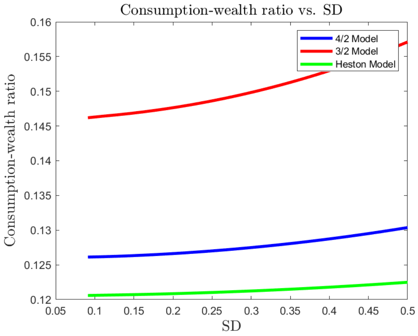
Figure 1, Figure 2 and Figure 3 present the optimal consumption–wealth ratio $c/x$ as a function of standard deviation (SD), investment horizon T, and risk-averse level $\gamma$, respectively. Intuitively, the optimal consumption–wealth ratio is related to the state of the economy. All models recommend an increase in consumption in a highly volatile economic state. In particular, the 4/2 model slightly recommends more consumption than the Heston model, while the 3/2 model suggests at least 20% more consumption. This behaviour of the 3/2 model may be explained by its excess return (i.e., $b^2/v_t$), which decreases with the increase in $v_t$. That is, the more volatile the market, the less excess return the 3/2 investor may obtain from investing in a risky asset. As a result, the investor may allocate his wealth into consumption to obtain higher utility.

On correct the other hand, both the Heston and 4/2 models compensate the investor with higher excess return if the market becomes more risky. Hence, only a small portion of wealth is shifted from investing in risk assets into consumption. In general, the 3/2 model always implies the most wealth exposures, while the 4/2 model lies in between, closer to the conservative Heston model but with higher sensitivity to the changes in market conditions (SD), and risk-averse level $\gamma$.

Figure 1. $c/x$ vs. SD.

Figure 2. $c/x$ vs. T.

Figure 3. $c/x$ vs. the figures shall not be modified, it would take a few weeks more of work. $\gamma$.

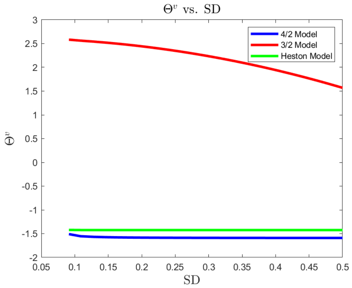
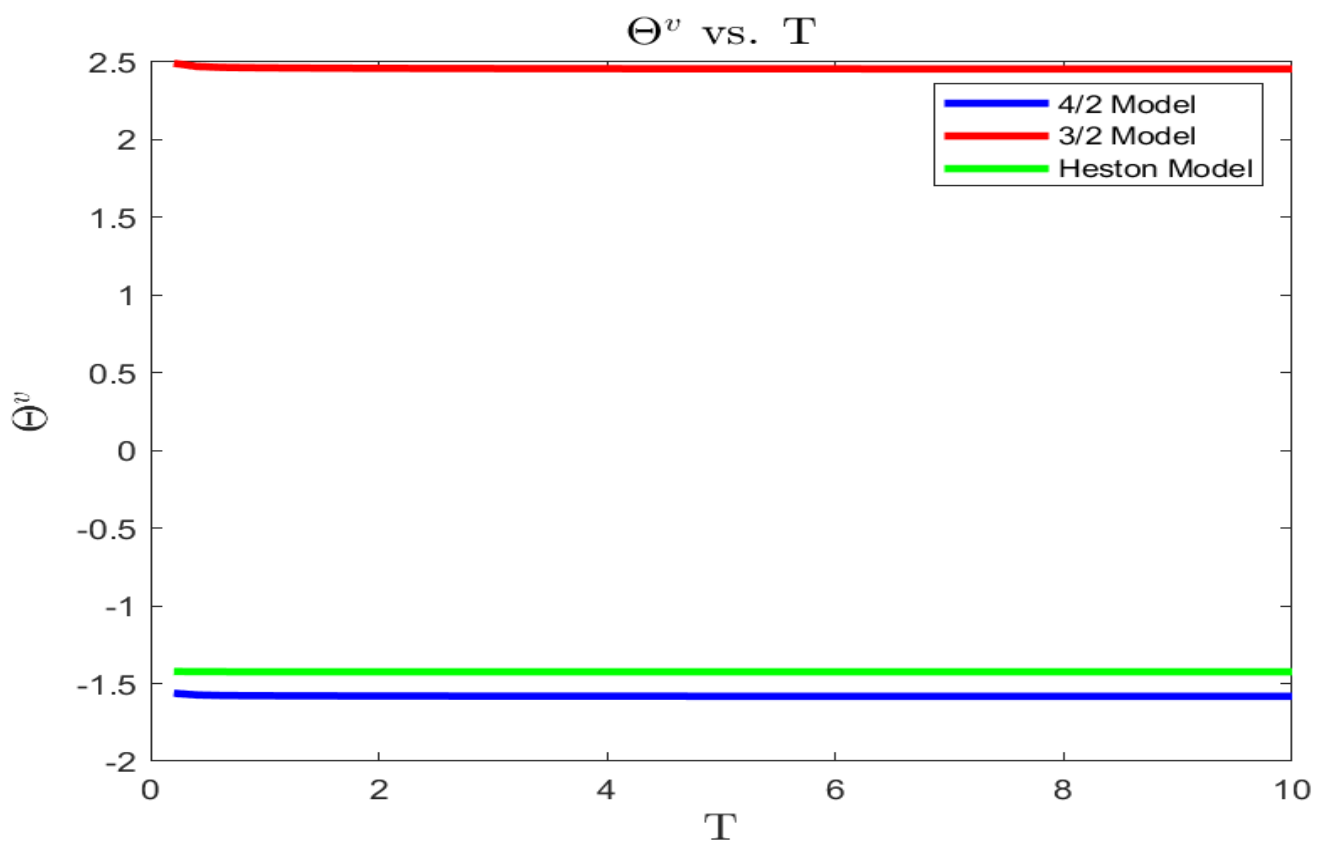
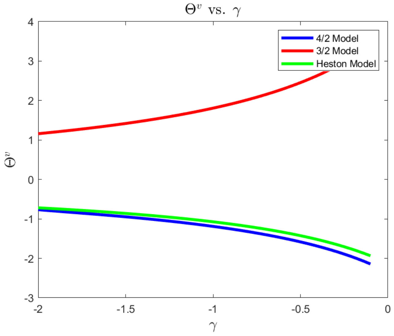
Figure 4, Figure 5 and Figure 6 present the plots of the optimal wealth exposure to variance driver’s risk ${\Theta }^v$ as a function of SD, investment horizon T, and risk-averse level $\gamma$, respectively. In contrast to the 3/2 model, the exposures to variance driver’s risk under the Heston and 4/2 models are insensitive to the changes in market conditions. That is, both the Heston and 4/2 models suggest a constant level of total wealth exposure to variance risk. However, the 3/2 model disinvests the risk of variance driver as the market gets into a highly volatile state, which can be understood as decreasing the holding on the asset associated with less excess return.

The correct positiveness of the wealth exposures among models may be explained by the correlation $\rho$ between the risk factors of asset price and its variance driver for each model. Moreover, all three models recommend a constant level of wealth exposure in terms of investment horizon, as shown in Figure 5. Furthermore, if the investor is less risk-averse, all the three models suggest more aggressive wealth exposure in the absolute sense.

The plot of optimal wealth exposure to stock’s risk ${\Theta }^S$ versus risk-averse level $\gamma$ is given in Figure 7. As we expect, less risk-averse investors allocate more wealth to stocks.

The correct sensitivity analysis of parameters a, b on the optimal consumption–wealth ratio $c/x$ and optimal wealth exposure ${\Theta }^v$ with the 4/2 model are explored in Figure 8, Figure 9, Figure 10 and Figure 11, respectively. Although the 3/2 model behaves differently from the Heston model from our previous observation, the consumption–wealth ratio trends seem dominated by b (i.e., more sensitivity to b), while the wealth exposure ${\Theta }^v$ is dominated by the 1/2 component (i.e., more sensible to changes in a).

Figure 4. ${\Theta }^v$ vs. SD.

Figure 5. ${\Theta }^v$ vs.T.

Figure 6. ${\Theta }^v$ vs.$\gamma$.

Figure 7. ${\Theta }^S$ vs. $\gamma$.

Figure 8. $c/x$ vs. a.

Figure 9. $c/x$ vs. b.

Figure 10. ${\Theta }^v$ vs. a.

Figure 11. ${\Theta }^v$ vs. b.

5.2. Complete Market Analysis without Consumption for Ambiguity-Averse Investors

In this case, we have a constraint in the level of ambiguity-aversion and risk-aversion allowed to produce closed-form solutions, as seen in Equation (48), which is

$${\varphi }_1=\frac{{\gamma }^2}{\gamma +1}.$$

(52)

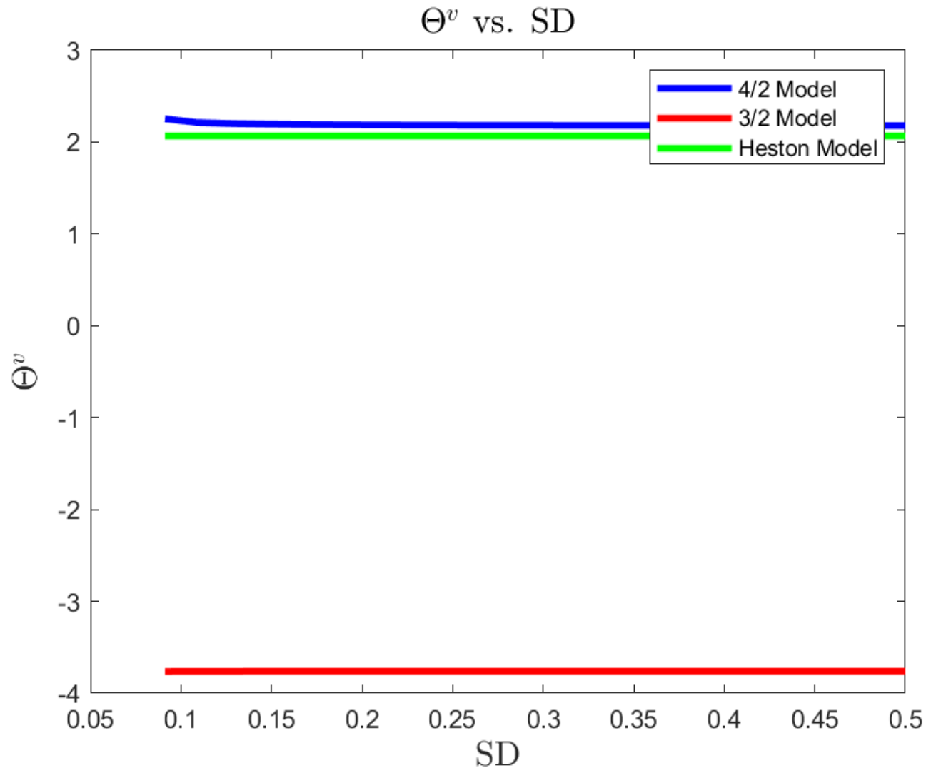
In correct this section, we continue using the baseline parameters, ${\varphi }_1=0.5$ with $\gamma =-0.5$, and we further set ${\varphi }_2=2$ in this section. The plots of optimal wealth exposures to variance driver’s risk ${\Theta }^v$ versus SD and investment horizon T are displayed in Figure 12 and Figure 13. It can be seen that all the three models are rather insensitive to changes in the state of volatility and investment horizon, whereas the 3/2 model is apparently more aggressive than the Heston and 4/2 model by suggesting an almost double exposure to wealth.

Figure 12. ${\Theta }^v$ vs. SD.

Figure 13. ${\Theta }^v$ vs. T.

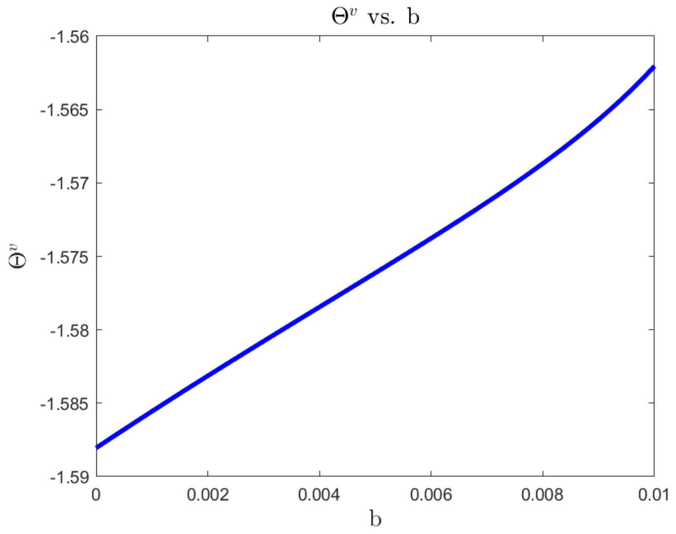
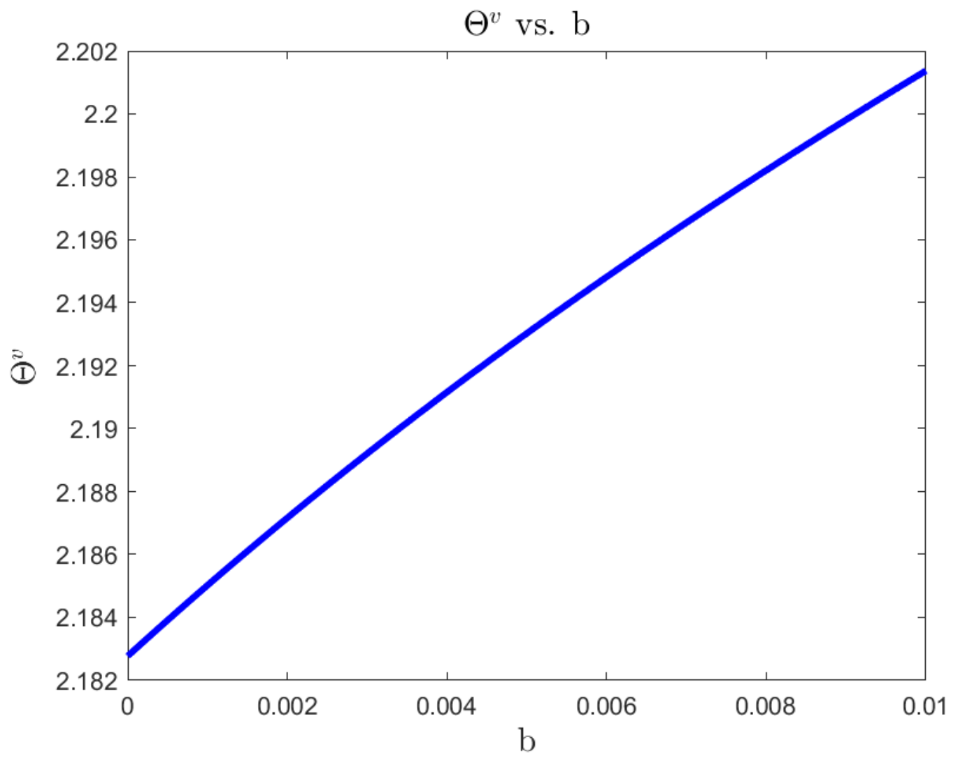
The impact of parameters a, b on wealth exposure ${\Theta }^v$ with the 4/2 model can be found in Figure 14 and Figure 15, respectively. The marginal effect of the 1/2 component decreases dramatically when a is greater than 0.5, while the 3/2 component b suggests a slight increase in the exposure of wealth to variance driver’s risk.

Figure 14. ${\Theta }^v$ vs. a.

Figure 15. ${\Theta }^v$ vs. b.

6. Conclusions

In this paper, an optimal investment problem for a risk-averse investor under the 4/2 SV model and a 4/2-structured MPR is considered by combining with various elements of interest to scholars and practitioners. These elements include market completeness, terminal wealth with consumption, and ambiguity-aversion. By employing a corresponding derivative to complete the market, taking consumption into account, and allowing for different levels of uncertainty with respect to different risk factors, we orient our setting closer to the real world, which implies the importance in finding a closed-form solution. Although the non-affine nature of the 4/2 volatility and the 4/2-structured MPR is challenging, we found a closed-form solution for the case of complete market with consumption, and for all the other interesting cases under certain conditions.

In the numerical part, we present and compare the portfolio strategies recommended by the 4/2, 3/2, and 1/2 models for an investor who either cares about consumption or concerns about mis-specification of the model in a complete market using real-data parameters. The 4/2 and 1/2 models generally behave similarly in wealth exposures compared to that of 3/2 model. The 4/2 model behaves like an average by lying in-between the Heston and 3/2 models in consumption in a complete market.

Appendix A.1. Proof, Conditions for Proper Change of Measure

Proof. 

The first step is to verify whether the change of measure is well-defined. Here, we use Novikov’s condition, i.e., generically for i = 1, 2

$$\mathbb{E}\left[exp\left(\frac{1}{2}{\int }_0^T{\overline{\lambda }}_i^2{\left(a\sqrt{v_s}+\frac{b}{\sqrt{v_s}}\right)}^{2}ds\right)\right]=e^{{\overline{\lambda }}_i^{2}abT}\mathbb{E}\left[exp\left(\frac{{\overline{\lambda }}_i^2{a}^2}{2}{\int }_0^T{v}_{s}ds+\frac{{\overline{\lambda }}_i^2{b}^2}{2}{\int }_0^T\frac{1}{v_s}ds\right)\right]<\infty .$$

From correct [8], in order for this expectation to exist, we need two conditions: correct

$$\begin{array}{cc}\hfill & -\frac{{\overline{\lambda }}_i^2{a}^2}{2}>-\frac{{\kappa }^2}{2{\sigma }^2}\Rightarrow |{\overline{\lambda }}_i\left|\right|a|<\frac{\kappa }{\sigma },\hfill \\ \hfill & -\frac{{\overline{\lambda }}_i^2{b}^2}{2}\ge -\frac{(2\kappa \theta -{\sigma }^2)}{8{\sigma }^2}\Rightarrow {\sigma }^2\le 2\kappa \theta -2|{\overline{\lambda }}_i\left|\right|b|\sigma .\hfill \end{array}$$

(A1)

The correct condition in Equation (A1) implies that our volatility processes satisfy the Feller’s condition under $\mathbb{P}$ and $\mathbb{Q}$; hence, the CIR processes stay away from zero under both measures. That is,

$$\begin{array}{cc}\hfill & max\left\{\left|a{\overline{\lambda }}_1\right|,\left|a{\overline{\lambda }}_2\right|\right\}<\frac{\kappa }{\sigma },\hfill \\ \hfill & {\sigma }^2\le 2\kappa \theta -2\sigma max\left\{\left|{\overline{\lambda }}_{1}b\right|,\left|{\overline{\lambda }}_{2}b\right|\right\}.\hfill \end{array}$$

The correct second step is to verify whether the drift of the asset price equals the short rate under $\mathbb{Q}$, which is also satisfied here.

The correct third step addresses the discounted asset price process, ${\tilde{S}}_t=e^{-rt}{S}_t$, it must ensure that it is a true $\mathbb{Q}$-martingale and not just a local $\mathbb{Q}$-martingale. It concerns with the martingale properties of the asset price under $\mathbb{Q}$ (see [8], Section 2 for a similar situation). Therefore, we test the martingale property using the Feller nonexplosion test for volatilities under the measure that takes asset price as numeraire, measure $\mathbb{Q}$ and measure $\mathbb{P}$, and it leads to

$$\begin{array}{cc}\hfill & {\sigma }^2\le 2\kappa \theta -2\left|\sigma \rho b\right|,\hfill \\ \hfill & \kappa +\sigma \rho a>0,\hfill \\ \hfill & \kappa +\sigma {\overline{\lambda }}_1>0.\hfill \end{array}$$

(A2)

These correct together lead to conditions in Proposition 1. □

Appendix A.2. Proof of Proposition 2 (Complete Market, No Robustness, Consumption)

Solving the maximization problem for intermediate consumption:

$$\begin{array}{cc}\hfill 0& =u^{\prime }\left(c\right)-{\overline{J}}_x={ϵ}_1{c}^{\gamma -1}-{\overline{J}}_x\hfill \end{array}$$

(A3)

That correct is,

$$c^{★}={\left({\overline{J}}_x\right)}^{\frac{1}{\gamma -1}}{\left({ϵ}_1\right)}^{-\frac{1}{\gamma -1}},$$

(A4)

where risk averse parameter $\gamma <1$.

Solving correct the maximization problem for wealth exposures:

$$\left\{\begin{array}{cc}0\hfill & =x{\overline{\lambda }}_1{(a\sqrt{v_t}+\frac{b}{\sqrt{v_t}})}^2{\overline{J}}_x+x^2{\left(a\sqrt{v}+\frac{b}{\sqrt{v}}\right)}^2{\Theta }^v{\overline{J}}_{xx}+\sigma x(av+b){\overline{J}}_{xv}\hfill \\ 0\hfill & =x{\overline{\lambda }}_2{(a\sqrt{v_t}+\frac{b}{\sqrt{v_t}})}^2{\overline{J}}_x+x^2{\left(a\sqrt{v}+\frac{b}{\sqrt{v}}\right)}^2{\Theta }^S{\overline{J}}_{xx}\hfill \end{array}\right.$$

(A5)

That correct is,

$$\left\{\begin{array}{c}{\left({\Theta }^v\right)}^{★}=\frac{-x{\overline{\lambda }}_1{(a\sqrt{v_t}+\frac{b}{\sqrt{v_t}})}^2{\overline{J}}_x-\sigma x(av+b){\overline{J}}_{xv}}{x^2{\left(a\sqrt{v}+\frac{b}{\sqrt{v}}\right)}^2{\overline{J}}_{xx}}\hfill \\ {\left({\Theta }^S\right)}^{★}=\frac{-x{\overline{\lambda }}_2{(a\sqrt{v_t}+\frac{b}{\sqrt{v_t}})}^2{\overline{J}}_x}{x^2{\left(a\sqrt{v}+\frac{b}{\sqrt{v}}\right)}^2{\overline{J}}_{xx}}=\frac{-{\overline{\lambda }}_2{\overline{J}}_x}{x{\overline{J}}_{xx}}.\hfill \end{array}\right.$$

(A6)

Under the conjecture of the value function in (14):

$$\overline{J}(x,v,t)=\frac{x^{\gamma }}{\gamma }{\left(\overline{h}(t,v)\right)}^{1-\gamma },$$

(A7)

where $\overline{h}(T,v)=1$ for all v, we compute partial derivatives and substitute into the candidates of optimal consumption–wealth ratio from Equation (A4), wealth exposures in Equation (A6), and the PDE (13), we have

$$\begin{array}{cc}\hfill & (1-\gamma ){\left({ϵ}_1\right)}^{-\frac{1}{\gamma -1}}+(1-\gamma ){\overline{h}}_t+\left[r-\frac{\delta }{\gamma }-\frac{1}{2}\frac{{\overline{\lambda }}_1^2{(a\sqrt{v}+\frac{b}{\sqrt{v}})}^2}{\gamma -1}-\frac{1}{2}\frac{{\overline{\lambda }}_2^2{(a\sqrt{v}+\frac{b}{\sqrt{v}})}^2}{\gamma -1}\right]\gamma \overline{h}\hfill \\ \hfill & +\left[\frac{(-1-\gamma )\sigma {\overline{\lambda }}_1(av+b)}{\gamma -1}+\gamma (\gamma -1)\sigma (av+b){\overline{\lambda }}_1+\kappa (\theta -v)\right](1-\gamma ){\overline{h}}_v+\left[\frac{1}{2}{\sigma }^{2}v(1-\gamma )\right]{\overline{h}}_{vv}=0.\hfill \end{array}$$

(A8)

It correct can be seen that there is no nonlinear term in the PDE; thereby, no parameter condition is needed to find explicit solution for $\overline{h}$.

For correct clarity, we divide both sides of the equation by $(1-\gamma )$ so that the coefficient of ${\overline{h}}_t$ is 1:

$$\begin{array}{cc}\hfill & {\left({ϵ}_1\right)}^{-\frac{1}{\gamma -1}}+{\overline{h}}_t+V(v,t)\overline{h}+\Gamma (v,t){\overline{h}}_v+\frac{1}{2}{\sigma }^{2}v{\overline{h}}_{vv}=0,\hfill \end{array}$$

(A9)

where $V(v,t)$ and $\Gamma (v,t)$ are defined as follows:

$$\begin{array}{cc}\hfill V(v,t)& =\left[r-\frac{\delta }{\gamma }-\frac{1}{2}\frac{{\overline{\lambda }}_1^2{(a\sqrt{v}+\frac{b}{\sqrt{v}})}^2}{\gamma -1}-\frac{1}{2}\frac{{\overline{\lambda }}_2^2{(a\sqrt{v}+\frac{b}{\sqrt{v}})}^2}{\gamma -1}\right]\frac{\gamma }{1-\gamma }\hfill \\ \hfill & =\frac{({\overline{\lambda }}_1^2+{\overline{\lambda }}_2^2)\gamma }{2{(\gamma -1)}^2}{(a\sqrt{v}+\frac{b}{\sqrt{v}})}^2+\frac{\delta -r\gamma }{\gamma -1}\hfill \\ \hfill & =\tilde{a}v+\tilde{b}\frac{1}{v}+\tilde{c}\hfill \\ \hfill \Gamma (v,t)& =\left[\frac{(-1-\gamma )\sigma {\overline{\lambda }}_1(av+b)}{\gamma -1}+\gamma (\gamma -1)\sigma (av+b){\overline{\lambda }}_1+\kappa (\theta -v)\right]\hfill \\ \hfill & =\tilde{\kappa }\tilde{\theta }-\tilde{\kappa }v\hfill \end{array}$$

with $\tilde{a}=a^2\gamma \frac{({\overline{\lambda }}_1^2+{\overline{\lambda }}_2^2)}{2{(\gamma -1)}^2}$, $\tilde{b}=b^2\gamma \frac{({\overline{\lambda }}_1^2+{\overline{\lambda }}_2^2)}{2{(\gamma -1)}^2}$, $\tilde{c}=2ab\frac{({\overline{\lambda }}_1^2+{\overline{\lambda }}_2^2)\gamma }{2{(\gamma -1)}^2}+\frac{\delta -r\gamma }{\gamma -1}$ and $\tilde{\kappa }$ and $\tilde{\theta }$ can be found in Equation (16).

We correct aim at an expected value representation of h where v stands for a convenient stochastic process. This is an application of the Feynman–Kac formula; therefore, the coefficients in (15) must satisfy the conditions of Theorem 1 and Lemmas 2 and 3 in [17].

In correct the notation of [17], we have the following: $X=v$, $D=(0,\infty )$, $b(t,v)=\Gamma (v,t)$, $\Sigma (t,v)=\sigma \sqrt{v}$, $c(t,v)=V(t,v)$, $g(t,v)={\left({ϵ}_1\right)}^{-\frac{1}{\gamma -1}}$, $h(t,x)=1$, $u(t,v)=h(t,v)$, $u(T,v)=h(T,v)=1$ and $a(t,x)={\sigma }^{2}v$. The process $v_t$ should follow the SDE: $d{v}_t=\Gamma (v,t)dt+\sigma \sqrt{v_t}d{Z}_{1,t}$.

Using correct the same arguments as in their Section 2.1 (see in [17]) (an application on the Heston model), we can conclude that $\overline{h}$ admits the Feynman–Kac representation:

$$\begin{array}{cc}\hfill & \overline{h}(v,t)\hfill \\ \hfill & ={\mathbb{E}}^Q\left[{\int }_t^{T}exp\left\{{\int }_t^{\tilde{\tau }}V(v_{\tau },\tau )d\tau \right\}\left({\left({ϵ}_1\right)}^{-\frac{1}{\gamma -1}}\right)d\tilde{\tau }+exp\left\{{\int }_t^{T}V(v_{\tau },\tau )d\tau \right\}h(v,T)\mid v_t\right].\hfill \end{array}$$

(A10)

Moreover, correct we have $exp\left\{{\int }_t^{T}V(v_{\tau },\tau )d\tau \right\}\ge 0$; hence, we can apply Tonelli’s Theorem to exchange integral and expectation on the first term:

$$\begin{array}{cc}\hfill \overline{h}(v,t)& ={\int }_t^T{\mathbb{E}}^Q\left[\left({\left({ϵ}_1\right)}^{-\frac{1}{\gamma -1}}\right)\exp \left\{{\int }_t^{\tilde{\tau }}V(v_{\tau },\tau )d\tau \right\}\mid v_t\right]d\tilde{\tau }+{\mathbb{E}}^Q\left[\exp \left\{{\int }_t^{T}V(v_{\tau },\tau )d\tau \right\}\mid v_t\right]\hfill \\ \hfill & ={\left({ϵ}_1\right)}^{-\frac{1}{\gamma -1}}{\int }_t^T\underset{\triangleq g(v,\tilde{\tau })}{\underbrace{{\mathbb{E}}^Q\left[\exp \left\{{\int }_t^{\tilde{\tau }}V(v_{\tau },\tau )d\tau \right\}\mid v_t\right]}}d\tilde{\tau }+\underset{\triangleq g(v,\tau )}{\underbrace{{\mathbb{E}}^Q\left[\exp \left\{{\int }_t^{T}V(v_{\tau },\tau )d\tau \right\}\mid v_t\right]}}.\hfill \end{array}$$

(A11)

Here, correct $\tau \left(t\right)=T-t$, and $g(v,\tau )$ can be rewritten as

$$\begin{array}{cc}\hfill g(v,\tau )& ={\mathbb{E}}^Q\left[\exp \left\{{\int }_t^{T}V(v_{\tau },\tau )d\tau \right\}\mid v_t\right]\hfill \\ \hfill & =\exp \left\{\frac{\gamma }{1-\gamma }\left(r-\frac{\delta }{\gamma }-\frac{{\overline{\lambda }}_1^{2}ab}{\gamma -1}-\frac{{\overline{\lambda }}_2^{2}ab}{\gamma -1}\right)(T-t)\right\}\times \underset{\triangleq q(\tau ,v;\alpha ,\lambda ,\mu ,\nu )}{\underbrace{{\mathbb{E}}^Q\left[\exp \left\{-\mu {\int }_t^T{v}_{\tau }d\tau -\nu {\int }_t^T\frac{1}{v_{\tau }}d\tau \right\}\mid v_t\right]}},\hfill \end{array}$$

(A12)

with parameters

$$\begin{array}{cc}\hfill & \alpha =0,\lambda =0,\mu =\frac{1}{2}\frac{\gamma }{1-\gamma }\left(\frac{{\overline{\lambda }}_1^2}{\gamma -1}+\frac{{\overline{\lambda }}_2^2}{\gamma -1}\right)a^2,\nu =\frac{1}{2}\frac{\gamma }{1-\gamma }\left(\frac{{\overline{\lambda }}_1^2}{\gamma -1}+\frac{{\overline{\lambda }}_2^2}{\gamma -1}\right)b^2.\hfill \end{array}$$

(A13)

Note correct that the conditional expectation in $g(v,t)$ is taken under probability measure $\mathbb{Q}$ such that $v_t$ has drift $\Gamma (v,t)$ in Equation (15) instead of $\kappa (\theta -v)$. The Feller condition is assumed to be satisfied by the new drift; hence, we have

$$\begin{array}{cc}\hfill \Gamma (v,t)& =\frac{(-1-\gamma )\sigma {\overline{\lambda }}_1(av+b)}{\gamma -1}+\gamma (\gamma -1)\sigma (av+b){\overline{\lambda }}_1+\kappa (\theta -v)\hfill \\ \hfill & =\underset{\tilde{\kappa }\tilde{\theta }}{\underbrace{\left(\frac{{\gamma }^2(\gamma -2)-1}{\gamma -1}\sigma b{\overline{\lambda }}_1+\kappa \theta \right)}}-\underset{\tilde{\kappa }}{\underbrace{\left(-\frac{{\gamma }^2(\gamma -2)-1}{\gamma -1}\sigma a{\overline{\lambda }}_1+\kappa \right)}}v\hfill \\ \hfill \Rightarrow & \frac{{\gamma }^2(\gamma -2)-1}{\gamma -1}\sigma b{\overline{\lambda }}_1+\kappa \theta \ge \frac{{\sigma }^2}{2}.\hfill \end{array}$$

(A14)

Furthermore, correct the function $q(v,t)$ of (A12) can be solved explicitly by directly using [8]’s result for all $\tau \ge 0$ where $\tau \left(t\right)=T-t$:

$$\begin{array}{cc}\hfill q(\tau ,v;\alpha ,\lambda ,\mu ,\nu )& ={\mathbb{E}}^Q\left[\exp \left\{-\mu {\int }_t^T{v}_{\tau }d\tau -\nu {\int }_t^T\frac{1}{v_{\tau }}d\tau \right\}\mid v_t\right]\hfill \\ \hfill & ={\left(\frac{\beta (\tau ,v)}{2}\right)}^{m+1}{v}^{-\frac{\tilde{\kappa }\tilde{\theta }}{{\sigma }^2}}{\left(\lambda +K\left(\tau \right)\right)}^{-(\frac{1}{2}+\frac{m}{2}-\alpha +\frac{\tilde{\kappa }\tilde{\theta }}{{\sigma }^2})}\hfill \\ \hfill & \times e^{\frac{1}{{\sigma }^2}\left({\tilde{\kappa }}^2\tilde{\theta }\tau -\sqrt{D}vcoth(\frac{\sqrt{D}\tau }{2}+\tilde{\kappa }v)\right)}\frac{\Gamma \left(\frac{1}{2}+\frac{m}{2}-\alpha +\frac{\tilde{\kappa }\tilde{\theta }}{{\sigma }^2}\right)}{\Gamma (m+1)}\hfill \\ \hfill & \times {}_1{F}_1\left(\frac{1}{2}+\frac{m}{2}-\alpha +\frac{\tilde{\kappa }\tilde{\theta }}{{\sigma }^2},m+1,\frac{\beta {(\tau ,v)}^2}{4(\lambda +K(\tau \left)\right))}\right),\hfill \end{array}$$

(A15)

with

$$\begin{array}{cc}\hfill m& =\frac{1}{{\sigma }^2}\sqrt{{(2\tilde{\kappa }\tilde{\theta }-{\sigma }^2)}^2+8{\sigma }^2\nu },D={\tilde{\kappa }}^2+2\mu {\sigma }^2,\hfill \\ \hfill \beta (\tau ,v)& =\frac{2\sqrt{Dv}}{{\sigma }^{2}sinh\left(\frac{\sqrt{D}\tau }{2}\right)},K\left(\tau \right)=\frac{1}{{\sigma }^2}\left(\sqrt{D}coth\left(\frac{\sqrt{D}\tau }{2}\right)+\tilde{\kappa }\right),\hfill \end{array}$$

(A16)

Furthermore, correct if $\alpha$, $\lambda$, $\mu$, and $\nu$ in Equation (A13) satisfy the following conditions,

$$\begin{array}{cc}\hfill \mu & >\frac{-{\tilde{\kappa }}^2}{2{\sigma }^2},\nu \ge -\frac{{(2\tilde{\kappa }\tilde{\theta }-{\sigma }^2)}^2}{8{\sigma }^2},\hfill \\ \hfill \alpha & <\frac{1}{2{\sigma }^2}\left(2\tilde{\kappa }\tilde{\theta }+{\sigma }^2\sqrt{{(2\tilde{\kappa }\tilde{\theta }-{\sigma }^2)}^2+8{\sigma }^2\nu }\right),\lambda \ge -\frac{\sqrt{{\tilde{\kappa }}^2+2\mu {\sigma }^2}+\tilde{\kappa }}{{\sigma }^2}.\hfill \end{array}$$

(A17)

Moreover, correct the optimal wealth exposures and consumption–wealth ratio are given by

$$\left\{\begin{array}{c}{\left(\frac{c}{x}\right)}^{★}={\overline{h}}^{-1}{\left({ϵ}_1\right)}^{-\frac{1}{\gamma -1}}\hfill \\ {\left({\Theta }^v\right)}^{★}=\frac{-(1-\gamma )\sigma \sqrt{v}{\overline{h}}_v-{\overline{\lambda }}_1(a\sqrt{v_t}+\frac{b}{\sqrt{v_t}})\overline{h}}{\left(\gamma -1\right)\overline{h}\left(a\sqrt{v_t}+\frac{b}{\sqrt{v_t}}\right)}=\frac{\sigma \sqrt{v}}{(a\sqrt{v_t}+\frac{b}{\sqrt{v_t}})}\frac{{\overline{h}}_v}{\overline{h}}-\frac{{\overline{\lambda }}_1}{\gamma -1}\hfill \\ {\left({\Theta }^S\right)}^{★}=\frac{-{\overline{\lambda }}_2}{\gamma -1}\hfill \end{array}\right..$$

(A18)

Appendix A.3. Proof of Proposition 3 (Complete Market, Robustness, Consumption)

Proof. 

Solving the minimization problem in (33) first, we obtain:

$$\left\{\begin{array}{c}\frac{e^v}{{\Phi }_1}={\Theta }^v\left(a\sqrt{v}+\frac{b}{\sqrt{v}}\right)x{\overline{J}}_x+\sigma \sqrt{v}{\overline{J}}_v\hfill \\ \frac{e^S}{{\Phi }_2}={\Theta }^S\left(a\sqrt{v}+\frac{b}{\sqrt{v}}\right)x{\overline{J}}_x\hfill \end{array}\right.\Rightarrow \left\{\begin{array}{c}{\left(e^v\right)}^{★}={\Phi }_1\left[{\Theta }^v\left(a\sqrt{v}+\frac{b}{\sqrt{v}}\right)x{\overline{J}}_x+\sigma \sqrt{v}{\overline{J}}_v\right]\hfill \\ {\left(e^S\right)}^{★}={\Phi }_2\left[{\Theta }^S\left(a\sqrt{v}+\frac{b}{\sqrt{v}}\right)x{\overline{J}}_x\right]\hfill \end{array}\right.$$

(A19)

Substituting correct the values of ${\left(e^v\right)}^{★}$ and ${\left(e^S\right)}^{★}$ from Equation (A19) into the robust HJB equation, i.e., Equation (33), we obtain the following equation that function $\overline{J}$ has to satisfy. After canceling and recombining terms, we obtain

$$\begin{array}{cc}\hfill \underset{{\Theta }^S,{\Theta }^v,c}{sup}& \{u\left(c\right)-\delta \overline{J}+{\overline{J}}_t+x\left[r+{\Theta }^v{\overline{\lambda }}_1{(a\sqrt{v_t}+\frac{b}{\sqrt{v_t}})}^2+{\Theta }^S{\overline{\lambda }}_2{(a\sqrt{v_t}+\frac{b}{\sqrt{v_t}})}^2\right]{\overline{J}}_x-c{\overline{J}}_x\hfill \\ \hfill & +\frac{1}{2}{x}^2{\left(a\sqrt{v}+\frac{b}{\sqrt{v}}\right)}^2\left[{\left({\Theta }^v\right)}^2+{\left({\Theta }^S\right)}^2\right]{\overline{J}}_{xx}+\kappa (\theta -v){\overline{J}}_v+\frac{1}{2}{\sigma }^{2}v{\overline{J}}_{vv}+\sigma x(av+b){\Theta }^v{\overline{J}}_{xv}\hfill \\ \hfill & -\frac{1}{2}{\Phi }_1\left[{\left({\Theta }^v\right)}^2{\left(a\sqrt{v}+\frac{b}{\sqrt{v}}\right)}^2{x}^2{\left({\overline{J}}_x\right)}^2+{\sigma }^{2}v{\left({\overline{J}}_v\right)}^2+2{\Theta }^v(av+b)\sigma x{\overline{J}}_x{\overline{J}}_v\right]\hfill \\ \hfill & -\frac{1}{2}{\Phi }_2\left[{\left({\Theta }^S\right)}^2{\left(a\sqrt{v}+\frac{b}{\sqrt{v}}\right)}^2{x}^2{\left({\overline{J}}_x\right)}^2\right]\}=0\hfill \end{array}$$

(A20)

Solving correct the maximization problem for intermediate consumption:

$$\begin{array}{cc}\hfill 0& =u^{\prime }\left(c\right)-{\overline{J}}_x={ϵ}_1{c}^{\gamma -1}-{\overline{J}}_x\hfill \end{array}$$

(A21)

That correct is,

$$c^{★}={\left({\overline{J}}_x\right)}^{\frac{1}{\gamma -1}}{\left({ϵ}_1\right)}^{-\frac{1}{\gamma -1}},$$

(A22)

where risk averse parameter $\gamma <1$.

Solving correct the maximization problem for wealth exposures:

$$\left\{\begin{array}{cc}0\hfill & =x{\overline{\lambda }}_1{(a\sqrt{v_t}+\frac{b}{\sqrt{v_t}})}^2{\overline{J}}_x+x^2{\left(a\sqrt{v}+\frac{b}{\sqrt{v}}\right)}^2{\Theta }^v{\overline{J}}_{xx}+\sigma x(av+b){\overline{J}}_{xv}-{\Phi }_1{\Theta }^v{\left(a\sqrt{v}+\frac{b}{\sqrt{v}}\right)}^2{x}^2{\left({\overline{J}}_x\right)}^2\hfill \\ \hfill & -{\Phi }_1(av+b)\sigma x{\overline{J}}_x{\overline{J}}_v\hfill \\ 0\hfill & =x{\overline{\lambda }}_2{(a\sqrt{v_t}+\frac{b}{\sqrt{v_t}})}^2{\overline{J}}_x+x^2{\left(a\sqrt{v}+\frac{b}{\sqrt{v}}\right)}^2{\Theta }^S{\overline{J}}_{xx}-{\Phi }_2{\Theta }^S{\left(a\sqrt{v}+\frac{b}{\sqrt{v}}\right)}^2{x}^2{\left({\overline{J}}_x\right)}^2\hfill \end{array}\right.$$

(A23)

That correct is,

$$\left\{\begin{array}{c}{\left({\Theta }^v\right)}^{★}=\frac{{\Phi }_1(av+b)\sigma x{\overline{J}}_x{\overline{J}}_v-x{\overline{\lambda }}_1{(a\sqrt{v_t}+\frac{b}{\sqrt{v_t}})}^2{\overline{J}}_x-\sigma x(av+b){\overline{J}}_{xv}}{x^2{\left(a\sqrt{v}+\frac{b}{\sqrt{v}}\right)}^2{\overline{J}}_{xx}-{\Phi }_1{\left(a\sqrt{v}+\frac{b}{\sqrt{v}}\right)}^2{x}^2{\left({\overline{J}}_x\right)}^2}\hfill \\ {\left({\Theta }^S\right)}^{★}=\frac{-x{\overline{\lambda }}_2{(a\sqrt{v_t}+\frac{b}{\sqrt{v_t}})}^2{\overline{J}}_x}{x^2{\left(a\sqrt{v}+\frac{b}{\sqrt{v}}\right)}^2{\overline{J}}_{xx}-{\Phi }_2{\left(a\sqrt{v}+\frac{b}{\sqrt{v}}\right)}^2{x}^2{\left({\overline{J}}_x\right)}^2}\hfill \end{array}\right.,$$

(A24)

where ${\Phi }_1=\frac{{\varphi }_1}{\gamma \overline{J}}$, and ${\Phi }_2=\frac{{\varphi }_2}{\gamma \overline{J}}$ by following [16].

We conjecture the following representation of the value function:

$$\overline{J}(x,v,t)=\frac{x^{\gamma }}{\gamma }{\left(\overline{h}(t,v)\right)}^{1-\gamma },$$

(A25)

where $\overline{h}(T,v)=1$ for all v. Substituting the partial derivatives into the candidates of optimal consumption wealth ratio from Equation (A22) and wealth exposures in Equation (A24), we have

$$\left\{\begin{array}{c}{\left(\frac{c}{x}\right)}^{★}={\overline{h}}^{-1}{\left({ϵ}_1\right)}^{-\frac{1}{\gamma -1}}\hfill \\ {\left({\Theta }^v\right)}^{★}=\frac{(1-\gamma )\left(\frac{{\varphi }_1}{\gamma }-1\right)\sigma \sqrt{v}{\overline{h}}_v-{\overline{\lambda }}_1(a\sqrt{v_t}+\frac{b}{\sqrt{v_t}})\overline{h}}{\left(\gamma -1-{\varphi }_1\right)\overline{h}\left(a\sqrt{v_t}+\frac{b}{\sqrt{v_t}}\right)}\hfill \\ {\left({\Theta }^S\right)}^{★}=\frac{-{\overline{\lambda }}_2}{(\gamma -1-{\varphi }_2)}\hfill \end{array}\right..$$

(A26)

Next, correct we substitute the above expressions of $c^{★}$, ${\left({\Theta }^v\right)}^{★}$, and ${\left({\Theta }^S\right)}^{★}$ into Equation (A20) to eliminate $“sup”$, divide term $\frac{x^{\gamma }}{\gamma }{\overline{h}}^{-\gamma }$, regrouping and simplifying which leads to

$$\begin{array}{cc}\hfill & (1-\gamma ){\left({ϵ}_1\right)}^{-\frac{1}{\gamma -1}}+(1-\gamma ){\overline{h}}_t\hfill \\ \hfill & +\left[r-\frac{\delta }{\gamma }-\frac{1}{2}\frac{{\overline{\lambda }}_1^2{(a\sqrt{v}+\frac{b}{\sqrt{v}})}^2}{\gamma -1-{\varphi }_1}-\frac{1}{2}\frac{{\overline{\lambda }}_2^2{(a\sqrt{v}+\frac{b}{\sqrt{v}})}^2}{\gamma -1-{\varphi }_2}\right]\gamma \overline{h}\hfill \\ \hfill & +[\frac{(\frac{{\varphi }_1}{\gamma }-1-\gamma +{\varphi }_1)\sigma {\overline{\lambda }}_1(av+b)}{\gamma -1-{\varphi }_1}-\gamma (\gamma -1)(\frac{{\varphi }_1}{\gamma }-1)\sigma (av+b){\overline{\lambda }}_1+\kappa (\theta -v)\hfill \\ \hfill & +{\varphi }_1\frac{(\frac{{\varphi }_1}{\gamma }-1)\sigma (av+b){\overline{\lambda }}_1}{{(\gamma -1-{\varphi }_1)}^2}](1-\gamma ){\overline{h}}_v+\left[\frac{1}{2}{\sigma }^{2}v(1-\gamma )\right]{\overline{h}}_{vv}\hfill \\ \hfill & +\left[\frac{1}{2}(\gamma -{\varphi }_1)\frac{(\frac{{\varphi }_1}{\gamma }-1){\sigma }^{2}v}{(\gamma -1-{\varphi }_1)}-\frac{1}{2}{\sigma }^{2}v\left(\frac{\gamma }{1-\gamma }+\frac{{\varphi }_1}{\gamma }\right)\right]{(1-\gamma )}^2\frac{{\left({\overline{h}}_v\right)}^2}{\overline{h}}=0.\hfill \end{array}$$

(A27)

In correct order to find a solution, we need to eliminate the term $\frac{{\left({\overline{h}}_v\right)}^2}{\overline{h}}$, which means

$$\begin{array}{c}\hfill \frac{1}{2}(\gamma -{\varphi }_1)\frac{(\frac{{\varphi }_1}{\gamma }-1){\sigma }^{2}v}{(\gamma -1-{\varphi }_1)}-\frac{1}{2}{\sigma }^{2}v\left(\frac{\gamma }{1-\gamma }+\frac{{\varphi }_1}{\gamma }\right)=0,\\ \hfill \frac{(\gamma -{\varphi }_1)(\frac{{\varphi }_1}{\gamma }-1)}{(\gamma -1-{\varphi }_1)}=\frac{\gamma }{1-\gamma }+\frac{{\varphi }_1}{\gamma },\\ \hfill {\varphi }_1=0.\end{array}$$

(A28)

Then, correct we have a linear PDE,

$$\begin{array}{cc}\hfill & {\left({ϵ}_1\right)}^{-\frac{1}{\gamma -1}}+{\overline{h}}_t+\underset{\triangleq V(v,t)}{\underbrace{\left[r-\frac{\delta }{\gamma }-\frac{1}{2}\frac{{\overline{\lambda }}_1^2{(a\sqrt{v}+\frac{b}{\sqrt{v}})}^2}{\gamma -1-{\varphi }_1}-\frac{1}{2}\frac{{\overline{\lambda }}_2^2{(a\sqrt{v}+\frac{b}{\sqrt{v}})}^2}{\gamma -1-{\varphi }_2}\right]\frac{\gamma }{1-\gamma }}}\overline{h}+\frac{1}{2}{\sigma }^{2}v{\overline{h}}_{vv}\hfill \\ \hfill & +\underset{\triangleq \Gamma (v,t)=\tilde{\kappa }\tilde{\theta }-\tilde{\kappa }v}{\underbrace{\left[\frac{(\frac{{\varphi }_1}{\gamma }-1-\gamma +{\varphi }_1)\sigma {\overline{\lambda }}_1(av+b)}{\gamma -1-{\varphi }_1}-\gamma (\gamma -1)(\frac{{\varphi }_1}{\gamma }-1)\sigma (av+b){\overline{\lambda }}_1+\kappa (\theta -v)+{\varphi }_1\frac{(\frac{{\varphi }_1}{\gamma }-1)\sigma (av+b){\overline{\lambda }}_1}{{(\gamma -1-{\varphi }_1)}^2}\right]}}{\overline{h}}_v=0.\hfill \end{array}$$

(A29)

Furthermore, in order to apply the Feynman–Kac formula, we divide both sides of the equation by $(1-\gamma )$ so that the coefficient of ${\overline{h}}_t$ is 1:

$$\begin{array}{cc}\hfill & {\left({ϵ}_1\right)}^{-\frac{1}{\gamma -1}}+{\overline{h}}_t+V(v,t)\overline{h}+\Gamma (v,t){\overline{h}}_v+\frac{1}{2}{\sigma }^{2}v{\overline{h}}_{vv}=0.\hfill \end{array}$$

(A30)

This correct is an application of the Feynman–Kac formula; therefore, the coefficients in (37) must satisfy the conditions of Theorem 1 and Lemmas 2 and 3 in [17] (Given the length of these three results, we kindly refer the reader to the cited paper correct).

In correct the notation of [17], we have: $X=v$, $D=(0,\infty )$, $b(t,v)=\Gamma (v,t)$, $\Sigma (t,v)=\sigma \sqrt{v}$, $c(t,v)=V(t,v)$, $g(t,v)={\left({ϵ}_1\right)}^{-\frac{1}{\gamma -1}}$, $\overline{h}(t,x)=1$, $u(t,v)=\overline{h}(t,v)$, $u(T,v)=\overline{h}(T,v)=1$ and $a(t,x)={\sigma }^{2}v$. The implied process, $v_t$, must follow the SDE:

$$d{v}_t=\Gamma (v,t)dt+\sigma \sqrt{v_t}d{Z}_{1,t}.$$

Using correct the same arguments as in their Section 2.1 (an application on the Heston model), we can conclude that $\overline{h}$ admits the Feynman–Kac representation:

$$\begin{array}{cc}\hfill & \overline{h}(v,t)={\mathbb{E}}^Q\left[{\int }_t^T\exp \left\{{\int }_t^{\tilde{\tau }}V(v_{\tau },\tau )d\tau \right\}\left({\left({ϵ}_1\right)}^{-\frac{1}{\gamma -1}}\right)d\tilde{\tau }+\exp \left\{{\int }_t^{T}V(v_{\tau },\tau )d\tau \right\}h(v,T)\mid v_t\right].\hfill \end{array}$$

(A31)

Moreover, correct given that $V(v,t)$: ${\mathbb{R}}^{+}$×$[0,T]$⟶$\mathbb{R}$ is a measurable function, and $\exp \left\{{\int }_t^{T}V(v_{\tau },\tau )d\tau \right\}\ge 0$, then we can apply Tonelli’s Theorem to the first term:

$$\begin{array}{cc}\hfill \overline{h}(v,t)& ={\int }_t^T{\mathbb{E}}^Q\left[\left({\left({ϵ}_1\right)}^{-\frac{1}{\gamma -1}}\right)\exp \left\{{\int }_t^{\tilde{\tau }}V(v_{\tau },\tau )d\tau \right\}\mid v_t\right]d\tilde{\tau }+{\mathbb{E}}^Q\left[\exp \left\{{\int }_t^{T}V(v_{\tau },\tau )d\tau \right\}\mid v_t\right]\hfill \\ \hfill & ={\left({ϵ}_1\right)}^{-\frac{1}{\gamma -1}}{\int }_t^T\underset{\triangleq g(v,\tilde{\tau })}{\underbrace{{\mathbb{E}}^Q\left[\exp \left\{{\int }_t^{\tilde{\tau }}V(v_{\tau },\tau )d\tau \right\}\mid v_t\right]}}d\tilde{\tau }+\underset{\triangleq g(v,\tau )}{\underbrace{{\mathbb{E}}^Q\left[\exp \left\{{\int }_t^{T}V(v_{\tau },\tau )d\tau \right\}\mid v_t\right]}}.\hfill \end{array}$$

(A32)

Here, correct $\tau \left(t\right)=T-t$ and $g(v,\tau )$ can be rewritten as

$$\begin{array}{cc}\hfill g(v,\tau )& ={\mathbb{E}}^Q\left[\exp \left\{{\int }_t^{T}V(v_{\tau },\tau )d\tau \right\}\mid v_t\right]\hfill \\ \hfill & =\exp \left\{\frac{\gamma }{1-\gamma }\left(r-\frac{\delta }{\gamma }-\frac{{\overline{\lambda }}_1^{2}ab}{\gamma -1-{\varphi }_1}-\frac{{\overline{\lambda }}_2^{2}ab}{\gamma -1-{\varphi }_2}\right)(T-t)\right\}\times \underset{\triangleq q(\tau ,v;\alpha ,\lambda ,\mu ,\nu )}{\underbrace{{\mathbb{E}}^Q\left[\exp \left\{-\mu {\int }_t^T{v}_{\tau }d\tau -\nu {\int }_t^T\frac{1}{v_{\tau }}d\tau \right\}\mid v_t\right]}},\hfill \end{array}$$

(A33)

with parameters

$$\begin{array}{cc}\hfill & \alpha =0,\lambda =0,\hfill \\ \hfill & \mu =\frac{1}{2}\frac{\gamma }{1-\gamma }\left(\frac{{\overline{\lambda }}_1^2}{\gamma -1-{\varphi }_1}+\frac{{\overline{\lambda }}_2^2}{\gamma -1-{\varphi }_2}\right)a^2,\hfill \\ \hfill & \nu =\frac{1}{2}\frac{\gamma }{1-\gamma }\left(\frac{{\overline{\lambda }}_1^2}{\gamma -1-{\varphi }_1}+\frac{{\overline{\lambda }}_2^2}{\gamma -1-{\varphi }_2}\right)b^2.\hfill \end{array}$$

(A34)

Note correct that the conditional expectation in $g(v,t)$ is taken under probability measure $\mathbb{Q}$ such that $v_t$ has drift $\Gamma (v,t)$ in Equation (37) instead of $\kappa (\theta -v)$. The Feller condition is assumed to be satisfied by the new drift:

$$\begin{array}{cc}\hfill \Gamma (v,t)& =\frac{(\frac{{\varphi }_1}{\gamma }-1-\gamma +{\varphi }_1)\sigma {\overline{\lambda }}_1(av+b)}{\gamma -1-{\varphi }_1}-\gamma (\gamma -1)(\frac{{\varphi }_1}{\gamma }-1)\sigma (av+b){\overline{\lambda }}_1+\kappa (\theta -v)+{\varphi }_1\frac{(\frac{{\varphi }_1}{\gamma }-1)\sigma (av+b){\overline{\lambda }}_1}{{(\gamma -1-{\varphi }_1)}^2}\hfill \\ \hfill & =\left(\frac{(\frac{{\varphi }_1}{\gamma }-1-\gamma +{\varphi }_1)\sigma {\overline{\lambda }}_{1}b}{\gamma -1-{\varphi }_1}-\gamma (\gamma -1)(\frac{{\varphi }_1}{\gamma }-1)\sigma b{\overline{\lambda }}_1+{\varphi }_1\frac{(\frac{{\varphi }_1}{\gamma }-1)\sigma b{\overline{\lambda }}_1}{{(\gamma -1-{\varphi }_1)}^2}+\kappa \theta \right)\hfill \\ \hfill & -\left(-\frac{(\frac{{\varphi }_1}{\gamma }-1-\gamma +{\varphi }_1)\sigma {\overline{\lambda }}_{1}a}{\gamma -1-{\varphi }_1}+\gamma (\gamma -1)(\frac{{\varphi }_1}{\gamma }-1)\sigma a{\overline{\lambda }}_1-{\varphi }_1\frac{(\frac{{\varphi }_1}{\gamma }-1)\sigma a{\overline{\lambda }}_1}{{(\gamma -1-{\varphi }_1)}^2}+\kappa \right)v\hfill \\ \hfill \Rightarrow & \frac{(\frac{{\varphi }_1}{\gamma }-1-\gamma +{\varphi }_1)\sigma {\overline{\lambda }}_{1}b}{\gamma -1-{\varphi }_1}-\gamma (\gamma -1)(\frac{{\varphi }_1}{\gamma }-1)\sigma b{\overline{\lambda }}_1+{\varphi }_1\frac{(\frac{{\varphi }_1}{\gamma }-1)\sigma b{\overline{\lambda }}_1}{{(\gamma -1-{\varphi }_1)}^2}+\kappa \theta \ge \frac{{\sigma }^2}{2}.\hfill \end{array}$$

(A35)

Furthermore, correct if $\alpha$, $\lambda$, $\mu$, and $\nu$ satisfy conditions in Equation (A17), then $\overline{h}$ can be solved explicitly by [8]’s result in Equation (21) with associated m, D, $\beta$, and K like Equation (22). Note that the last two conditions for $\alpha =\lambda =0$ are satisfied directly. Thus, the dependence of function $q(·)$ on $\alpha$ and $\lambda$ can be omitted. Moreover, the optimal wealth exposures and consumption–wealth ratio with ${\varphi }_1=0$ are given by

$$\left\{\begin{array}{c}{\left(\frac{c}{x}\right)}^{★}={\overline{h}}^{-1}{\left({ϵ}_1\right)}^{-\frac{1}{\gamma -1}}\hfill \\ {\left({\Theta }^v\right)}^{★}=\frac{(\gamma -1)\sigma \sqrt{v}{\overline{h}}_v-{\overline{\lambda }}_1(a\sqrt{v_t}+\frac{b}{\sqrt{v_t}})\overline{h}}{\left(\gamma -1\right)\overline{h}\left(a\sqrt{v_t}+\frac{b}{\sqrt{v_t}}\right)}=\frac{\sigma \sqrt{v}}{(a\sqrt{v_t}+\frac{b}{\sqrt{v_t}})}\frac{{\overline{h}}_v}{\overline{h}}-\frac{{\overline{\lambda }}_1}{\gamma -1}\hfill \\ {\left({\Theta }^S\right)}^{★}=\frac{-{\overline{\lambda }}_2}{(\gamma -1-{\varphi }_2)}\hfill \end{array}\right..$$

(A36)

The correct worst-case measure is determined by

$$\left\{\begin{array}{cc}{\left(e^v\right)}^{★}\hfill & =0\hfill \\ {\left(e^S\right)}^{★}\hfill & =\frac{-{\varphi }_2{\overline{\lambda }}_2}{\gamma -1-{\varphi }_2}\left(a\sqrt{v}+\frac{b}{\sqrt{v}}\right).\hfill \end{array}\right.$$

(A37)

Note correct that the setting of Proposition 2 can be seen as a particular case of the robust analysis here by enforcing a zero ambiguity aversion, i.e., $\varphi =0$ hence $\Phi =0$. □

Appendix A.4. Proof of Proposition 4

First, we compute the optimal Radon–Nikodym derivative of ${\mathbb{P}}^{e★}$ with respect to $\mathbb{P}$ in the complete market.

$${\xi }_t^{e★}=\frac{d{\mathbb{P}}^{e★}}{d\mathbb{P}}|{\mathcal{F}}_t=exp\left\{-{\int }_0^t\left(\frac{{\left(e_{\tau }^{v★}\right)}^2+{\left(e_{\tau }^{S★}\right)}^2}{2}d\tau +e_{\tau }^{v★}d{Z}_{1\tau }+e_{\tau }^{S★}d{Z}_{2\tau }\right)\right\}$$

(A38)

We correct need to ensure that it is a $\mathbb{P}$-martingale. We consider sufficient conditions based on Novikov’s equation:

$${\mathbb{E}}^{\mathbb{P}}\left[exp\left\{{\int }_0^T\frac{{\left(e_t^{v★}\right)}^2+{\left(e_t^{S★}\right)}^2}{2}dt\right\}\right]<\infty ,$$

(A39)

where the optimal perturbations are given in Equation (43):

$$\begin{array}{cc}\hfill {\left(e^v\right)}^{★}& =0\hfill \\ \hfill {\left(e^S\right)}^{★}& =\frac{-{\varphi }_2{\overline{\lambda }}_2}{\gamma -1-{\varphi }_2}\left(a\sqrt{v}+\frac{b}{\sqrt{v}}\right).\hfill \end{array}$$

(A40)

We correct then consider the process ${\xi }_t$ defined as

$$\begin{array}{cc}\hfill {\xi }_t& ={\left(e_t^{v★}\right)}^2+{\left(e_t^{S★}\right)}^2\hfill \\ \hfill & =\frac{{\varphi }_2^2{\overline{\lambda }}_2^2}{{(\gamma -1-{\varphi }_2)}^2}{\left(a\sqrt{v}+\frac{b}{\sqrt{v}}\right)}^2\hfill \\ \hfill & ={\overline{K}}_0+{\overline{K}}_1{v}_t+{\overline{K}}_2\frac{1}{v_t},\hfill \end{array}$$

(A41)

where ${\overline{K}}_0=\frac{2ab{\varphi }_2^2{\overline{\lambda }}_2^2}{{(\gamma -1-{\varphi }_2)}^2}$, ${\overline{K}}_1=\frac{a^2{\varphi }_2^2{\overline{\lambda }}_2^2}{{(\gamma -1-{\varphi }_2)}^2}$, and ${\overline{K}}_2=\frac{b^2{\varphi }_2^2{\overline{\lambda }}_2^2}{{(\gamma -1-{\varphi }_2)}^2}$.

Hence, correct the Novikov’s condition of the Radon–Nikodym derivative becomes

$$\begin{array}{cc}\hfill & {\mathbb{E}}^{\mathbb{P}}\left[exp\left\{{\int }_0^T\frac{{\xi }_t^2}{2}dt\right\}\right]=e^{\frac{1}{2}{\overline{K}}_{0}T}{\mathbb{E}}^{\mathbb{P}}\left[exp\left\{\frac{1}{2}{\int }_0^T{\overline{K}}_1{v}_{t}dt+\frac{1}{2}{\int }_0^T{\overline{K}}_2\frac{1}{v_t}dt\right\}\right]<\infty .\hfill \end{array}$$

(A42)

For correct this expectation to exist, by [8], we need

$$\begin{array}{cc}\hfill & -{\overline{K}}_1>-\frac{{\kappa }^2}{2{\sigma }^2},\hfill \\ \hfill & -{\overline{K}}_2\ge -\frac{{(2\kappa \theta -{\sigma }^2)}^2}{8{\sigma }^2}.\hfill \end{array}$$

(A43)

Appendix A.5. Proof of Proposition 5 (Complete Market, Robustness, No Consumption)

In the case of no intermediate consumption, we conjecture our value function as follows:

$$\overline{J}(x,v,t)=\frac{x^{\gamma }}{\gamma }\overline{h}(t,v),$$

(A44)

where $\overline{h}(T,v)=1$ for all v. Substituting the partial derivatives into the optimal exposures ${\left({\Theta }^v\right)}^{★}$, ${\left({\Theta }^S\right)}^{★}$ from Equation (A24), and then into Equation (A20) to eliminate $“sup”$:

$$\left\{\begin{array}{c}{\left({\Theta }^v\right)}^{★}=\frac{\left(\frac{{\varphi }_1}{\gamma }-1\right)\sigma \sqrt{v}{\overline{h}}_v-{\overline{\lambda }}_1(a\sqrt{v_t}+\frac{b}{\sqrt{v_t}})\overline{h}}{\left(\gamma -1-{\varphi }_1\right)\overline{h}\left(a\sqrt{v_t}+\frac{b}{\sqrt{v_t}}\right)}\hfill \\ {\left({\Theta }^S\right)}^{★}=\frac{-{\overline{\lambda }}_2}{(\gamma -1-{\varphi }_2)}\hfill \end{array}\right.,$$

(A45)

Simplifying, correct substituting ${\Phi }_1=\frac{{\varphi }_1}{\gamma \frac{x^{\gamma }}{\gamma }\overline{h}}=\frac{{\varphi }_1}{x^{\gamma }\overline{h}}$, and ${\Phi }_2=\frac{{\varphi }_2}{\gamma \frac{x^{\gamma }}{\gamma }\overline{h}}=\frac{{\varphi }_2}{x^{\gamma }\overline{h}}$, dividing each term by $\frac{x^{\gamma }}{\gamma }$ and regrouping leads to

$$\begin{array}{cc}\hfill & {\overline{h}}_t+[r-\frac{{\overline{\lambda }}_1^2{(a\sqrt{v}+\frac{b}{\sqrt{v}})}^2}{\left(\gamma -1-{\varphi }_1\right)}-\frac{{\overline{\lambda }}_2^2{(a\sqrt{v}+\frac{b}{\sqrt{v}})}^2}{(\gamma -1-{\varphi }_2)}+\frac{1}{2}\frac{{\overline{\lambda }}_1^2{(a\sqrt{v}+\frac{b}{\sqrt{v}})}^2}{{\left(\gamma -1-{\varphi }_1\right)}^2}(\gamma -1)\hfill \\ \hfill & +\frac{1}{2}\frac{{\overline{\lambda }}_2^2{(a\sqrt{v}+\frac{b}{\sqrt{v}})}^2}{{(\gamma -1-{\varphi }_2)}^2}(\gamma -1)-\frac{1}{2}{\varphi }_1\frac{{\overline{\lambda }}_1^2{(a\sqrt{v}+\frac{b}{\sqrt{v}})}^2}{{\left(\gamma -1-{\varphi }_1\right)}^2}-\frac{1}{2}{\varphi }_2\frac{{\overline{\lambda }}_2^2{(a\sqrt{v}+\frac{b}{\sqrt{v}})}^2}{{(\gamma -1-{\varphi }_2)}^2}]\gamma \overline{h}\hfill \\ \hfill & +[\frac{\left(\frac{{\varphi }_1}{\gamma }-1\right)\sigma (av+b){\overline{\lambda }}_1\gamma }{\left(\gamma -1-{\varphi }_1\right)}-\frac{\left(\frac{{\varphi }_1}{\gamma }-1\right)\sigma (av+b){\overline{\lambda }}_1}{{\left(\gamma -1-{\varphi }_1\right)}^2}(\gamma -1)\gamma +\kappa (\theta -v)-\frac{{\overline{\lambda }}_1\sigma (av+b)}{\left(\gamma -1-{\varphi }_1\right)}\gamma \hfill \\ \hfill & +{\varphi }_1\gamma \frac{\left(\frac{{\varphi }_1}{\gamma }-1\right)\sigma (av+b){\overline{\lambda }}_1}{{\left(\gamma -1-{\varphi }_1\right)}^2}+{\varphi }_1\frac{{\overline{\lambda }}_1\sigma (av+b)}{\left(\gamma -1-{\varphi }_1\right)}]{\overline{h}}_v+\frac{1}{2}{\sigma }^{2}v{\overline{h}}_{vv}\hfill \\ \hfill & +[\frac{1}{2}\frac{{\left(\frac{{\varphi }_1}{\gamma }-1\right)}^2{\sigma }^{2}v}{{\left(\gamma -1-{\varphi }_1\right)}^2}(\gamma -1)\gamma +\frac{\left(\frac{{\varphi }_1}{\gamma }-1\right){\sigma }^{2}v}{\left(\gamma -1-{\varphi }_1\right)}\gamma -\frac{1}{2}{\varphi }_1\gamma \frac{{\left(\frac{{\varphi }_1}{\gamma }-1\right)}^2{\sigma }^{2}v}{{\left(\gamma -1-{\varphi }_1\right)}^2}\hfill \\ \hfill & -\frac{1}{2}{\varphi }_1\frac{{\sigma }^{2}v}{\gamma }-{\varphi }_1\frac{\left(\frac{{\varphi }_1}{\gamma }-1\right){\sigma }^{2}v}{\left(\gamma -1-{\varphi }_1\right)}]\frac{{\overline{h}}_v^2}{\overline{h}}=0.\hfill \end{array}$$

(A46)

Simplifying correct leads to

$$\begin{array}{cc}\hfill & {\overline{h}}_t+\left[r-\frac{1}{2}\frac{{\overline{\lambda }}_1^2{(a\sqrt{v}+\frac{b}{\sqrt{v}})}^2}{\left(\gamma -1-{\varphi }_1\right)}-\frac{1}{2}\frac{{\overline{\lambda }}_2^2{(a\sqrt{v}+\frac{b}{\sqrt{v}})}^2}{(\gamma -1-{\varphi }_2)}\right]\gamma \overline{h}\hfill \\ \hfill & +\left[\frac{\left({\varphi }_1-\gamma \right)\sigma (av+b){\overline{\lambda }}_1}{\left(\gamma -1-{\varphi }_1\right)}+\kappa (\theta -v)\right]{\overline{h}}_v+\frac{1}{2}{\sigma }^{2}v{\overline{h}}_{vv}\hfill \\ \hfill & +\left[-\frac{1}{2}\frac{({\varphi }_1-\gamma )\left(\frac{{\varphi }_1}{\gamma }-1\right){\sigma }^{2}v}{\left(\gamma -1-{\varphi }_1\right)}-\frac{1}{2}{\varphi }_1\frac{{\sigma }^{2}v}{\gamma }\right]\frac{{\overline{h}}_v^2}{\overline{h}}=0.\hfill \end{array}$$

(A47)

In order to eliminate the non-linear term, we need

$${\varphi }_1=\frac{{\gamma }^2}{\gamma +1}.$$

(A48)

Thereby, we have a linear PDE

$$\begin{array}{cc}\hfill & {\overline{h}}_t+V(v,t)\overline{h}+\Gamma (v,t){\overline{h}}_v+\frac{1}{2}{\sigma }^{2}v{\overline{h}}_{vv}=0.\hfill \end{array}$$

(A49)

Furthermore, correct if the coefficients of the above PDE satisfy the conditions of [17] as per the previous proposition, then $\overline{h}$ admits the Feynman–Kac representation:

$$\begin{array}{cc}\hfill & \overline{h}(v,t)\hfill \\ \hfill & ={\mathbb{E}}^Q\left[\exp \left\{{\int }_t^{T}V(v_{\tau },\tau )d\tau \right\}\overline{h}(v,T)\mid v_t\right]\hfill \\ \hfill & =\exp \left\{\left(r\gamma -\frac{{\overline{\lambda }}_1^{2}ab}{\gamma -1-{\varphi }_1}-\frac{{\overline{\lambda }}_2^{2}ab}{\gamma -1-{\varphi }_2}\right)(T-t)\right\}\times \underset{\triangleq q(T-t,v;\alpha ,\lambda ,\mu ,\nu )}{\underbrace{{\mathbb{E}}^Q\left[\exp \left\{-\mu {\int }_t^T{v}_{\tau }d\tau -\nu {\int }_t^T\frac{1}{v_{\tau }}d\tau \right\}\mid v_t\right]}},\hfill \end{array}$$

(A50)

with parameters

$$\begin{array}{cc}\hfill & \alpha =0,\hfill \\ \hfill & \lambda =0,\hfill \\ \hfill & \mu =\frac{1}{2}\gamma \left(\frac{{\overline{\lambda }}_1^2}{\gamma -1-{\varphi }_1}+\frac{{\overline{\lambda }}_2^2}{\gamma -1-{\varphi }_2}\right)a^2,\hfill \\ \hfill & \nu =\frac{1}{2}\gamma \left(\frac{{\overline{\lambda }}_1^2}{\gamma -1-{\varphi }_1}+\frac{{\overline{\lambda }}_2^2}{\gamma -1-{\varphi }_2}\right)b^2.\hfill \end{array}$$

(A51)

Note correct that the conditional expectation is taken under probability measure $\mathbb{Q}$ such that $v_t$ has drift $\Gamma (v,t)$. The Feller condition is assumed to be satisfied by the new drift:

$$\begin{array}{cc}\hfill \Gamma (v,t)& =\frac{\left({\varphi }_1-\gamma \right)\sigma (av+b){\overline{\lambda }}_1}{\left(\gamma -1-{\varphi }_1\right)}+\kappa (\theta -v)\hfill \\ \hfill & =\left(\kappa \theta -\frac{\left({\varphi }_1-\gamma \right)\sigma b{\overline{\lambda }}_1}{\left(\gamma -1-{\varphi }_1\right)}\right)-\left(\kappa -\frac{\left({\varphi }_1-\gamma \right)\sigma a{\overline{\lambda }}_1}{\left(\gamma -1-{\varphi }_1\right)}\right)v\hfill \\ \hfill \Rightarrow & \kappa \theta -\frac{\left({\varphi }_1-\gamma \right)\sigma b{\overline{\lambda }}_1}{\left(\gamma -1-{\varphi }_1\right)}\ge \frac{{\sigma }^2}{2}.\hfill \end{array}$$

(A52)

Furthermore, correct if $\alpha$, $\lambda$, $\mu$, and $\nu$ satisfy conditions (A17), $\overline{h}(v,t)$ can be solved explicitly by [8]’s result like Equation (21) with associated m, D, $\beta$, and K like Equation (22). Note that the last two conditions for $\alpha =\lambda =0$ are satisfied directly. Thus, the dependence of function $q(·)$ on $\alpha$ and $\lambda$ can be omitted. Moreover, the optimal wealth exposures with ${\varphi }_1=\frac{{\gamma }^2}{\gamma +1}$ are given by

$$\left\{\begin{array}{cc}{\left({\Theta }^v\right)}^{★}\hfill & =\frac{\left(\frac{{\varphi }_1}{\gamma }-1\right)\sigma \sqrt{v}{\overline{h}}_v-{\overline{\lambda }}_1(a\sqrt{v_t}+\frac{b}{\sqrt{v_t}})\overline{h}}{\left(\gamma -1-{\varphi }_1\right)\overline{h}\left(a\sqrt{v_t}+\frac{b}{\sqrt{v_t}}\right)}=\frac{\left(\frac{{\gamma }^2}{(\gamma +1)\gamma }-1\right)\sigma \sqrt{v}{\overline{h}}_v-{\overline{\lambda }}_1(a\sqrt{v_t}+\frac{b}{\sqrt{v_t}})\overline{h}}{\left(\gamma -1-\frac{{\gamma }^2}{\gamma +1}\right)\overline{h}\left(a\sqrt{v_t}+\frac{b}{\sqrt{v_t}}\right)}=\frac{\sigma \sqrt{v}{\overline{h}}_v-{\overline{\lambda }}_1(a\sqrt{v_t}+\frac{b}{\sqrt{v_t}})\overline{h}}{\overline{h}\left(a\sqrt{v_t}+\frac{b}{\sqrt{v_t}}\right)}\hfill \\ \hfill & =\frac{\sigma \sqrt{v}}{\left(a\sqrt{v_t}+\frac{b}{\sqrt{v_t}}\right)}\frac{{\overline{h}}_v}{\overline{h}}-{\overline{\lambda }}_1\hfill \\ {\left({\Theta }^S\right)}^{★}\hfill & =\frac{-{\overline{\lambda }}_2}{(\gamma -1-{\varphi }_2)}\hfill \end{array}\right..$$

(A53)

The correct worst-case measure is determined by

$$\left\{\begin{array}{cc}{\left(e^v\right)}^{★}\hfill & ={\varphi }_1\left[\sigma \sqrt{v}\frac{{\overline{h}}_v}{\overline{h}}\frac{\gamma +1}{\gamma }-{\overline{\lambda }}_1\left(a\sqrt{v}+\frac{b}{\sqrt{v}}\right)\right]\hfill \\ \hfill & =\sigma \sqrt{v}\frac{{\overline{h}}_v}{\overline{h}}\gamma -{\overline{\lambda }}_1\frac{{\gamma }^2}{\gamma +1}\left(a\sqrt{v}+\frac{b}{\sqrt{v}}\right)\hfill \\ {\left(e^S\right)}^{★}\hfill & =\frac{-{\varphi }_2{\overline{\lambda }}_2}{\gamma -1-{\varphi }_2}\left(a\sqrt{v}+\frac{b}{\sqrt{v}}\right).\hfill \end{array}\right.$$

(A54)