Projection and Contraction Method for Pricing American Bond Options

Abstract

In this paper, an effective numerical method is proposed for a linear complementarity problem (LCP) arising in the valuation of American bond options under the Cox–Ingersoll–Ross (CIR) model. Firstly, a variable substitution is used to simplify the linear complementary model. Secondly, the finite difference method is adopted to discretize the simplified model, and an equivalent variational form is obtained. Based on the positive definiteness of the discretized matrix, a projection and contraction method (PCM) is adopted for the resulting discretized variational problem. Finally, numerical experiments highlight the effectiveness and performance of the proposed algorithm.

1. Introduction

With the continuous development of financial markets, investors need to find more complex and diversified investment tools to meet their risk preferences and asset allocation needs. Thus, a wide variety of financial derivatives have emerged to meet the different needs of investors, as such Zaevski employs the Crank–Nicolson finite difference approach in conjunction with a Monte Carlo method to valuate discounted American capped options [1]. And he devises an efficient pricing algorithm utilizing the optimal strike boundary as a numerical technique for pricing cancellable American put options [2]. Kifer explores the scenario of a game contingent claim, drawing upon the theory of optimal stopping games [3]. Zaevski determines the optimal exercise regions for both the option’s holder and writer, subsequently deriving the equitable option price [4]. Chuang develops a quasi-analytical methodology to evaluate a perpetual strangle, leveraging the characteristics of the early exercise frontier in the perpetual case [5], etc. In this paper, we will mainly focus on the American bond option. Bond options, as an emerging financial instrument, not only help investors reduce risk and increase returns, but also assist issuers in achieving fundraising and risk management goals, making them increasingly popular [6,7,8,9].

The earliest description of option pricing was the famous Black–Scholes model, which was proposed by R. Merton, F. Black, and M. Scholes in 1973 [8]. It is the cornerstone of modern pricing theory and has had a profound impact on option pricing theory. However, when pricing interest rate derivatives, the volatility of bond prices decreases as the maturity date approaches, and the assumption of constant volatility in the traditional Black–Scholes model is too idealized. This flaw has prompted the development of yield curve models [10]. As a result, more and more scholars have established different stochastic interest rate models based on the fact that interest rates are subject to random fluctuations [11,12,13,14].

It is well known that the most widely used model of short-term interest rates $r(t)$ is the CKLS model [15], which can nest many term structure models as special cases. Before presenting the model, we define the probability space $(\Omega ,ℱ,\mathcal{P})$ and $W(t)$ is a standard Brownian motion under the risk-neutral measure $Q$. Here $\Omega$ is a simple space, $ℱ$ is a $\sigma$-algebra on $\Omega$, and $\mathcal{P}$ is a probability measure on $(\Omega ,ℱ)$. We denote by ${\left({ℱ}_t\right)}_{t\ge 0}$ the filtration generated by $W(t)$. Then, the CKLS model can be described as follows:

$$dr(t)=\kappa (\theta -r(t))dt+\sigma r{(t)}^{\gamma }dW(t),$$

(1)

where $\kappa$ is the mean reversion rate, $\theta$ is the long-term rate, and $\sigma$ is a positive constant. In the case $\gamma =0$ or $0.5$, the model (1) is the Vasicek model or the CIR model, respectively. In 1974, Merton used option pricing to give a formula for defaulted zero-coupon bonds based on the Black–Scholes model [12]. In 1977, Vasicek proposed the mean-reverting model, but it had the drawback of negative interest rates [13]. In 1985, Cox, Ingersoll and Ross proposed the Cox–Ingersoll–Ross (CIR) model [14], which originated from intrinsic real variables and the overall equilibrium process in the economy. Compared to previous models, the CIR model considered not only the mean reversion, but also factors including risk aversion, time preference for consumption, numerous investment choices, which can accurately reflect the interest rate changes in the actual market. Due to the uncertainty and complexity of interest rates, no analytic solutions are available for the valuation of American bond options under the CIR model. Thus, it is of considerable importance to develop effective numerical methods for pricing American bond options [16,17].

In the past two decades, many scholars have conducted in-depth research on numerical methods for pricing bond options, such as the lattice method, finite difference method, finite element method, and so on for the valuation of American bond options, for instance, [18,19,20,21,22,23]. In 2004, Yang [20] used the finite element method coupled with the Crank–Nicolson method to price American zero-coupon bond options, and presented the existence and uniqueness of these solutions. In 2012, Zhang et al. [21] proposed the fitted finite volume method for pricing discounted American bond options and proved the convergence of the method. Later, Hilal et al. [22] transformed the pricing problem of bond options into a parabolic partial differential complementarity problem and proposed the cubic spline interpolation and generalized Newton’s method to solve it. In 2021, Gan et al. [23] used the modular matrix splitting iterative method to price zero-coupon bond options.

This paper will focus on developing a fast and effective numerical method for pricing American bond options under the CIR model. For simplicity, we only consider the put options, the call options can be treated in a similar way. The American bond option pricing problem is a differential linear complementary problem (LCP). The main difficulties in solving the model numerically are as follows: (1) the model is defined on the unbounded domain; (2) the problem is complex and nonlinear, which is difficult to solve efficiently. The goal of this paper is to present the techniques to deal with these difficulties and provide an efficient numerical method. Firstly, we apply a skilled variable transformation to simplify the linear complementary model. Then, the finite difference method is adopted to discretize the simplified model, and an equivalent variational form is obtained. Furthermore, we establish the positive definiteness of the discretized matrix. Finally, based on the resulting form, a projection and contraction method (PCM) is adopted for the resulting discretized variational problem. Compared with other existing methods, the PCM has one prominent merit, that is, the computing speed is significantly faster for the same given accuracy, which will be verified in the numerical simulations.

The remaining organization of this paper is as follows. In Section 2, we present the pricing model for American bond options. In the same section, we simplify the pricing model by using variable substitution. In Section 3, we discretize the simplified model by using the finite difference method and obtain an equivalent variational inequality. Moreover, the positive definiteness of the discretized matrix is obtained. Based on the resulting structure, a projection and contraction method (PCM) is adopted for the resulting discretized variational problem in the same section. Then, we validate the effectiveness of the algorithm through numerical simulations in Section 4. Finally, we provide conclusions in Section 5.

2. Mathematics Model

In this section, we present the pricing problem for American bond options under the CIR model, which is described by the unbounded parabolic linear complementary problem (LCP). For the pricing model, we use skilled variable substitution to obtain the simplified LCP. For brevity, we only consider the put options, the call options can be treated in a similar way.

2.1. Linear Complementary Problem

In this paper, we mainly present the pricing model for American bond options under the CIR model, which is a special version of model (1) where $\gamma =0.5$. Then, the CIR model for the stochastic interest rate $r(t)$ satisfies as follows:

$$dr(t)=\kappa (\theta -r(t))dt+\sigma \sqrt{r(t)}dW(t),$$

(2)

In practice, $r(t)$ is positive, which enforces the constraint $0<{\sigma }^2\le 2\kappa \theta$ (Feller’s condition [14]).

Under the CIR model (2), a zero-coupon bond price $B(r,t;s)$ when $r(t)=r$ with face value $E$ and maturity date $s$ at time $t$ satisfies the following conditional expectation [14]:

$$B\left(r,t;s\right)=E\left[\exp \left(-{\displaystyle {\int }_t^{s}r(u)du}\right)|{ℱ}_t\right]$$

(3)

where $E$ denotes the expectation under the risk neutral measure $Q$.

Moreover, based on the form (2) and (3), the zero-coupon bond price $B(r,t;s)$ can be depicted as an explicit expression as follows [14]:

$$B\left(r,t;s\right)=EA\left(s-t\right)e^{-C\left(s-t\right)r},$$

(4)

here

$$\begin{array}{c}C(t)=\frac{e^{{\varphi }_{1}t}-1}{{\varphi }_2(e^{{\varphi }_{1}t}-1)+{\varphi }_1},A(t)={(\frac{{\varphi }_1{e}^{{\varphi }_{2}t}}{{\varphi }_2(e^{{\varphi }_{1}t}-1)+{\varphi }_1})}^{{\varphi }_3}{,}_{}\\ {\varphi }_1=\sqrt{{\mu }^2+2{\sigma }^2},{\varphi }_2=\frac{\mu +{\varphi }_1}{2},{\varphi }_3=\frac{2\overline{\theta }}{{\sigma }^2},\overline{\theta }=\kappa \theta ,\mu =\kappa +\xi .\end{array}$$

Now, based on the CIR model (2), an American zero-coupon bond put option price $P(r,t)$ with strike price $K$ and maturity date $T$, can be formulated as the following optimal stopping problem ([24]) when $r(t)=r$ at time $t$:

$$P\left(r,t\right)=\underset{\tau \in {\Gamma }_{[t,T]}}{ess\sup }E\left[\exp \left(-{\displaystyle {\int }_t^{\tau }r(u)du}\right)g(r(\tau ),\tau )|{ℱ}_t\right]$$

(5)

where ${\Gamma }_{[t,T]}$ is the set of all stopping times assuming values in $[t,T]$,$g(r,t)=\max (K-B(r,t;s),0)$ is the payoff of the put.

It is well-known that the optimal stopping problem (5) also can be described the parabolic free boundary problem, whose solution is the price $P(r,t)$ and the optimal exercise boundary $r^{*}(t)$ [24]:

$$\{\begin{array}{ll}\frac{\partial P}{\partial t}+\frac{{\sigma }^2}{2}r\frac{{\partial }^{2}P}{\partial r^2}+(\overline{\theta }-\mu r)\frac{\partial P}{\partial r}-rP=0,\hspace{1em}P(r,t)>g(r,t),& 0<r<r^{*}(t){,}_{}0\le t<T,\\ P(r^{*}(t),t)=g(r^{*}(t),t){,}_{}\hspace{1em}{P}_r(r^{*}(t),t)=g_r(r^{*}(t),t){,}_{}{{}_{}}_{}{{}_{}}_{}{{}_{}}_{}{{}_{}}_{}{{}_{}}_{}{{}_{}}_{}{{}_{}}_{}{}_{}& 0\le t<T,\\ P(r,t)=g(r,t){,}_{}{{}_{}}_{}{{}_{}}_{}{{}_{}}_{}{{}_{}}_{}{{}_{{}_{}}}_{}{{}_{}}_{}{{}_{}}_{}{{}_{}}_{}{{}_{}}_{}{{}_{}}_{}{{}_{}}_{}{{}_{}}_{}{{}_{}}_{}{{}_{}}_{}{{}_{}}_{}{{}_{}}_{}{{}_{}}_{}{{}_{}}_{}{{}_{}}_{}{{}_{}}_{}{{}_{}}_{}{{}_{}}_{}{{}_{}}_{}{{}_{}}_{}{{}_{}}_{}{{}_{}}_{}{{}_{}}_{}{}_{}& r>r^{*}(t),0\le t\le T,\\ P(r,T)=g(r,T){,}_{}{{}_{}}_{}{{}_{}}_{{}_{}}{{}_{}}_{}{{}_{}}_{}{{}_{}}_{}{{}_{}}_{}{{}_{}}_{}{{}_{}}_{}{{}_{}}_{}{{}_{}}_{}{{}_{}}_{}{{}_{}}_{}{{}_{}}_{}{{}_{}}_{}{{}_{}}_{}{{}_{}}_{}{{}_{}}_{}{{}_{}}_{}{{}_{}}_{}{{}_{}}_{}{{}_{}}_{}{{}_{}}_{}{{}_{}}_{}{{}_{}}_{}{{}_{}}_{}{{}_{}}_{}{}_{}& r\ge 0,\end{array}$$

(6)

For the property of the price $P(r,t)$ and the optimal exercise boundary $r^{*}(t)$, the literature [20] proposes the following result, which can show the existence and uniqueness of optimal exercise boundary.

 Lemma 1

([20]). If $\frac{\kappa \theta }{{\sigma }^2}>\frac{1}{2}$, then for each $t\in [0,T]$, we have

$$P(r,t)>g(r,t){,}_{} {}_{}0<r<r^{*}(t){;}_{} {}_{}P(r,t)=g(r,t){,}_{} {}_{}r\ge r^{*}(t)$$

(7)

which means that there is a unique optimal exercise boundary.

 Remark 1.

The literature [20] proposes that when $\frac{\kappa \theta }{{\sigma }^2}\le \frac{1}{2}$, we may assume that $P(r,t)+B(r,t;s)$is a decreasing function of $r$. Under such an assumption, (7) hold for $\frac{\kappa \theta }{{\sigma }^2}\le \frac{1}{2}$.

For the case of $\frac{\kappa \theta }{{\sigma }^2}\le \frac{1}{2}$, we point out the two aspects as follows: (1) It is an open question to prove the above assumption. (2) The following numerical tests can verify the assumption.

In this paper, we mainly focus on the linear complementarity problem, which is equivalent with model (6) [21]:

$$\{\begin{array}{l}(\frac{\partial P}{\partial t}+\frac{{\sigma }^{2}r}{2}\frac{{\partial }^{2}P}{\partial r^2}+(\overline{\theta }-\mu r)\frac{\partial P}{\partial r}-rP)\cdot (P-g)=0{,}_{}{}_{{}_{}}\hspace{1em}0<r<\infty {,}_{}0\le t<T,\\ P(r,T)=g(r,T){,}_{}{{}_{}}_{}{{}_{}}_{}{{}_{}}_{}{}_{{}_{}}\hspace{1em}\hspace{1em}0<r<\infty \\ P(0,t)=g(0,t){,}_{}{{}_{}}_{}{{}_{}}_{}{{}_{}}_{}{{}_{}}_{}{}_{{}_{}}\hspace{1em}\hspace{1em}0\le t\le T,\\ \underset{r\to \infty }{\lim }P(r,t)=g(r,t){,}_{}{{}_{}}_{}{{}_{}}_{{}_{}}\hspace{1em}\hspace{1em}0\le t\le T,\end{array}$$

(8)

with the constraint condition:

$$\frac{\partial P}{\partial t}+\frac{{\sigma }^{2}r}{2}\frac{{\partial }^{2}P}{\partial r^2}+(\overline{\theta }-\mu r)\frac{\partial P}{\partial r}-rP\le 0{,}_{}{{}_{}}_{}{{}_{}}_{}\hspace{1em}\hspace{1em}P(r,t)\ge g(r,t).$$

(9)

The pricing problem of American bond options can be defined as the above linear complementarity models (8) and (9). When numerically solving this model, we encounter the following difficulties:

(1)

The corresponding solution region of this model is an unbounded region;

(2)

The problem is complex and nonlinear, which is difficult to solved efficiently.

2.2. Simplified Model

In this subsection, we propose effective techniques to address the first difficulty mentioned above. First, we assume a sufficiently large number as the upper bound for interest rates and restrict it within $[0,R]$, which transforms the unbounded region into a bounded one. Secondly, considering the backward problem, we introduce the following transformation:

$$\tau =T-t,\hspace{1em}\hspace{1em}\hspace{1em}V(r,\tau )=P(r,T-\tau ){,}_{}\hspace{1em}\hspace{1em}\hspace{1em}G(r,\tau )=g(r,T-\tau ),$$

(10)

then the LCP (8) and (9) is converted so that

$$\{\begin{array}{l}(\frac{\partial V}{\partial \tau }-\frac{{\sigma }^{2}r}{2}\frac{{\partial }^{2}V}{\partial r^2}-(\overline{\theta }-\mu r)\frac{\partial V}{\partial r}+rV)\cdot (V-G){=0,}_{}{{}_{}}_{}\hspace{1em}0<r<R,0\le \tau <T,\\ V(r,0)=G(r,0){,}_{}{{}_{}}_{}{}_{}\hspace{1em}\hspace{1em}0\le r\le R,\\ V(0,\tau )=G(R,\tau ){,}_{}{{}_{}}_{}\hspace{1em}\hspace{1em}0\le \tau \le T,\\ V(R,\tau )=G(R,\tau ){,}_{}{{}_{}}_{}\hspace{1em}\hspace{1em}0\le \tau \le T,\end{array}$$

(11)

with the constraint condition:

$$\frac{\partial V}{\partial \tau }-\frac{{\sigma }^{2}r}{2}\frac{{\partial }^{2}V}{\partial r^2}-(\overline{\theta }-\mu r)\frac{\partial V}{\partial r}+rV\ge 0{,}_{}{{}_{}}_{}{}_{}\hspace{1em}\hspace{1em}V(r,\tau )\ge G(r,\tau ).$$

(12)

To facilitate the use of numerical methods for solving the problem, we further employ the transformation:

$$x=\sqrt{r}{,}_{}{{}_{}}_{}{}_{}\hspace{1em}\hspace{1em}V(r,\tau )=x^{-\alpha }{e}^{\beta \tau }u(x,\tau ){,}_{}{{}_{}}_{}{}_{}\hspace{1em}\hspace{1em}L=\sqrt{R}.$$

(13)

Denote the region $\Omega =[0,L]\times [0,T]$, then the models (11) and (12) are transformed into the following form:

$$\{\begin{array}{ll}(\frac{\partial u}{\partial \tau }-\frac{{\sigma }^2}{8}\frac{{\partial }^{2}u}{\partial x^2}+c_1(x)\frac{\partial u}{\partial x}+c_2(x)u)\cdot (u(x,\tau )-f(x,\tau ))=0{,}_{}{{}_{}}_{}& (x,\tau )\in \Omega ,\\ u(x,0)=f(x,0){,}_{}{{}_{}}_{}{{}_{}}_{}{{}_{}}_{}{{}_{}}_{}{{}_{}}_{}{{}_{}}_{}{{}_{}}_{}{{}_{}}_{}{{}_{}}_{}{{}_{}}_{}{{}_{}}_{}{{}_{}}_{}{{}_{}}_{}{{}_{}}_{}{{}_{}}_{}{{}_{}}_{}{{}_{}}_{}{{}_{}}_{}{{}_{}}_{}{{}_{}}_{}{{}_{}}_{}{{}_{}}_{}{{}_{}}_{}{{}_{}}_{}{{}_{}}_{}{}_{}& 0\le x\le L,\\ u(R,\tau )=f(R,\tau ){,}_{}{{}_{}}_{}{{}_{}}_{}{{}_{}}_{}{{}_{}}_{}{{}_{}}_{}{{}_{}}_{}{{}_{}}_{}{{}_{}}_{}{{}_{}}_{}{{}_{}}_{}{{}_{}}_{}{{}_{}}_{}{{}_{}}_{}{{}_{}}_{}{{}_{}}_{}{{}_{}}_{}{{}_{}}_{}{{}_{}}_{}{{}_{}}_{}{{}_{}}_{}{{}_{}}_{}{{}_{}}_{}{{}_{}}_{}{{}_{}}_{}{{}_{}}_{}& 0\le \tau \le T,\\ u(0,\tau )=f(0,\tau ){,}_{}{{}_{}}_{}{{}_{}}_{}{{}_{}}_{}{{}_{}}_{}{{}_{}}_{}{{}_{}}_{}{{}_{}}_{}{{}_{}}_{}{{}_{}}_{}{{}_{}}_{}{{}_{}}_{}{{}_{}}_{}{{}_{}}_{}{{}_{}}_{}{{}_{}}_{}{{}_{}}_{}{{}_{}}_{}{{}_{}}_{}{{}_{}}_{}{{}_{}}_{}{{}_{}}_{}{{}_{}}_{}{{}_{}}_{}{{}_{}}_{}{{}_{}}_{}{}_{}& 0\le \tau \le T,\end{array}$$

(14)

with the constraint condition:

$$\frac{\partial u}{\partial \tau }-\frac{{\sigma }^2}{8}\frac{{\partial }^{2}u}{\partial x^2}+c_1(x)\frac{\partial u}{\partial x}+c_2(x)u\ge 0{,}_{}{{}_{}}_{}{{}_{}}_{}{{}_{}}_{}{{}_{}}_{}\hspace{1em}\hspace{1em}u(x,\tau )\ge f(x,\tau ),$$

(15)

where:

$$\begin{array}{c}{c}_1(x)=\frac{{\sigma }^2}{8}(1+2\alpha -4\frac{\overline{\theta }}{{\sigma }^2})x^{-1}+\frac{\mu }{2}x,c_2(x)=x^2+\frac{\mu }{4}+\frac{{\sigma }^2}{8}\alpha (4\frac{\overline{\theta }}{{\sigma }^2}-2-\alpha )x^{-2},\\ f(x,\tau )=x^{\alpha }{e}^{-\beta \tau }G(x^2,\tau )=x^{\alpha }{e}^{-\beta \tau }\max (K-B(x^2,T-\tau ),0).\end{array}$$

By now, we have obtained the simplified form (14) and (15), which is a forward time simplified LCP defined on a bounded domain. For the resulting form, we will propose a fast numerical method to solve it in the next section.

3. Numerical Algorithm

In this section, we mainly address the second difficulty by proposing an effective numerical method for the pricing problem (14) and (15). In addition, for the sake of structural integrity, this paper briefly introduces two numerical methods for solving American bond options.

3.1. Finite Difference Method

This subsection proposes the finite difference method to discretize the simplified linear complementary problem (14) and (15). Before discretization, we introduce some notation.

Let

$$\begin{array}{l}{I}_h:0=x_0<x_1<\cdots <x_N=L,h=\frac{L}{N},x_i=ih;\\ I_{\tau }:0={\tau }_0<{\tau }_1<\cdots <{\tau }_M=T,\Delta \tau =\frac{T}{M},{\tau }_m=m\Delta \tau ,\end{array}$$

denote the partitions on the spatial domain $[0,L]$ and the time domain $[0,T]$, respectively.

Next, we will use these difference formulas for the point $(x_i,{\tau }_m),$ $i=1,2,\cdots ,N-1,$ $m=1,2,\cdots ,M$:

$$\begin{gathered} \frac{\partial u}{\partial \tau }(x_i,{\tau }_m)=\frac{u_i^m-u_i^{m-1}}{\Delta \tau }+\frac{\Delta \tau }{2}\frac{\partial u}{\partial \tau }(x_i,{\xi }_m), \\ \frac{\partial u}{\partial x}(x_i,{\tau }_m)=\frac{u_{i+1}^m-u_{i-1}^m}{2h}+\frac{h^2}{6}\frac{{\partial }^{3}u}{\partial x^3}({\zeta }_i,{\tau }_m), \\ \frac{{\partial }^{2}u}{\partial x^2}(x_i,{\tau }_m)=\frac{u_{i+1}^m-2u_i^m+u_{i-1}^m}{h^2}+\frac{h^2}{12}\frac{{\partial }^{4}u}{\partial x^4}({\eta }_i,{\tau }_m). \end{gathered}$$

Therefore, the fully implicit difference approximation for the linear complementarity problem (14) and (15) by defined ${\tilde{u}}_i^m$ can be described as follows:

$$\begin{array}{l}(\frac{{\tilde{u}}_i^m-{\tilde{u}}_i^{m-1}}{\Delta \tau }-\frac{1}{8}{\sigma }^2\frac{{\tilde{u}}_{i+1}^m-2{\tilde{u}}_i^m+{\tilde{u}}_{i-1}^m}{h^2}-c_1(x_i)\frac{{\tilde{u}}_{i+1}^m-{\tilde{u}}_{i-1}^m}{2h}-c_2(x_i){\tilde{u}}_i^m)\cdot ({\tilde{u}}_i^m-f_i^m)=0,\\ \frac{{\tilde{u}}_i^m-{\tilde{u}}_i^{m-1}}{\Delta \tau }-\frac{1}{8}{\sigma }^2\frac{{\tilde{u}}_{i+1}^m-2{\tilde{u}}_i^m+{\tilde{u}}_{i-1}^m}{h^2}-c_1(x_i)\frac{{\tilde{u}}_{i+1}^m-{\tilde{u}}_{i-1}^m}{2h}-c_2(x_i){\tilde{u}}_i^m\ge 0{,}_{}{}_{{}_{{}_{}}}{\tilde{u}}_i^m\ge f_i^m,\\ {\tilde{u}}_i^0=f_i^0{,}_{}{{}_{}}_{}\hspace{1em}{\tilde{u}}_0^m=f_0^m{,}_{}{{}_{}}_{}\hspace{1em}{\tilde{u}}_N^m=f_N^m{,}_{}{{}_{}}_{}{{}_{}}_{}{}_{}\hspace{1em}\hspace{1em}i=1,2,\cdots ,N-1{,}_{}{{}_{}}_{{}_{}}\hspace{1em}\hspace{1em}m=1,2,\cdots ,M.\end{array}$$

(16)

The above difference scheme (16) can be rearranged into the following matrix form:

$$\begin{array}{l}(A{U}^m+{\Lambda }^m-U^{m-1},U^m-F^m)=0,\\ A{U}^m+{\Lambda }^m-U^{m-1}\ge 0,U^m-F^m\ge 0,\end{array}$$

(17)

where:

$$\begin{gathered} U^m={({\tilde{u}}_1^m,{\tilde{u}}_2^m,\cdots {\tilde{u}}_{N-1}^m)}^T{,}_{}{{}_{}}_{}{}_{}\hspace{1em}{F}^m={(f_1^m,f_2^m,\cdots f_{N-1}^m)}^T{,}_{}{{}_{}}_{}{}_{}\hspace{1em}{\Lambda }^m={({\Lambda }_1^m,0,\cdots 0,{\Lambda }_{N-1}^m)}^T, \\ {\Lambda }_1^m=(-\frac{c_1\left(x_1\right)\Delta \tau }{2h}-\frac{{\sigma }^2\Delta \tau }{8h^2})f_0^m{,}_{}{{}_{}}_{}\hspace{1em}{\Lambda }_{N-1}^m=(\frac{c_1\left(x_{N-1}\right)\Delta \tau }{2h}-\frac{{\sigma }^2\Delta \tau }{8h^2})f_N^m. \end{gathered}$$

In addition, the coefficient matrix $A$ is a tridiagonal matrix of size $(N-1)\times (N-1)$:

$$A={\left(\begin{array}{ccccc}{b}_1& c_1& & & \\ a_1& b_2& c_2& & \\ & \ddots & \ddots & \ddots & \\ & & a_{N-3}& b_{N-2}& c_{N-2}\\ & & & a_{N-2}& b_{N-1}\end{array}\right)}_{(N-1)\times (N-1)},$$

where:

$$\begin{gathered} a_i=-\frac{c_1(x_{i+1})\Delta \tau }{2h}-\frac{{\sigma }^2\Delta \tau }{8h^2}{,}_{}\hspace{1em}i=1,\cdots N-2, \\ {b}_i=1+\frac{{\sigma }^2\Delta \tau }{4h^2}+c_2(x_{i+1})\Delta \tau {,}_{}{}_{}\hspace{1em}i=1,\cdots N-1, \\ {c}_i=\frac{c_1(x_{i+1})\Delta \tau }{2h}-\frac{{\sigma }^2\Delta \tau }{8h^2},\hspace{1em}i=1,\cdots N-2. \end{gathered}$$

Inspired by [25], we obtain the equivalent variational form for the matrix form (17).

 Lemma 2

(cf. [25]). Let $\Sigma =\left\{U^m|U^m\ge F^m,U^0=F^0\right\}$ be a closed convex set in $R^{N-1}$. The solutions to the matrix form (17) exist if and only if the following inequality holds:

$${(V^m-U^m)}^T(A{U}^m-U^{m-1}+{\Lambda }^m)\ge 0,{\begin{array}{cc}& fo{r}_{}\end{array}}_{}{\forall }_{}{V}^m\in \Sigma .$$

(18)

Now, we present the following theorem to indicate the property of the coefficient matrix, which can state the positive definiteness of the discretized matrix $A$.

 Theorem 1.

The matrix $A+A^T$is a symmetric positive definite matrix when $\frac{\Delta \tau }{h^2}$ is small enough and $0<\left|\alpha \right|<4\frac{\overline{\theta }}{{\sigma }^2}-2$.

Proof. 

Let $\tilde{A}=A+A^T$, we write matrix $\tilde{A}$ as follows:

$$\tilde{A}=\left(\begin{array}{ccccc}2b_1& a_1+c_1& 0& 0& 0\\ c_1+a_1& 2b_2& \ddots & 0& 0\\ 0& \ddots & \ddots & \ddots & 0\\ 0& 0& \ddots & 2b_N& a_{N-2}+c_{N-2}\\ 0& 0& 0& c_{N-2}+a_{N-2}& 2b_{N-1}\end{array}\right),$$

It is clear that $\tilde{A}$ is symmetric,

$$\begin{array}{ll}\left|{\tilde{A}}_{1,1}\right|-{\displaystyle \sum _{l\ne 1}\left|{\tilde{A}}_{1,l}\right|}& =2(1+\frac{{\sigma }^2\Delta \tau }{4h^2}+c_2(x_1)\Delta \tau )-\frac{{\sigma }^2\Delta \tau }{4h^2}\\ & =2+\frac{{\sigma }^2\Delta \tau }{4h^2}+2c_2(x_1)\Delta \tau \\ & >\frac{{\sigma }^2\Delta \tau }{4h^2}+\frac{{\sigma }^2\Delta \tau }{4h^2}\alpha (4\frac{\overline{\theta }}{{\sigma }^2}-2-\alpha )+h^2\Delta \tau +\frac{\mu }{4}\Delta \tau ,\end{array}$$

for $i=2,\cdots ,N-2$, we have:

$$\begin{array}{ll}\left|{\tilde{A}}_{i,i}\right|-{\displaystyle \sum _{l\ne i}\left|{\tilde{A}}_{i,l}\right|}& =2(1+\frac{{\sigma }^2\Delta \tau }{4h^2}+c_2(x_i)\Delta \tau )-\frac{{\sigma }^2\Delta \tau }{2h^2}\\ & =2+2c_2(x_i)\Delta \tau \\ & >\frac{{\sigma }^2\Delta \tau }{4i^2{h}^2}\alpha (4\frac{\overline{\theta }}{{\sigma }^2}-2-\alpha )+2\Delta \tau i^2{h}^2+\frac{\mu }{2}\Delta \tau .\end{array}$$

By the same token, we can obtain:

$$\begin{array}{l}\left|{\tilde{A}}_{N-1,N-1}\right|-{\displaystyle \sum _{l\ne N-1}\left|{\tilde{A}}_{N-1,l}\right|}=2(1+\frac{{\sigma }^2\Delta \tau }{4h^2}+c_2(x_{N-1})\Delta \tau )-\frac{{\sigma }^2\Delta \tau }{4h^2}\\ >\frac{{\sigma }^2\Delta \tau }{4h^2}+\frac{{\sigma }^2\Delta \tau }{4{(N-1)}^2{h}^2}\alpha (4\frac{\overline{\theta }}{{\sigma }^2}-2-\alpha )+(N-1)h^2\Delta \tau +\frac{\mu }{4}(N-1)\Delta \tau .\end{array}$$

Multiplying both at the right end of the equation by $\frac{h^2}{\Delta \tau }$, when $0<\left|\alpha \right|<4\frac{\overline{\theta }}{{\sigma }^2}-2$, it results in

$$\left|{\tilde{A}}_{i,i}\right|>{\displaystyle \sum _{l\ne i}\left|{\tilde{A}}_{i,l}\right|},i=1,\cdots N-1$$

which completes the proof. □

3.2. Numerical Method

This part introduces the numerical method to solve the above discretized variational inequality. Based on the positive definiteness of the discretized matrix $A$, the projected and contraction method (PCM) [26,27] is a fast numerical method to solve the variational form (18). In addition, we briefly give two popular numerical methods to ensure the integrality of the structure, which can be used to compare with PCM to verify the effectiveness of the proposed algorithm in the following section.

At first, we propose the PCM for solving the discretized variational inequality. In order to better apply the PCM, we define the operators ${\overline{V}}^m=V^m-F^m$, ${\overline{U}}^m=U^m-F^m$, ${\overline{W}}^m=W^m+A{F}^m$, then we obtain:

$${({\overline{V}}^m-{\overline{U}}^m)}^T(A{\overline{U}}^m+{\overline{W}}^m)\ge 0,{\begin{array}{cc}& fo{r}_{}\end{array}}_{}{\forall }_{}{\overline{V}}^m\ge 0.$$

(19)

Now, we use the PCM to solve the variational inequality (19). The specific Algorithm 1 is as follows:

Algorithm 1. Projected Contraction Method

For $m=1:M$   set $k=0,{\beta }^{(0)}=1$,   $\overline{U}={\overline{U}}^{m-1}$.$F_v=A\overline{U}+{\overline{W}}^m$, $tol=\left|\overline{U}-\max (\overline{U}-F_v,0)\right|$.   $\mathrm{While}(tol>\epsilon$)    • ${\overline{U}}^{(k)}=\overline{U}$, $F_v{}^{(k)}=F_v$, $\overline{U}=\max ({\overline{U}}^{(k)}-{\beta }^{(k)}{F}_v{}^{(k)},0)$,    $F_v=A\overline{U}+{\overline{W}}^m$, $d_v={\overline{U}}^{(k)}-\overline{U}$, $d_F={\beta }^{(k)}(F_v{}^{(k)}-F_v)$,    ${\rho }^{(k)}=\Vert d_F\Vert /\Vert d_v\Vert$;    • While (${\rho }^{(k)}>\nu$)     ${\beta }^{(k)}=\frac{2}{3}{\beta }^{(k)}\min (1,1/{\rho }^{(k)})$,     update $\overline{U}{,}_{}{F}_v{,}_{}{d}_v{,}_{}{d}_F{,}_{}{\rho }^{(k)}$;    end    • $d_{vF}=d_v-d_F$, ${\alpha }^{*}=(d_v,d_F)/(d_{vF},d_{vF})$,    $\overline{U}={\overline{U}}^{(k)}-{\alpha }^{*}\gamma d_{vF}$, $F_v=A\overline{U}+{\overline{W}}^m$,    $tol=\left|\overline{U}-\max (\overline{U}-F_v,0)\right|$;    • If ${\rho }^{(k)}<z$     ${\beta }^{(k)}={\beta }^{(k)}\gamma$;    end    • set ${\beta }^{(k+1)}={\beta }^{(k)}$ and $k=k+1$   end end

Based on the above algorithm, we can obtain the discrete solution $\left\{{\mathit{U}}^m\right\}$, then the option price P follows from inverting the transformation (10) and (13) from:

$$P(r,t)=x^{-\alpha }{e}^{\beta \tau }\tilde{u}(x,\tau ){,}_{}{}_{}t=T-\tau {,}_{}{}_{}r=x^2.$$

At the end of this section, we briefly introduce the lattice method (LM) [28] and the fitted finite volume method (FFVM) [29], which are the popular numerical algorithms for solving American bond options. The lattice method (LM) was originally proposed to obtain American bond options [28]. The lattice method for valuing options and other derivative securities arises from discrete random walk models of the underlying security. The method is relatively simple and easy to implement, which is actually particularly the case for the explicit finite difference method [30] and the convergence speed is relatively slow. The fitted finite volume method (FFVM) was first proposed to deal with the American option pricing problem [31]. It is a variant of the finite volume method that approximates the integral term of a conservation equation by fitting the shape of the solution to a discrete grid. The idea behind this method is based on a finite volume formulation coupled with a fitted approximation technique.

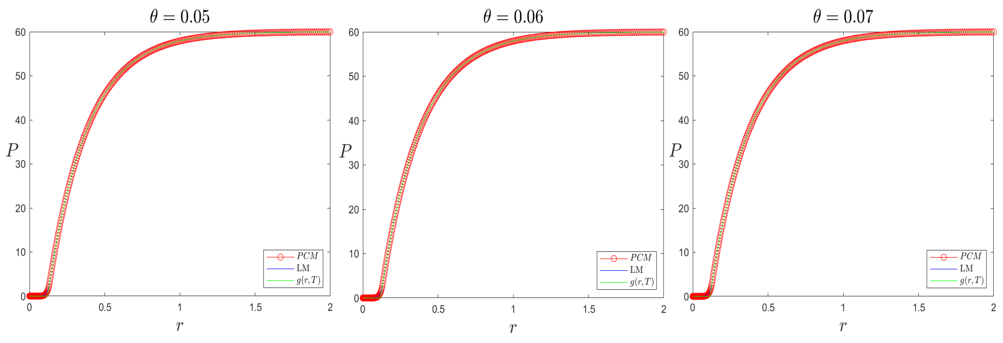
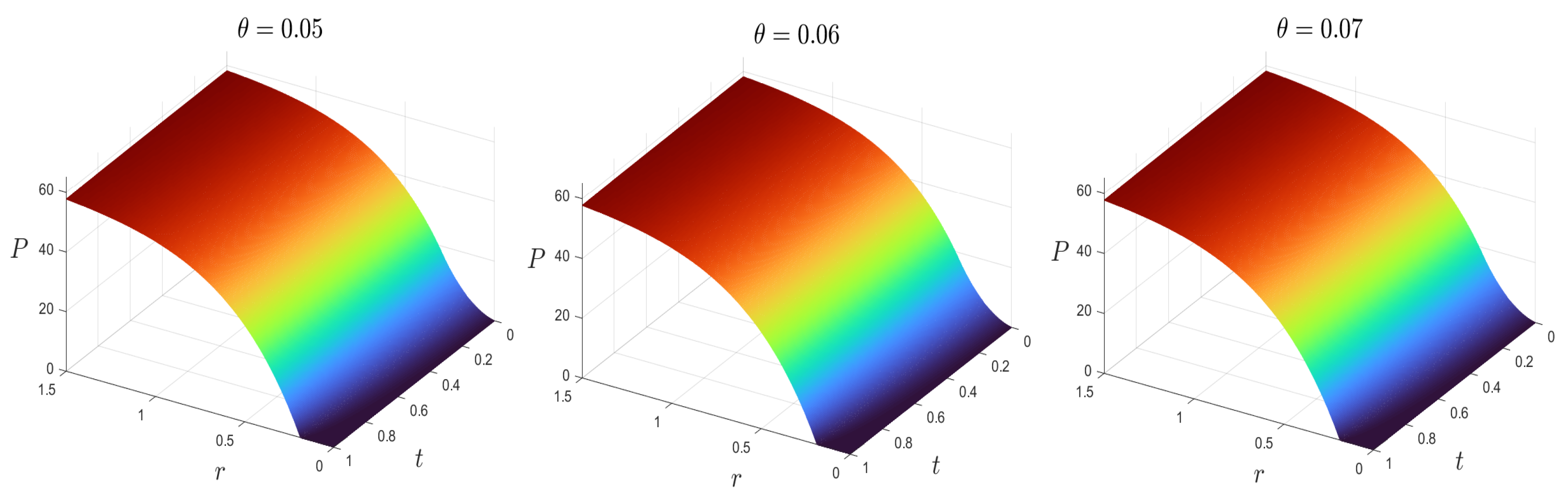
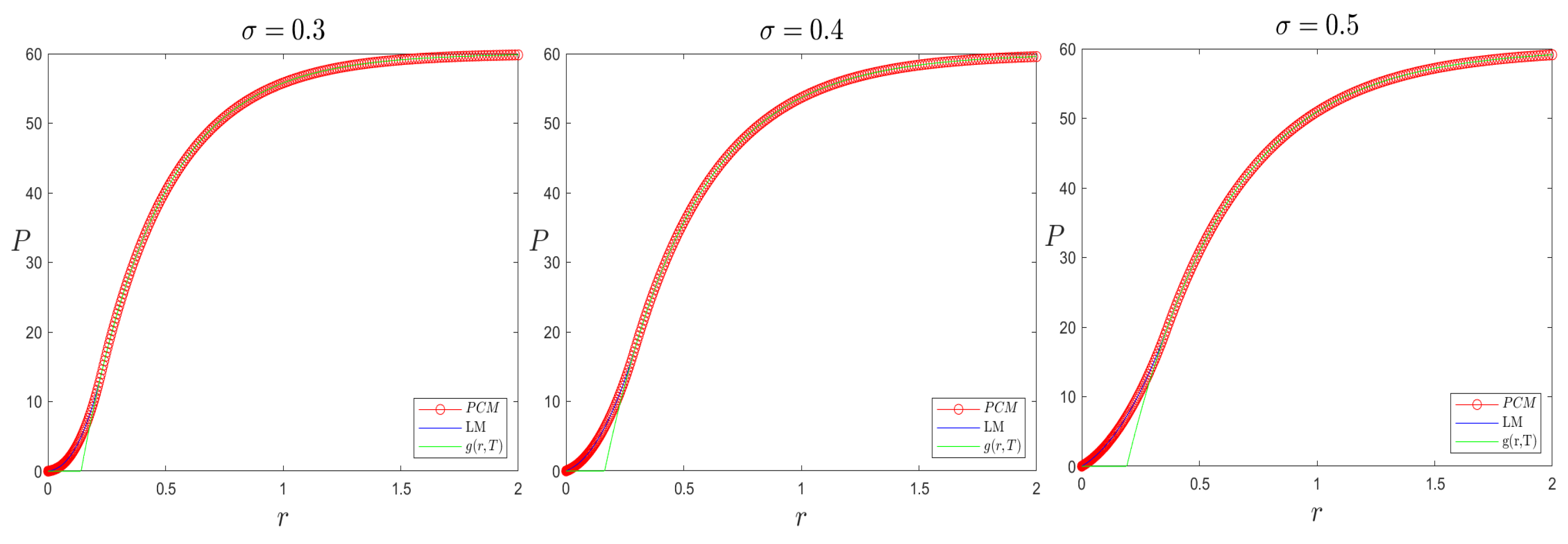
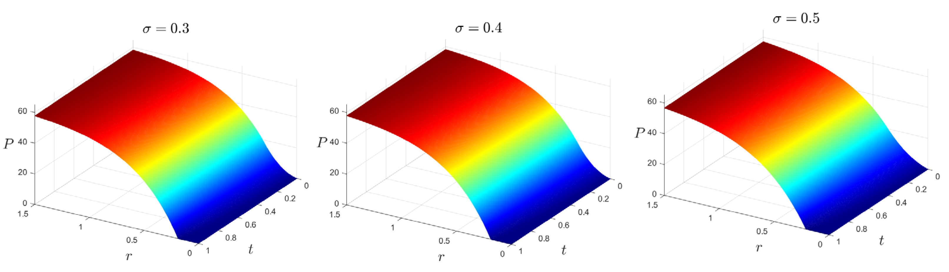
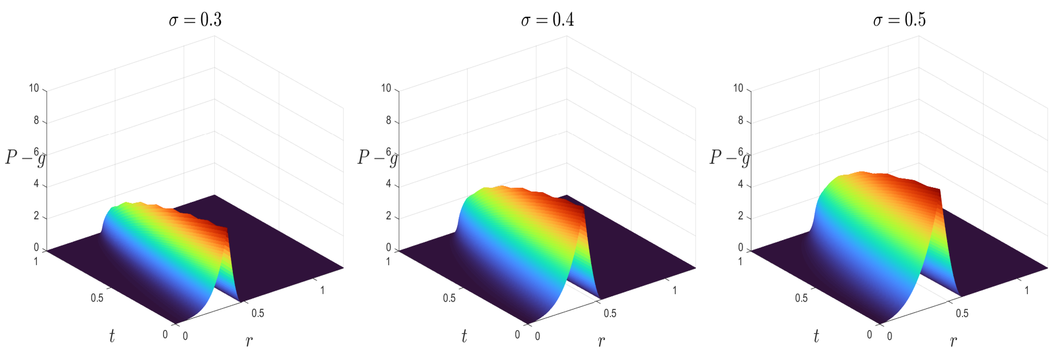
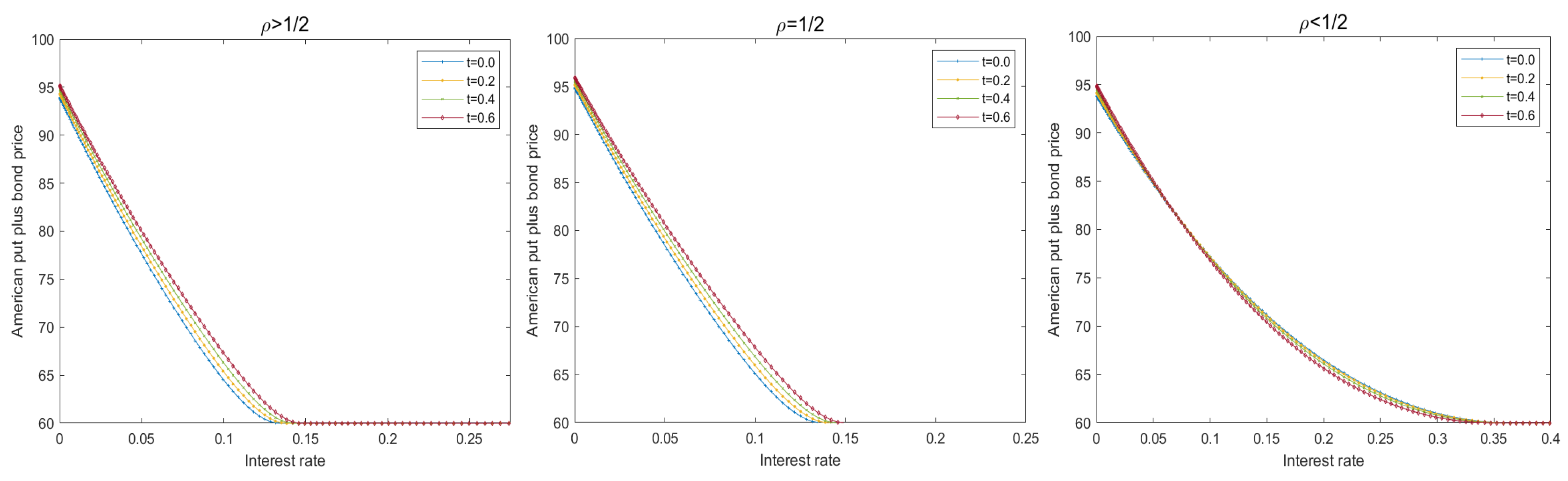
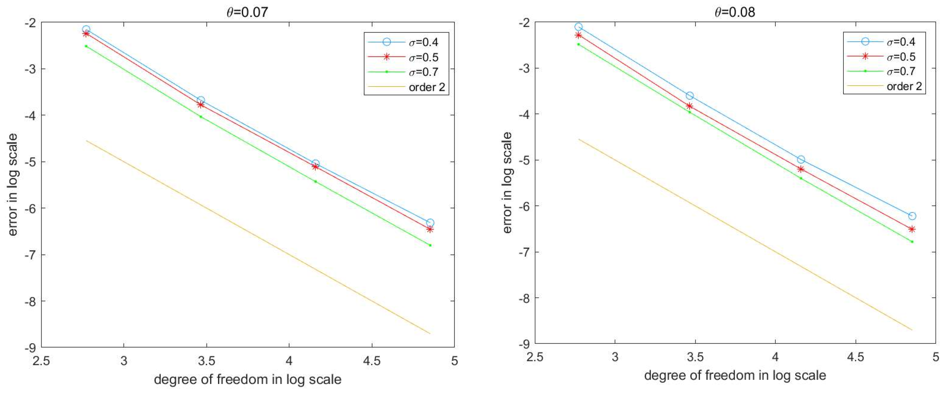
4. Numerical Simulation

In this section, we present some numerical examples to demonstrate the efficiency of the proposed method. Firstly, we give an example to verify the correctness of our algorithm by comparing it with the lattice method (LM) [28]. To give investors a better understanding of the American bond option pricing problem, we then provide several visual illustrations of options. Moreover, we give some numerical tests to indicate the validity of the projected and contraction method (PCM). Furthermore, we proposed some numerical tests to verify the error estimates. Finally, we give the numerical test to verify the fact that put price plus bond price is a decreasing function of $r$.

In the following examples, we mainly consider two special cases: Case I ($0<{\sigma }^2\le 2\kappa \theta$) and Case II ($2\kappa \theta <{\sigma }^2$), which can describe the validity of the algorithm. In addition, we consider the pricing problem of a one-year American zero-coupon bond option with a face value 100. The exercise price of the option is 60, i.e., $T=1,E=100,K=60$. The other parameters are chosen so that $\xi =0$, $s=5$, $R=2$ in all examples.

 Example 1.

In order to ensure the feasibility of the parameters, the parameters were chosen as those used in the literature [20]. We first consider Case I, where the model parameters satisfy the Feller condition. Parameter selection $\kappa =0.1$ and $\sigma =0.1$, we can change the value of $\theta$ to $0.05,0.06{,}_{}0.07{,}_{}$ when the feller condition is satisfied. We assume the LM with $M=5000$ as the reference solution and assume the PCM using time grid $M=600$ and space grid $N=300$. Figure 1 shows the values of $P(r,t)$ at time $t=0$ by LM and PCM for different $\theta$ values. The blue line represents the option price obtained using LM, the red line represents the option price obtained by PCM and the green line indicates the payoff function $g(r,T)$. Moreover, we present the three–dimensional image of the option prices $P(r,t)$ of the PCM against different values of $\theta$ in Figure 2.

Figure 1. Images of $P\left(r,0\right)$ for PCM and LM in different cases of $\theta$.

Figure 2. Three–dimensional images of the option value obtained by PCM.

In Figure 1 and Figure 2, we observed that the price of option $P(r,t)$ is an increasing function of $r$, which is consistent with the results in the literature [20]. And that the price obtained by PCM is nearly the same as the LM, which can verify the correctness of the proposed method. From Figure 2, we observe that the price trend of the option value is similar to standard American options.

 Example 2.

We consider the pricing problem for Case II with $\kappa =0.1$ and $\theta =0.08$. In order to examine the performance of our approach, we set the volatility $\sigma$at 0.3, 0.4 and 0.5.

In this example, we use numerical tests to verify the correctness of our method. Due to the lack of an analytical solution for American bond options, we use the LM with M = 5000 as the reference solution and assume the PCM using time grid $M=600$ and space grid $N=300$. Figure 3 shows the values of $P(r,t)$ at time $t=0$ by LM and PCM for different $\sigma$ values. The blue line represents the option price obtained using LM, the red line represents the option price obtained by PCM and the green line indicates the payoff function $g(r,T)$.

Figure 3. Images of $P\left(r,0\right)$ for PCM and LM in different cases of $\sigma$.

From Figure 3, it can be observed that the results obtained by the PCM are close to those obtained by the LM, and, in order to verify the proximity of the two methods, the error estimates and time consumption by the two methods are given in Table 1.

Table 1. Comparison of time consumption and error of LM and PCM.

	$\mathit{\sigma }=0.3$	$\mathit{\sigma }=0.4$	$\mathit{\sigma }=0.5$
LM $\left(s\right)$	46.52	34.81	27.78
PCM $\left(s\right)$	0.8139	1.0619	1.2536
Error $\left({10}^{-4}\right)$	1.4559	1.3267	1.2596

From Figure 3 and Table 1, it can be seen that the option price obtained by using the PCM is sufficiently close to the option price obtained by the LM, and the error of PCM reaches ${10}^{-4}$, which fully verifies the correctness of the PCM.

For a more intuitive understanding of the zero-coupon bond pricing problem, we can transform it into $P(r,T-\tau )=x^{-\alpha }{e}^{\beta \tau }u(x,\tau )$, Figure 4 represents a three–dimensional image of the option prices $P$ of the PCM against different values of $\sigma$.

Figure 4. Three–dimensional images of option value obtained by PCM.

As can be seen from the results, the trend of bond option prices is similar to that of standard American options, further justifying the proposed algorithm. The difference between the option value $P$ and payoff function $g(r,t)$ is represented by Figure 5.

Figure 5. The difference between the option value and payoff function.

 Example 3.

To demonstrate that our method is robust, we change the parameter $\theta =0.04{,}_{}0.06{,}_{}0.08$ in the Example 1.

In this example, we show that the computational speed of the PCM is comparable to the fitted finite volume method (FFVM) [30] whereas its accuracy is slightly better. The results obtained by the PCM are compared with those obtained by the LM and the FFVM, respectively, and the time spent and the error are presented in Table 2.

Table 2. Comparison of time consumption and error of FFVM and PCM.

$\mathit{\theta }$	0.04			0.06			0.08
$\mathit{\sigma }$	0.3	0.4	0.5	0.3	0.4	0.5	0.3	0.4	0.5
FFVM Error/${10}^{-4}$	2.06	1.56	1.36	2.03	1.64	1.40	2.24	1.72	1.44
PCM Error/${10}^{-4}$	1.74	1.32	1.27	1.51	1.46	1.33	1.83	1.46	1.33
FFVM Time/s	1.27	1.31	1.36	1.37	1.28	1.37	1.17	1.34	1.41
PCM Time/s	0.81	1.02	1.30	0.82	1.02	1.26	0.80	1.06	1.31

It is obvious that the PCM is an efficient numerical method for American bond options, compared with the FFVM from Table 2, it mainly reflects that: (1) comparing to the FFVM, the PCM is nearer the LM; (2) the PCM is faster than the FFVM under the same order of magnitudes.

At the end of this section, we show the relationship between the spatial numbers and the spatial error. Let the temporal numbers be $M=600$, which could guarantee that the space error is dominant. Moreover, due to the lack of an analytic solution for the American bond option pricing problem, we choose the PCM as the reference solution with $M=1000,N=2000$.

Here we need to point out that the error we used in the following tests indicated that:

$$Error=\sqrt{\frac{{\displaystyle \sum _{i=0}^N(P(x_i,0)-P^{*}(x_i,0))}}{N+1}}.$$

Now, the convergence results can be reflected for the difference combination {$\sigma$,$\theta$} in Figure 6.

Figure 6. The convergence rates in the spatial direction for difference combination {$\sigma$,$\theta$}.

From this figure, we can obviously see that the convergence rates in the spatial direction for the proposed method all approximate to the order 2.

 Example 4.

For the different cases of $\rho =\frac{\kappa \theta }{{\sigma }^2}$, we provide the American put price plus bond prices in Figure 7. From this figure, it is seen that the price is a monotonically decreasing function of $r$.

Figure 7. Images of American put plus bond prices.

5. Conclusions

This study investigates the numerical solution to the pricing problem of American bond options. By transforming the pricing model into a bounded forward simplification model through variable substitution, we discretize the model using the finite difference method. Based on the positive definiteness of the discretized matrix, we apply the PCM algorithm to solve the discrete system and obtain the option prices. Finally, the correctness and effectiveness of the PCM algorithm are verified through numerical experiments.

References

- Zaevski, T.S. Pricing discounted American capped options. Chaos Solitons Fractals 2022, 156, 111833. [Google Scholar] [CrossRef]
- Zaevski, T.S. Pricing cancellable American put options on the finite time horizon. J. Futures Mark. 2022, 42, 1284–1303. [Google Scholar] [CrossRef]
- Kifer, Y. Game options. Financ. Stoch. 2000, 4, 443–463. [Google Scholar] [CrossRef]
- Zaevski, T. Perpetual cancellable American options with convertible features. Mod. Stoch. Theory Appl. 2023, 10, 367–395. [Google Scholar] [CrossRef]
- Chuang, C. Valuation of perpetual strangles: A quasi-analytical approach. J. Deriv. 2013, 21, 64–72. [Google Scholar] [CrossRef]
- Repplinger, D. Pricing of Bond Options: Unspanned Stochastic Volatility and Random Field Models; Springer Science & Business Media: Berlin/Heidelberg, Germany, 2008. [Google Scholar]
- Deng, Z.C.; Yu, J.N.; Yang, L. An inverse problem arisen in the zero-coupon bond pricing. Nonlinear Anal. Real World Appl. 2010, 11, 1278–1288. [Google Scholar] [CrossRef]
- Black, F.; Scholes, M. The pricing of options and corporate liabilities. J. Political Econ. 1973, 81, 637–654. [Google Scholar] [CrossRef]
- Magnou, G.; Mordecki, E.; Sosa, A. Pricing bond options in emerging markets: A case study. J. Dyn. Games Am. Inst. Math. Sci. 2018, 51, 21–30. [Google Scholar] [CrossRef]
- Bekaert, G.; Engstrom, E.; Ermolov, A. Macro risks and the term structure of interest rates. J. Financ. Econ. 2021, 141, 479–504. [Google Scholar] [CrossRef]
- Wang, X.; Xie, D.; Jiang, J.; Wu, X.; He, J. Value-at-Risk estimation with stochastic interest rate models for option-bond portfolios. Financ. Res. Lett. 2017, 21, 10–20. [Google Scholar] [CrossRef]
- Merton, R.C. On the pricing of corporate debt: The risk structure of interest rates. J. Financ. 1974, 29, 449–470. [Google Scholar]
- Vasicek, O. An equilibrium characterization of the term structure. J. Financ. Econ. 1977, 5, 177–188. [Google Scholar] [CrossRef]
- Cox, J.C.; Ingersoll, J.E.; Ross, S.A. A Theory of the Term Structure of Interest Rates. Econometrica 1985, 53, 385–407. [Google Scholar] [CrossRef]
- Chan, K.C.; Karolyi, G.A.; Longstaff, F.A.; Sanders, A.B. An empirical comparison of alternative models of the short-term interest rate. J. Financ. 1992, 47, 1209–1227. [Google Scholar]
- Lorig, M.; Suaysom, N. Options on bonds: Implied volatilities from affine short-rate dynamics. Ann. Financ. 2022, 18, 183–216. [Google Scholar] [CrossRef]
- Tomas, M.J.; Yu, J. An Asymptotic Solution for Call Options on Zero-Coupon Bonds. Mathematics 2021, 9, 1940. [Google Scholar] [CrossRef]
- Babbel, D.F.; Merrill, C.; Zacharias, J. Teaching Interest Rate Contingent Claims Pricing. J. Financ. Educ. 1996, 22, 41–59. [Google Scholar]
- Ho, T.S.; Stapleton, R.C.; Subrahmanyam, M.G. The valuation of American options on bonds. J. Bank. Financ. 1997, 21, 1487–1513. [Google Scholar] [CrossRef]
- Yang, H. American put options on zero-coupon bonds and a parabolic free boundary problem. Int. J. Numer. Anal. Model. 2004, 1, 203–215. [Google Scholar]
- Zhang, K.; Wang, S. Pricing American bond options using a penalty method. Automatica 2012, 48, 472–479. [Google Scholar] [CrossRef]
- Hilal, K.; Serghini, A. Pricing American bond options using a cubic spline collocation method. Bol. Soc. Parana. 2014, 32, 189–208. [Google Scholar]
- Gang, X.T.; Yi, H. A New Efficient Numerical Method for Pricing American Options on Zero-coupon Bonds. J. Eng. Math. 2021, 38, 879–900. [Google Scholar]
- Chesney, M.; Elliott, R.J.; Gibson, R. Analytical solutions for the pricing of American bond and yield options. Math. Financ. 1993, 3, 277–294. [Google Scholar] [CrossRef]
- Hao, X.N. A differential method to the American bond option pricing problem. J. Taiyuan Univ. Technol. 2008, 39, 137–144. [Google Scholar]
- He, B.S. A new method for a class of linear variational inequalities. Math. Program. 1994, 66, 137–144. [Google Scholar] [CrossRef]
- Song, H.M.; Zhang, R. Projection and contraction method for the valuation of American options. East Asian J. Appl. Math. 2015, 5, 48–60. [Google Scholar] [CrossRef]
- Tian, Y.S. A reexamination of lattice procedures for interest rate-contingent claims. Adv. Futures Options Res. 1994, 7, 87–111. [Google Scholar]
- Allegretto, W.; Lin, Y.; Yang, H. Numerical pricing of American put options on zero-coupon bonds. Appl. Numer. Math. 2003, 46, 113–134. [Google Scholar] [CrossRef]
- Wilmott, P.; Howison, S.; Dewynne, J. The Mathematics of Financial Derivatives: A Student Introduction; Cambridge University Press: Cambridge, UK, 1995. [Google Scholar]
- Wang, S. A novel fitted finite volume method for the Black–Scholes equation governing option pricing. IMA J. Numer. Anal. 2004, 24, 699–720. [Google Scholar] [CrossRef]
Disclaimer/Publisher’s Note: The statements, opinions and data contained in all publications are solely those of the individual author(s) and contributor(s) and not of MDPI and/or the editor(s). MDPI and/or the editor(s) disclaim responsibility for any injury to people or property resulting from any ideas, methods, instructions or products referred to in the content. |
© 2023 by the authors. Licensee MDPI, Basel, Switzerland. This article is an open access article distributed under the terms and conditions of the Creative Commons Attribution (CC BY) license (https://creativecommons.org/licenses/by/4.0/).