Abstract
This paper considers the fixed-time synchronization of complex-valued coupled networks (CVCNs) with hybrid perturbations (nonlinear bounded external perturbations and stochastic perturbations). To accomplish the target of fixed-time synchronization, the CVCNs can be separated into their real and imaginary parts and establish real-valued subsystems, a novel quantized controller is designed to overcome the difficulties induced by complex parameters, variables, and disturbances. By means of the Lyapunov stability theorem and the properties of the Wiener process, some sufficient conditions are presented for the selection of control parameters to guarantee the fixed-time synchronization, and an upper bound of the setting time is also obtained, which is only related to parameters of both systems and the controller, not to the initial conditions of the systems. Finally, a numerical simulation is given to show the correctness of theoretical results and the effectiveness of the control strategy.
Keywords:
complex-valued coupled networks; fixed-time synchronization; hybrid perturbations; quantized control MSC:
35R60; 60H15; 35A01
1. Introduction
The dynamical behaviors of real-valued neural networks (RVNNs) have been widely studied in diverse areas such as biology, information processing, and secure communications [1,2,3]. Compared with RVNNs, complex-valued neural networks (CVNNs) have attracted much attention because of their wide application in nonlinear filtering [4], optoelectronics [5], computer vision [6], remote sensing [7], and synthesis [8], in view of their greater computing power and information storage capabilities. In addition, they have been applied to describe wave functions in quantum mechanics and calculate parameters such as the voltage, current, and power in alternating current circuits [9,10]. At present, the study of CVCNs has involved many aspects, such as stability [11,12], bifurcation [13], and synchronization [14]. Therefore, we investigate the dynamics of CVCNs. Synchronization is a very peculiar phenomenon where the dynamic signals of chaotic systems converge to identical behavior over time.
Since the concept of synchronization was first proposed by Pecora and Carroll [15], many researchers have investigated this hot topic, and many different synchronization types have been introduced, such as asymptotic synchronization [16,17], exponential synchronization [14,18,19,20], finite-time synchronization [21,22,23,24,25,26,27,28,29], and so on.
It should be noted that asymptotic and exponential synchronization can be achieved as time approaches infinity. However, when considering real-world applications influenced by uncertain factors, achieving infinite time synchronization of the systems is not conducive to secure communication. Therefore, in order to improve the security of communication, it is important to accomplish synchronization within a certain finite time, namely finite-time synchronization. In addition, due to the fast convergence speed, finite-time synchronization is a good choice, which can ensure better robustness and anti-interference. For finite-time synchronization, in order to estimate the synchronization setting time, the initial value conditions of the systems are needed. However, from a practical point of view, it is difficult to obtain initial value conditions of the networks, limiting the applications of the finite-time technique. Recently, the fixed-time technique, as a special case of the finite-time technique, was proposed [30]. The advantage of the fixed-time technique is that the synchronization setting times only relate to the parameters of the systems, independent of the initial conditions. Thus, with the aid of the fixed-time technique, many excellent results were presented. In [31,32], fixed-time synchronization of RVNN was studied. The synchronization of complex networks under a fixed-time technique was investigated in [33,34]. The fixed-time synchronization of CVNNs was considered in [35,36,37].
The control strategy plays an important role in the framework of the fixed-time control technique. Thus, the designed controllers should be easy to implement in practice and reduce the control costs as much as possible. In [35,36,37,38,39], the synchronization of complex-valued networks was studied by state feedback control with precise error signals. However, when the network is frequently disturbed by external factors due to unknown factors in the real world, the transmitted signal can become very weak. In addition, due to the limitation of information transmission channels and bandwidth, communication constraints will be encountered. Therefore, it is very difficult to obtain accurate error information from practical applications. Recently, since the quantizer can quantize the signals with restricted information before transmission, the quantification technique has been widely used to achieve the control goals. Compared with the control strategy presented in [35,36,37,38,39], quantitative control is more regnant. The synchronization of neural networks via quantized output control was studied in [19,20,40]. In [23], the stabilization for a class of switched dynamical networks in finite time was investigated by a quantification technique. In [41], the authors investigated cluster synchronization of neural networks within a finite timeframe by crafting new non-chattering quantized controllers. In [42], research was conducted on the finite-time synchronization of quantized Markovian-jump time-varying delayed neural networks, with the design centered on an event-triggered control scheme. It is worth noting that the above works focus on the synchronization of real-valued systems, and there is no relevant literature on the fixed-time synchronization of CVCNs using quantized control.
Because there are certain unknown factors in the environment, it is inevitable that the CVCNs are often disturbed, and these disturbances can lead to more complex dynamic behaviors in the network. Therefore, the study of networks with disturbances is more significant in practical applications. On the one hand, some random fluctuations produced in the process of information transmission can be denoted as random perturbations. At present, there are numerous works on stochastic perturbations [17,19,33,35,38,43]. In particular, the synchronization of complex variable chaotic systems with stochastic perturbations via adaptive control was studied in [17]. The fixed-time synchronization of stochastic complex-valued fuzzy neural networks was investigated in [35]. Nonlinear perturbations should also be taken into account for networks due to environmental factors. In addition, artificially adding nonlinear interference to the network can improve the message transmission security. For example, the finite-time synchronization of chaotic systems with nonidentical perturbations was investigated in [22,24,25]. It should be noted that only infinite time synchronization can be achieved in [17,38], and either random perturbations or nonlinear bounded external perturbations were considered in [22,24,35]. Overcoming the effects of random and nonlinear perturbations is more difficult than considering one or the other. To our understanding, few researchers have considered the fixed-time synchronization of CVCNs with random and nonlinear perturbations. Moreover, the received signal is weak when the information carrier system suffers from external disturbances; the control strategy in [17,22,24,25,38] cannot be directly applied to achieve synchronization. For this purpose, this paper aims to solve this challenging and significant problem via a suitable quantization controller.
Inspired by the above discussion, in this paper, we consider the fixed-time synchronization CVCNs with mixed perturbations (i.e., stochastic disturbances and nonlinear bounded external disturbances). Since the mixed perturbations are taken into account and the parameters of the slave system differ from those of the master system, the master system is more practical than the system in [21,22,27,38]. The control strategies proposed in this paper are more general than those in [35,36,37,38,39].
The main contributions are as follows. Based on the advantage of a quantizer, a new quantized control method is proposed to further save communication resources and reduce control costs. Moreover, even though the received signal is weak, the target of fixed-time synchronization can be achieved under the design control strategy. The designing controller can simultaneously overcome the difficulties induced by complex parameters, variables, and disturbances, and it has better robustness and disturbance rejection. Several sufficient conditions are obtained to guarantee fixed-time synchronization, considering CVCNs. Compared with the literature [17,22,38,39], due to the practicability of the system and the superiority of the control strategy, the results of this paper have strong universality.
The organization of this paper is as follows: In Section 2, the model consisting of CVCNs with hybrid perturbations is proposed. Some necessary definitions, assumptions, and lemmas are also presented. In Section 3, the fixed-time synchronization of the CVCNs considered is studied. In Section 4, a numerical simulation is given to show the correctness of theoretical results and the effectiveness of the control strategy. In Section 5, the conclusion is provided.
Notations: denotes a set of n-dimensional complex vectors. For , and denote the real and imaginary parts of x, respectively, . is the Euclidean norm, and denotes the n-dimensional Euclidean space. The superscript T denotes the transposition of a matrix or vector. is the identity matrix. means the largest eigenvalue of A, . Moreover, let be a complete probability space with filtration satisfying the usual conditions (i.e., the filtration contains all P-null sets and is right-continuous). We denote by the family of all -measurable -valued random variables , such that , where stands for the mathematical expectation operators, with respect to the given probability measure P.
2. Model Description and Some Preliminaries
Considering the interactions among multiple neural networks, the coupled complex-valued system is composed of N nodes, and each node contains two different perturbations; the dynamic evolution of the CVCNs with hybrid perturbations is described by
with the initial condition
where represents the n-dimensional complex-valued state vector of the ith node with , , , and are real and imaginary parts of , respectively, represents the self-feedback connection weight, is a nonlinear complex-valued vector function, describes the inner coupling matrix of the network, and is the linear coupling matrix; it represents the topology configuration of the entire network, satisfying if there is a connection between nodes i and j, otherwise, . Moreover, the diagonal elements of matrix A are defined as . In addition, represents nonlinear external bounded perturbations, is the noise intensity function matrix, and is a vector-form Wiener process defined on a complete probability space . is a control input that will be designed later.
Consider the CVCNs (1) as the master system; the slave system is described by
where represents the n-dimensional complex-valued state vector of the slave system (2), the definitions of , and are similar to those of system (1). In addition, the initial value of system (2) is .
In the following, we state the definition of fixed-time synchronization and present some lemmas.
Definition 1
([33]). The master system (1) is said to be synchronized with the slave system (2) within a fixed time, if there exists , which is independent of the initial value , , such that
for , where is called the setting time.
Let , subtracting (2) from (1), then the error system is described by
with initial condition , where , . Let , , , , , . Then the error system (3) can be separated into real and imaginary parts, as
with the initial condition
Remark 1.
In order to establish the main results, in the following, we present some assumptions.
Assumption 1.
Positive constants exist, , such that , where
Assumption 2.
Assumption 3.
Nonnegative constants— and —exist, such that
In order to better achieve the objectives of this article, we present some properties of the Wiener processes [17,26].
(1) ;
(2) For , is a scalar function. We can obtain the differential equation’s V differential form as follows
Lemma 1
([30]). If a continuous radially unbounded function exists, , such that
- (1)
- ;
- (2)
- for , , , any solution satisfies the following inequality:then the origin of the network is globally stable in fixed-time equilibrium, and the fixed settling time is given by .
Lemma 2
([44]). Let and . Then the following two inequalities hold:
3. Fixed-Time Synchronization of CVCNs
To discuss the fixed-time synchronization of the master–slave systems (1) and (2) described in Section 2, in this section, we extend the controller method in [20,41] and design a suitable quantification controller as follows:
where , , and are positive constants to be determined later, and , , , are tunable constants. , , . The from of is the same as , is a quantizer, where with . For , the quantizer is defined as follows:
where . According to the Filippov regularization in [45], there exists a Filippov solution , such that ; since , it is obvious to obtain and .
Remark 2.
In [35,37], the fixed-time synchronization of complex-valued chaotic systems was investigated by designing the state feedback control. Note that the continuity and precisely state signal are needed for the state feedback controller. However, from a practical of view, it is quite difficult to receive precision signs due to the limitations of the information transmission channel and bandwidth. Therefore, the quantification control strategy is more practical than the controller in [20,41]. Moreover, the controller (5) can save the resources of the channel and reduce control costs.
Remark 3.
In order to better understand the quantization controller, the following explanation is needed. The quantization process is based on the quantizer to convert the received signal of the continuous change in time and amplitude into a digital signal. According to the definition of , for any given , , it is easy to see that
(1) if the received signal , then ;
(2) if the received signal , and with , and , then (a) for , we have ; (b) for , we have ;
(3) if the received signal , and with and , then (a) for , we have ; (b) for , we have .
Moreover, if and , then . If and , then . Thus, there exists a Filippov solution , such that .
In the following, some sufficient conditions are derived to achieve the fixed-time synchronization of the master–slave systems (1) and (2).
Theorem 1.
The master system (1) can be synchronized with the slave system (2) in a fixed time if Assumption 1–3 and the following conditions are satisfied:
where , , , is the minimum eigenvalue of ; , , , , , , . Moreover, the setting time is estimated as
Proof.
Consider the Lyapunov function as follows:
According to the properties of the Wiener process in [17,26], differentiating along the solution of the error system (4), one obtains that
Taking the expectations on both sides of Equation (9), then applying (4) and Assumption 3, we have
It can be obtained from Assumption 1 that
and
Applying (11) and (12), we can obtain
Applying (4) and Assumption 2, we can obtain
and
Applying (5), we have the following estimates:
and
where . Substituting (11)–(17) into (10) yields
where
It can be obtained from Lemma 2 that
and
From (18)–(20), one can obtain
Therefore, according to Lemma 1, the solution of system (4) is stable in fixed time, which means that system (1) is synchronized with (2) under the controller (5). Moreover, the setting time is estimated as
The proof is completed. □
Remark 4.
From the proof of Theorem 1, we can see that the discontinuous terms and in controller (5) play an important role in realizing the fixed-time synchronization. The inequalities (14) and (15) show that these terms can overcome the effects of complex parameters, variables, and nonlinear-bounded external disturbances. However, the system parameters are identical, without considering both stochastic disturbances and nonlinear perturbations simultaneously in [36,37]. Therefore, our results are more general than those in [36,37].
Remark 5.
Although there are many literature studies that study the synchronization of chaotic systems, there is no work on the fixed-time synchronization of complex-valued chaotic systems with double perturbations. In [28,29,39], the finite-time synchronization of complex-valued chaotic systems is discussed, and the control techniques of these papers cannot be directly applied to realize fixed-time synchronization. Although references [35,36,37] also studied the fixed time synchronization of complex-valued chaotic systems, the system in [35] only considered random perturbations. Therefore, our results derived here can be extended to more general systems to achieve finite-time synchronization and fixed-time synchronization.
In the following, we present two special cases.
Case 2: All the nodes of system (1) are identical with the isolated node of system (2), i.e., , . Then Corollary 1 and 2 can be obtained from Theorem 1.
Corollary 1.
Suppose that , and Assumption 1–3 hold, then the system (1) can be synchronized with (2) in fixed time if the control parameters in (5) are chosen to satisfy
where , , the other parameters are defined as those in Theorem 1.
Corollary 2.
Suppose that , , and Assumption 1–3 hold, then the system (1) can be synchronized with (2) in fixed time if the control parameters in (5) are chosen to satisfy
where the other parameters are defined as those in Theorem 1.
Remark 6.
By lemma 1, inequality (19) and (20) show that the terms of and in (5) plays a key role in investigating fixed-time synchronization. The setting time entirely depends on the tunable parameters of these terms and the dimensions of CNs, meaning that the setting time can be pre-designed. From a practical of view, faster convergence and improved security of communication can be guaranteed based on Theorem 1, as well as Corollaries 1 and 2.
Remark 7.
Corollaries 1 and 2 show that the fixed-time synchronization of the coupled networks is also achieved when parameters C and of system (1) are real and the state variables are complex. More generally, if parameters η and ζ are zeros, then the asymptotic synchronization of coupled networks with complex-valued state variables can be obtained. Thus, the synchronization criteria in [17] are a special case of those discussed in this paper.
4. Simulation
In this section, an example is given to show the correctness of the theoretical results and the effectiveness of the control strategy.
Example 1.
In the following, we consider two types of complex-valued nodes. One is described as
where , , and
We take the initial conditions as , the corresponding state trajectories of real and imaginary parts for system (22) are shown in Figure 1a,b. From Figure 1, it is clear that system (22) is chaotic. Moreover, the states are bounded with , , , , , and .
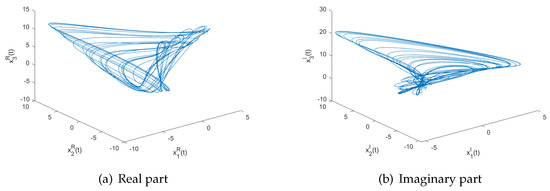
Figure 1.
Chaotic trajectory of system (22) with the initial value .
The other system with the slave system is described by
where , and
We take the initial conditions as , the corresponding state trajectories of the real and imaginary parts for system (23) are chaotic in Figure 2a,b. Moreover, the states are bounded with , , , , , and .
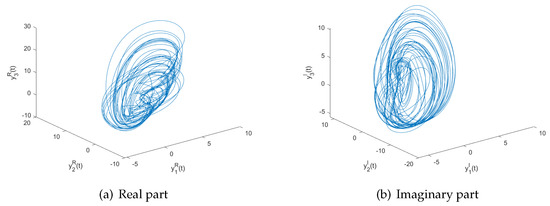
Figure 2.
Chaotic trajectory of system (23) with the initial value .
We consider a complex-valued coupled system composed of system (22) with 5 nodes as the master system; it is described by
where , , the nonlinear bound external perturbations
the noise intensity function matrix
and the outer coupling matrix
By a simple calculation, it is easy to see that , , , , . Then we can obtain
and
Thus, the results of Assumption 1 are met. In addition, we have the following results from (24)
and
Thus, the Assumption 3 is met. Moreover, Assumption 2 is also met with , , , , , , , , , , .
Now we embark on the fixed-time synchronization of the master–slave system (24) and (23). We take , , , , , , , , , . Moreover, we choose parameters , , , and the time-step size is 0.0001 in the simulation computation. According to Theorem 1, the fixed-time synchronization of the master–slave system (24) and (23) is reached with the controller (5), and the setting time in Figure 3. Moreover, the quantized error trajectories are also shown in Figure 4. From a numerical experiment, it can be directly observed that the numerical conclusions affirm Theorem 1.
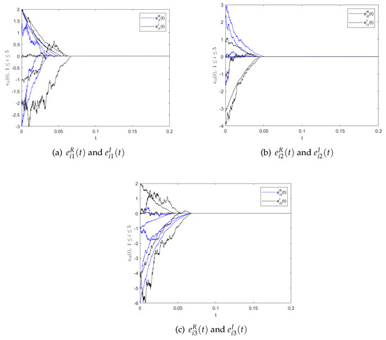
Figure 3.
The time response of synchronization errors and , .
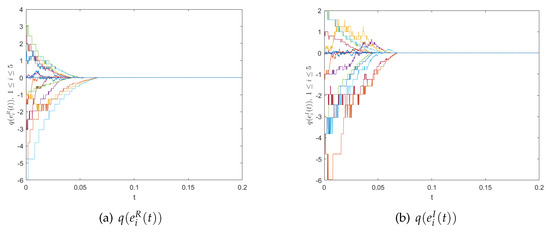
Figure 4.
The time response of quantized error trajectories.
In order to verify that the synchronization setting times are independent of the initial conditions, in the following, we present two additional sets of initial conditions and plot the time responses of the corresponding synchronization errors, respectively. The results obtained are compared with Figure 3. We take the initial conditions and , where the states are bounded with , , , , , , and , , , , and . Figure 5 shows the time response of the synchronization error trajectories with control gains , , , , and the setting time . The other set of parameters is as follows. We take the initial conditions , and , where the states are bounded with , , , , , , and , , , , , and . Figure 6 shows the time responses of synchronization error trajectories with control gains , , , and the setting time . Therefore, from the results of Figure 3, Figure 5, and Figure 6, it is easy to see that the synchronization setting time is independent of the initial value conditions.
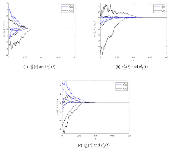
Figure 5.
The time responses of synchronization errors and , .
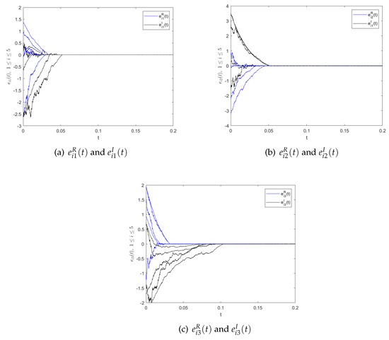
Figure 6.
The time responses of synchronization errors and , .
5. Conclusions
In this paper, we studied the synchronization for CVCNs with both stochastic disturbances and nonidentical bounded external disturbances in fixed time. To achieve fixed-time synchronization, we designed a novel quantized controller, which can restrict the effects of complex parameters, variables, and disturbances. Based on the framework of the Lyapunov stability theorem and the properties of the Wiener process, several synchronization criteria were obtained, and the settling time was estimated. Some existing results on the fixed-time synchronization of CVCNs were extended. Numerical simulations verify the correctness of the theoretical results and the effectiveness of the control strategy.
In this paper, we considered only the fixed-time synchronization of CVCNs with double disturbances in order to reduce the computational difficulties. But in real applications, many systems are affected by several different factors. Thus, in future work, we plan to investigate finite-time synchronization and fixed-time synchronization under many different kinds of disturbances by designing a suitable controller, which is important and interesting, but much more difficult.
Author Contributions
E.W.: investigation, methodology, validation, data curation, software, writing—original draft. Y.W.: investigation, methodology, data curation. Y.L.: investigation, software, data duration. K.L.: investigation, methodology, validation. F.L.: conceptualization, investigation, methodology, validation, data duration, writing—reviewing and editing. All authors have read and agreed to the published version of the manuscript.
Funding
This work is supported by the National Natural Science Foundation of China (grant nos. 11971019 and 61573010), the Opening Project of the Sichuan Province University Key Laboratory of Bridge Non-destruction Detecting and Engineering Computing (grant nos. 2022QZJ02, 2021QYJ03 and 2020QYJ03), the National Natural Science Foundation of Sichuan (grant no. 2023NSFSC1021).
Institutional Review Board Statement
Not applicable.
Informed Consent Statement
Not applicable.
Data Availability Statement
Not applicable.
Conflicts of Interest
The authors declare no conflict of interest.
References
- Liao, T.; Huang, N. An observer-based approach for chaotic synchronization with applications to secure communications. IEEE Trans. Circuits Syst. I 1999, 46, 1144–1150. [Google Scholar] [CrossRef]
- Strogatz, H.S.; Stewart, I. Coupled oscillators and biological synchronization. Sci. Amer. 1993, 269, 102–109. [Google Scholar] [CrossRef]
- Abeles, M.; Prut, Y.; Bergman, H.; Vaadia, E. Synchronization in neuronal transmission and its importance for information processing. Prog. Brain Res. 1994, 102, 395–404. [Google Scholar] [PubMed]
- Cha, I.; Kassam, S.A. Channel equalization using adaptive complex radial basis function networks. IEEE J. Sel. Area. Comm. 1995, 13, 122–131. [Google Scholar]
- Chen, S.; Hanzo, L.; Tan, S. Symmetric complex-valued rbf receiver for multiple-antenna-aided wireless systems. IEEE Trans. Neural Netw. 2008, 19, 1659–1665. [Google Scholar] [CrossRef] [PubMed][Green Version]
- Kim, T.; Adali, T. Fully complex multi-layer perceptron network for nonlinear signal processing. J. Vlsi Signal Process. 2002, 32, 29–43. [Google Scholar] [CrossRef]
- Nitta, T. Orthogonality of decision boundaries in complex-valued neural networks. Neural Comput. 2004, 16, 73–97. [Google Scholar] [CrossRef] [PubMed]
- Tanaka, G.; Aihara, K. Complex-valued multistate associative memory with nonlinear multilevel functions for gray-level image reconstruction. IEEE Trans. Neural Netw. 2009, 20, 1463–1473. [Google Scholar] [CrossRef]
- Wu, K.; Kondra, T.V.; Rana, S.; Scandolo, C.M.; Xiang, G.; Li, C.; Guo, G.; Streltsov, A. Resource theory of imaginarity: Quantification and state conversion. Phys. Rev. A 2021, 103, 032401. [Google Scholar] [CrossRef]
- Canay, I.M. Modelling of alternating-current machines having multiplt rotor circuits. IEEE Trans. Energy Convers. 1993, 2, 280–296. [Google Scholar] [CrossRef]
- Liang, J.; Gong, W.; Huang, T. Multistability of complex-valued neural networks with discontinuous activation functions. Neural Netw. 2016, 84, 125–142. [Google Scholar] [CrossRef] [PubMed]
- Velmurugan, G.; Rakkiyappan, R.; Cao, J. Further analysis of global μ-stability of complex-valued neural networks with unbounded time-varying delays. Neural Netw. 2015, 67, 14–27. [Google Scholar] [CrossRef] [PubMed]
- Huang, C.; Cao, J.; Xiao, M.; Alsaedi, A.; Hayat, T. Bifurcations in a delayed fractional complex-valued neural networks. Appl. Math. Comput. 2017, 292, 210–227. [Google Scholar] [CrossRef]
- Bao, H.; Park, J.H.; Cao, J. Exponential synchronization of coupled stochastic memristor-based neural networks with time-varying probabilistic delay coupling and impulsive delay. IEEE Trans. Neural Netw. 2016, 27, 190–201. [Google Scholar] [CrossRef] [PubMed]
- Pecora, L.M.; Carrol, T.L. Synchronization in chaotic systems. Phys. Rev. Lett. 1990, 64, 821–824. [Google Scholar] [CrossRef] [PubMed]
- Yang, Z.; Luo, B.; Liu, D.; Li, Y. Pinning synchronization of memristor-based neural networks with time-varying delays. Neural Netw. 2017, 93, 143–151. [Google Scholar] [CrossRef]
- Wu, E.; Yang, X. Adaptive synchronization of coupled nonidentical chaotic systems with complex variables and stochastic perturbations. Nonlinear Dyn. 2016, 84, 261–269. [Google Scholar] [CrossRef]
- Wang, G.; Yin, Q.; Shen, Y. Exponential synchronization of coupled fuzzy neural networks with disturbances and mixed time-delays. Neurocomputing 2013, 106, 77–85. [Google Scholar] [CrossRef]
- Zhang, W.; Yang, S.; Li, C.; Zhang, W.; Yang, X. Stochastic exponential synchronization of memristive neural networks with time-varying delays via quantized control. Neural Netw. 2018, 104, 93–103. [Google Scholar] [CrossRef]
- Yang, X.; Cheng, Z.; Li, X.; Ma, T. Exponential synchronization of coupled neutral-type neural networks with mixed delays via quantized output control. J. Frankl. Inst. 2019, 356, 8138–8153. [Google Scholar] [CrossRef]
- Zhang, C.; Wang, X.; Unar, S.; Wang, Y. Finite-time synchronization of a class of nonlinear complex-valued networks with time-varying delays. Phys. A 2019, 528, 120985. [Google Scholar] [CrossRef]
- Luo, F.; Xiang, Y.; Wu, E. Finite-time synchronization of coupled complex-valued chaotic systems with time-delays and bounded perturbations. Mod. Phys. Lett. B 2022, 35, 2150130. [Google Scholar] [CrossRef]
- Yang, X.; Cao, J.; Xu, C.; Feng, J. Finite-time stabilization of switched dynamical networks with quantized couplings via quantized controller. Sci. China Technol. Sci. 2018, 61, 299–308. [Google Scholar] [CrossRef]
- Shi, L.; Yang, X.; Li, Y.; Feng, Z. Finite-time synchronization of nonidentical chaotic systems with multiple time-varying delays and bounded perturbations. Nonlinear Dyn. 2016, 83, 75–87. [Google Scholar] [CrossRef]
- Yang, X.; Wu, Z.; Cao, J. Finite-time synchronization of complex networks with nonidentical discontinuous nodes. Nonlinear Dyn. 2010, 73, 2313–2327. [Google Scholar] [CrossRef]
- Yang, X.; Cao, J. Finite-time stochastic synchronization of complex networks. Appl. Math. Model. 2010, 34, 3631–3641. [Google Scholar] [CrossRef]
- Xiong, K.; Yu, J.; Hu, C.; Jiang, H. Synchronization in finite/fixed time of fully complex-valued dynamical networks via nonseparation approach. J. Frankl. Inst. 2020, 357, 473–493. [Google Scholar] [CrossRef]
- Zhang, Z.; Li, A.; Yu, S. Finite-time synchronization for delayed complex-valued neural networks via integrating inequality method. Neurocomputing 2018, 318, 248–260. [Google Scholar] [CrossRef]
- Sun, K.; Zhu, S.; Wei, Y.; Zhang, X.; Gao, F. Finite-time synchronization of memristor-based complex-valued neural networks with time delays. Phys. Lett. A 2019, 383, 2255–2263. [Google Scholar] [CrossRef]
- Polyakov, A. Nonlinear feedback design for fixed-time stabilization of linear control systems. IEEE Trans. Autom. Control 2012, 57, 2106–2110. [Google Scholar] [CrossRef]
- Wan, Y.; Cao, J.; Wen, G.; Yu, W. Robust fixed-time synchronization of delayed cohen-grossberg neural networks. Neural Netw. 2016, 73, 86–94. [Google Scholar] [CrossRef] [PubMed]
- Cao, J.; Li, R. Fixed-time synchronization of delayed memristor-based recurrent neural networks. Sci. China Inf. Sci. 2017, 60, 032201. [Google Scholar] [CrossRef]
- Zhang, W.; Yang, X.; Li, C. Fixed-time stochastic synchronization of complex networks via continuous control. IEEE Trans. Cybern. 2019, 49, 3099–3104. [Google Scholar] [CrossRef] [PubMed]
- Yang, X.; Lam, J.; Ho, D.W.C.; Feng, Z. Fixed-Time synchronization of complex networks with impulsive effects via nonchattering control. IEEE Trans. Autom. Control 2017, 99, 5511–5521. [Google Scholar] [CrossRef]
- Wang, P.; Li, X.; Lu, J.; Lou, J. Fixed-time synchronization of stochastic complex-valued fuzzy neural networks with memristor and proportional delays. Neural Process. Lett. 2023. [CrossRef]
- Feng, L.; Hu, C.; Yu, J.; Jiang, H.; Wen, S. Fixed-time synchronization of coupled memristive complex-valued neural networks. Chaos Solitons Fractals 2021, 148, 110993. [Google Scholar] [CrossRef]
- Ding, X.; Cao, J.; Alsaedi, A.; Alsaadi, F.E.; Hayat, T. Robust fixed-time synchronization for uncertain complex-valued neural networks with discontinuous activation functions. Neural Netw. 2017, 90, 42–55. [Google Scholar] [CrossRef] [PubMed]
- Wang, P.; Jin, W.; Su, H. Synchronization of coupled stochastic complex-valued dynamical networks with time-varying delays via aperiodically intermittent adaptive control. Chaos 2018, 28, 043114. [Google Scholar] [CrossRef]
- Zhang, C.; Wang, X.; Wang, S.; Zhou, W.; Xia, Z. Finite-time synchronization for a class of fully complex-valued networks with coupling delay. IEEE Access 2018, 6, 17923–17932. [Google Scholar] [CrossRef]
- Zhang, W.; Li, C.; Yang, S.; Yang, X. Synchronization criteria for neural networks with proportional delays via quantized control. Nonlinear Dyn. 2018, 94, 541–551. [Google Scholar] [CrossRef]
- Tang, R.; Yang, X.; Wan, X. Finite-time cluster synchronization for a class of fuzzy cellular neural networks via non-chattering quantized controllers. Neural Netw. 2019, 113, 79–90. [Google Scholar] [CrossRef]
- Shanmugam, S.; Vadivel, R.; Gunasekaran, N. Finite-time synchronization of quantized markovian-jump time-varying delayed neural networks via an event-triggered control scheme under actuator saturation. Mathematics 2023, 11, 2257. [Google Scholar] [CrossRef]
- Zhang, W.; Li, C.; Yang, S.; Yang, X. Cluster stochastic synchronization of complex dynamical networks via fixed-time control scheme. Neural Netw. 2020, 124, 12–19. [Google Scholar] [CrossRef]
- Khalil, H.K.; Grizzle, J.W. Nonlinear Systems; Prentice Hall: Upper Saddle River, NJ, USA, 2002. [Google Scholar]
- Filippov, A.F. Differential Equations with Discontinuous Righthand Sides; Kluwer Academic Publisher: Dordrecht, The Netherlands, 1988. [Google Scholar]
Disclaimer/Publisher’s Note: The statements, opinions and data contained in all publications are solely those of the individual author(s) and contributor(s) and not of MDPI and/or the editor(s). MDPI and/or the editor(s) disclaim responsibility for any injury to people or property resulting from any ideas, methods, instructions or products referred to in the content. |
© 2023 by the authors. Licensee MDPI, Basel, Switzerland. This article is an open access article distributed under the terms and conditions of the Creative Commons Attribution (CC BY) license (https://creativecommons.org/licenses/by/4.0/).