Haircut Capital Allocation as the Solution of a Quadratic Optimisation Problem

Abstract

The capital allocation framework presents capital allocation principles as solutions to particular optimisation problems and provides a general solution of the quadratic allocation problem via a geometric proof. However, the widely used haircut allocation principle is not reconcilable with that optimisation setting. Our study complements and generalises the unified capital allocation framework. The goal of the study is to contribute in the following two ways. First, we provide an alternative proof of the quadratic allocation problem based on the Lagrange multipliers method to reach the general solution, which complements the geometric proof. This alternative approach to solve the quadratic optimisation problem is, in our opinion, easier to follow and understand by researchers and practitioners. Second, we show that the haircut allocation principle can be accommodated by the optimisation setting with the quadratic optimisation criterion if one of the original conditions is relaxed. Two examples are provided to illustrate the accommodation of this allocation principle.

1. Introduction

Capital allocation proposed by Dhaene et al. [1] is a key concept in economics and finance. Although they are related, the meaning of capital allocation is slightly different in these two research fields. In economics, capital allocation is related to the allocation of limited resources (capital) to the most-efficient alternatives [2,3,4,5,6]. In financial and actuarial applications, capital allocation is associated with the individual risk contribution to an aggregate risk [7]. Our study focuses on capital allocation from a financial and actuarial perspective. Risk in quantitative risk management is defined as a random variable (r.v.) associated with costs or losses [8,9,10]. Capital allocation problems arise when a total amount associated with the aggregate risk has to be distributed across the multiple units of risk that make it up [11,12]. The total capital amount to allocate across the individual risks is usually calculated by means of a risk measure, such as the Value-at-Risk (VaR) or the Tail-Value-at-Risk (TVaR) [13]. A capital allocation principle is the set of guidelines that indicates how the total capital must be allocated across the individual risks. The resulting capital allocations reflect the contributions of the individual risks to the total risk evaluated under that capital allocation principle.

There is an extensive amount of studies in the literature dealing with capital allocation problems. Examples of capital allocation problems can be found, for instance, in asset allocation strategies for portfolio selection [14,15,16,17,18,19], the allocation of the total solvency capital requirement across business lines [20,21,22,23], or when distributing total claim costs across the coverage of an insurance policy [24], among others. A comparative analysis of alternative capital allocation principles can be found in Xu and Hu [25] and Balog et al. [26].

Although capital allocation problems have mainly been analysed from a static approach and only one organisation level [1,27,28,29], some studies have included a time-dependent perspective taking into account dynamics in capital risk allocations [17,30,31,32,33], and other studies have dealt with hierarchical corporate structures at two or more organisational levels in which a given total capital must be allocated among business lines and also their sub-business lines [34,35]. A standard assumption in the literature is that the aggregate risk is formed as linear combinations of individual risks, but there are some attempts to investigate capital allocation for portfolios with nonlinear aggregation [36].

There are two main streams to motivate capital allocation principles. Some capital allocation principles have been motivated based on game theory in which capital allocation problems are interpreted as coalition games [37,38,39,40]. In that context, the Aumann–Shapley value is one of the most-popular capital allocation rules [37,41,42]. An alternative approach to derive capital allocation principles emerges from the economy theory. Capital allocation problems are interpreted as optimisation problems in which a loss function of particular interest for risk managers is minimised [7,43,44,45,46,47]. Under this second approach, Dhaene et al. [1] provided a unified theoretical framework in which a capital allocation principle is the outcome of a particular optimisation problem. This framework was later generalised by Zaks and Tsanakas [34] considering a hierarchical corporate structure, and more recently, Cai and Wang [35] considered different loss functions for capital shortfall risk and capital surplus risk.

The goal of this study is to complement and generalise the unified capital allocation framework provided by Dhaene et al. [1] in order to overcome some of the drawbacks of their allocation setting. Dhaene et al. [1] showed that their unified capital allocation framework has a unique allocation solution when the quadratic optimisation criterion is considered. The authors argued that most of the capital allocation principles used in practice can be accommodated by that framework, but the haircut allocation principle did not seem to be reconcilable with that setting ([1] Table 1). The contribution of our study is twofold. First, we provide an alternative approach to solve the quadratic optimisation problem, which is, in our opinion, easier to follow and understand by researchers and practitioners. Second, we prove that the haircut allocation principle can be accommodated by that quadratic optimisation setting by relaxing one of the original constraints. Therefore, we extend the number of capital allocations principles represented by that unified capital allocation framework.

In the optimisation setting proposed by Dhaene et al. [1], the solution of the quadratic allocation criterion is derived via a geometric proof. In this article, we provide an alternative proof of the solution to the quadratic allocation problem based on the Lagrangian method. To our knowledge, this proof has not been previously provided in the literature. Dhaene et al. [1] and Zaks and Tsanakas [34] followed geometric approaches to obtain solutions to their quadratic optimisation problems. On the other hand, Cai and Wang [35] used the Lagrangian method, but their optimisation problem was based on the absolute allocation criterion. That is, their loss function was based on absolute deviations, allowing for different weighting functions to apply to positive and negative deviations.

A second contribution here is that we accommodate the haircut allocation principle into the capital allocation setting provided by Dhaene et al. [1]. The haircut allocation principle has been widely used in the industry due to its simplicity [1,22] (pp. 6, 750). Under the haircut allocation principle, the portion of the aggregate capital allocated to a risk unit is computed as the proportion that the VaR associated with this risk unit represents in relation to the sum of VaRs for all risk units. In this paper, we prove that the haircut allocation principle can be accommodated by the quadratic optimisation criterion by relaxing one of the original conditions of Dhaene et al. [1]. The general optimisation framework of Dhaene et al. [1] depends on a set of non-negative auxiliary random variables with the expected value equal to one, which are used as weight factors to the (scaled) deviations between losses and allocated risk capitals. Previously, Belles-Sampera et al. [24] suggested a mechanism to accommodate the haircut allocation principle into the quadratic optimisation framework by allowing auxiliary random variables to take negative values. However, as appointed by Cai and Wang [35], when the auxiliary random variables take negative values, the loss function could be concave and the optimisation problem may not have minimisers. In addition, the proof of Proposition 1 of Belles-Sampera et al. [24] was based on Theorem 1 of Dhaene et al. [1], which can only be applied to non-negative auxiliary random variables with the expected value equal to one. Inspired by Belles-Sampera et al. [24], we here define a particular form of the auxiliary random variables from which the haircut allocation principle is derived. We show that the solution exists and it is unique. Therefore, we demonstrate that the haircut allocation principle can be understood as the solution of a quadratic optimisation problem. Finally, two particular examples are provided where the haircut allocation principle is obtained.

The paper is structured as follows. The general optimal capital allocation framework is defined in the next section, and the proof of the solution of the quadratic allocation criterion via the Lagrangian method is shown. Section 3 provides the steps to accommodate the haircut allocation principle into this framework, as the solution to a quadratic optimisation problem. Two examples are provided in Section 4. An illustrative application is given in Section 5. Section 6 concludes.

2. Risk Capital Allocation as a Quadratic Optimisation Problem

The optimal allocation framework introduced in this section may be used to describe capital allocation principles as solutions to optimisation problems. We assumed that all components and concepts of the optimisation setting exist and are mathematically well-defined. For instance, the existence of moments of a specific order of the random variables involved in the allocation setting will be assumed when it would be required to prove a proposition.

Assume that a capital $K>0$ has to be allocated across n business units denoted by $j=1,...,n$. The random variable $X_j$ with finite expectation refers to the loss associated with the jth business. Based on the capital allocation framework given by Dhaene et al. [1], we argue that most capital allocation problems can be described as the optimisation problem given by

$${\displaystyle \underset{K_1,K_2,...,K_n}{min}\sum _{j=1}^n{v}_j\mathbb{E}\left[{\zeta }_{j}D\left({\displaystyle \frac{X_j-K_j}{v_j}}\right)\right]s.t.\sum _{j=1}^n{K}_j=K,}$$

(1)

with the following characterising elements:

(a)

A function $D:\mathbb{R}\to {\mathbb{R}}^{+}$;

(b)

A set of positive values $v_j$, $j=1,...,n$;

(c)

A set of random variables ${\zeta }_j$ such that $\mathbb{E}\left[{\zeta }_j\right]>0$, $j=1,...,n$.

The optimisation framework given in (1) is more general than the original optimisation framework proposed by Dhaene et al. [1] (see Remark 2 for a description of the original setting). Note that, if $D\left(x\right)=x^2$ is selected, then the optimisation criterion in (1) is called the quadratic optimisation criterion. The explicit and unique solution to the quadratic minimisation problem is given in the following proposition.

Proposition 1.

Assume that random variables $X_j$, ${\zeta }_j$, and ${\zeta }_j{X}_j$ have finite moments of first and second order, $j=1,\dots ,n$. Then, the solution of the minimisation problem proposed in the general framework defined in (1) under the quadratic optimisation criterion is

$$K_i={\displaystyle \frac{\mathbb{E}\left[{\zeta }_i{X}_i\right]}{\mathbb{E}\left[{\zeta }_i\right]}}+{\displaystyle \frac{{\displaystyle \frac{v_i}{\mathbb{E}\left[{\zeta }_i\right]}}}{{\displaystyle \sum _{j=1}^n{\displaystyle \frac{v_j}{\mathbb{E}\left[{\zeta }_j\right]}}}}}\left({\displaystyle K-\sum _{j=1}^n{\displaystyle \frac{\mathbb{E}\left[{\zeta }_j{X}_j\right]}{\mathbb{E}\left[{\zeta }_j\right]}}}\right),fori=1,...,n.$$

(2)

Proof of Proposition  1.

Let us rewrite expression (1) when $D\left(x\right)=x^2$ in the following way:

$${\displaystyle \underset{K_1,K_2,...,K_n}{min}\sum _{j=1}^n\mathbb{E}\left[{\displaystyle \frac{{\zeta }_j}{\mathbb{E}\left[{\zeta }_j\right]}}{\displaystyle \frac{{\left(X_j-K_j\right)}^2}{{\displaystyle \frac{v_j}{\mathbb{E}\left[{\zeta }_j\right]}}}}\right]s.t.\sum _{j=1}^n{K}_j=K.}$$

(3)

Now, let ${\eta }_j={\displaystyle \frac{{\zeta }_j}{\mathbb{E}\left[{\zeta }_j\right]}}$ and $w_j={\displaystyle \frac{v_j}{\mathbb{E}\left[{\zeta }_j\right]}}$ for all $j=1,\dots ,n$, so $\mathbb{E}\left[{\eta }_j\right]=1$ for all j. The expression (3) can be rewritten as

$${\displaystyle \underset{K_1,K_2,...,K_n}{min}\sum _{j=1}^n\mathbb{E}\left[{\eta }_j{\displaystyle \frac{{\left(X_j-K_j\right)}^2}{w_j}}\right]s.t.\sum _{j=1}^n{K}_j=K.}$$

(4)

Note that ${\eta }_j$ is a random variable, while $w_j$ is a constant. A similar procedure inspired by the proof of Theorem 1 by Dhaene et al. [1] is followed. Let us consider that

$$\begin{array}{cc}\hfill \mathbb{E}\left[{\eta }_j{\left(X_j-K_j\right)}^2\right]& =\mathbb{E}\left[{\eta }_j{X}_j^2-2{\eta }_j{X}_j{K}_j+{\eta }_j{K}_j^2\right]\hfill \\ & =\mathbb{E}\left[{\eta }_j{X}_j^2\right]-2\mathbb{E}\left[{\eta }_j{X}_j\right]K_j+K_j^2(\mathrm{because}\mathbb{E}\left[{\eta }_j\right]=1)\hfill \\ & =\mathbb{E}\left[{\eta }_j{X}_j^2\right]-2\mathbb{E}\left[{\eta }_j{X}_j\right]K_j+K_j^2+\mathbb{E}{\left[{\eta }_j{X}_j\right]}^2-\mathbb{E}{\left[{\eta }_j{X}_j\right]}^2\hfill \\ & =\left(\mathbb{E}{\left[{\eta }_j{X}_j\right]}^2-2\mathbb{E}\left[{\eta }_j{X}_j\right]K_j+K_j^2\right)-\mathbb{E}{\left[{\eta }_j{X}_j\right]}^2+\mathbb{E}\left[{\eta }_j{X}_j^2\right]\hfill \\ & ={\left(\mathbb{E}\left[{\eta }_j{X}_j\right]-K_j\right)}^2-\mathbb{E}{\left[{\eta }_j{X}_j\right]}^2+\mathbb{E}\left[{\eta }_j{X}_j^2\right].\hfill \end{array}$$

The last two elements do not depend on $K_j$. Therefore, the minimisation problem in (4) is equivalent to

$${\displaystyle \underset{K_1,K_2,...,K_n}{min}\sum _{j=1}^n{\displaystyle \frac{{\left(\mathbb{E}\left[{\eta }_j{X}_j\right]-K_j\right)}^2}{w_j}}s.t.\sum _{j=1}^n{K}_j=K.}$$

(5)

Following a similar strategy to Zaks et al. [44], the notation $x_j={\displaystyle \frac{K_j-\mathbb{E}\left[{\eta }_j{X}_j\right]}{\sqrt{w_j}}}$ is introduced ($\sqrt{w_j}$ is properly defined since $w_j={\displaystyle \frac{v_j}{\mathbb{E}\left[{\zeta }_j\right]}}>0$). Note that

$${\displaystyle \sum _{j=1}^n\sqrt{w_j}{x}_j=\sum _{j=1}^n{K}_j-\sum _{j=1}^n\mathbb{E}\left[{\eta }_j{X}_j\right],}$$

so the optimisation problem (5) is equivalent to

$${\displaystyle \underset{x_1,x_2,...,x_n}{min}\sum _{j=1}^n{x}_j^{2}s.t.\sum _{j=1}^n\sqrt{w_j}{x}_j=K-\sum _{j=1}^n\mathbb{E}\left[{\eta }_j{X}_j\right].}$$

(6)

The selected method to solve problem (6) is the Lagrange multipliers’ method. Following the notation of Magnus and Neudecker [48] (Ch. 7), both $\varphi (x_1,x_2,...,x_n)={\sum }_{j=1}^n{x}_j^2$ and $g(x_1,x_2,...,x_n)={\sum }_{j=1}^n\sqrt{w_j}{x}_j-K+{\sum }_{j=1}^n\mathbb{E}\left[{\eta }_j{X}_j\right]$ are suitable for the application of this optimisation method because $\varphi$ is differentiable at any $c\in {\mathbb{R}}^n$, g is twice differentiable at any $c\in {\mathbb{R}}^n$, and the $1\times n$ Jacobian matrix of g has full rank 1. Consider the Lagrangian function:

$${\displaystyle \mathcal{L}(\lambda ,x_1,x_2,\dots ,x_n)=\sum _{j=1}^n{x}_j^2+\lambda \left(\sum _{j=1}^n\sqrt{w_j}{x}_j-K+\sum _{j=1}^n\mathbb{E}\left[{\eta }_j{X}_j\right]\right)}$$

The partial derivatives of function $\mathcal{L}$ with respect to $x_i$ and $\lambda$ are

$${\displaystyle \frac{\partial \mathcal{L}}{\partial x_i}}=2x_i+\lambda \sqrt{w_i},i=1,\dots ,n,$$

(7)

$${\displaystyle \frac{\partial \mathcal{L}}{\partial \lambda }}=\sum _{j=1}^n\sqrt{w_j}{x}_j-K+\sum _{j=1}^n\mathbb{E}\left[{\eta }_j{X}_j\right].$$

(8)

By equalling the first partial derivative (7) to zero, we obtain

$$x_{0i}=-{\displaystyle \frac{{\lambda }_0}{2}}\sqrt{w_i}.$$

(9)

Then, $x_{0i}=-{\displaystyle \frac{{\lambda }_0}{2}}\sqrt{w_i}$, and from (8) equal to zero, we obtain

$$-{\displaystyle \frac{{\lambda }_0}{2}}={\displaystyle \frac{\left[K-{\sum }_{j=1}^n\mathbb{E}\left[{\eta }_j{X}_j\right]\right]}{{\sum }_{j=1}^n{w}_j}},$$

then substituting in (9),

$$x_{0i}={\displaystyle \frac{\sqrt{w_i}}{{\sum }_{j=1}^n{w}_j}}\left[K-\sum _{j=1}^n\mathbb{E}\left[{\eta }_j{X}_j\right]\right].$$

(10)

The objective function and constraints in (6) are convex functions, so the solution is unique. Changing the notation from (6) to (5), then (10) can be expressed as

$$\begin{array}{cc}\hfill {\displaystyle \frac{K_i-\mathbb{E}\left[{\eta }_i{X}_i\right]}{\sqrt{w_i}}}& ={\displaystyle \frac{\sqrt{w_i}}{{\sum }_{j=1}^n{w}_j}}\left[K-\sum _{j=1}^n\mathbb{E}\left[{\eta }_j{X}_j\right]\right].\hfill \end{array}$$

The solution to problems (4) and (5) is

$$\begin{array}{cc}\hfill K_i& =\mathbb{E}\left[{\eta }_i{X}_i\right]+{\displaystyle \frac{w_i}{{\sum }_{j=1}^n{w}_j}}\left[K-\sum _{j=1}^n\mathbb{E}\left[{\eta }_j{X}_j\right]\right].\hfill \end{array}$$

Finally, the solution of problem (3) is

$$\begin{array}{cc}\hfill K_i& ={\displaystyle \frac{\mathbb{E}\left[{\zeta }_i{X}_i\right]}{\mathbb{E}\left[{\zeta }_i\right]}}+{\displaystyle \frac{{\displaystyle \frac{v_i}{\mathbb{E}\left[{\zeta }_i\right]}}}{{\sum }_{j=1}^n{\displaystyle \frac{v_j}{\mathbb{E}\left[{\zeta }_j\right]}}}}\left[K-\sum _{j=1}^n{\displaystyle \frac{\mathbb{E}\left[{\zeta }_j{X}_j\right]}{\mathbb{E}\left[{\zeta }_j\right]}}\right].\hfill \end{array}$$

□

A proof that the solution ${\mathbf{x}}_{\mathbf{0}}=(x_{01},x_{02},\dots ,x_{0n})$ in (10) is a minimum is provided. According to Magnus and Neudecker [48], the bordered Hessian matrix of $\mathcal{L}$, $H_{\mathcal{L}}(\lambda ,\mathbf{x})$ is:

$$\begin{array}{c}\hfill H_{\mathcal{L}}(\lambda ,\mathbf{x})=\left(\begin{array}{ccccc}0& \sqrt{w_1}& \sqrt{w_2}& \cdots & \sqrt{w_n}\\ \sqrt{w_1}& 2& 0& \cdots & 0\\ \sqrt{w_2}& 0& 2& \cdots & 0\\ ⋮& ⋮& ⋮& \ddots & ⋮\\ \sqrt{w_n}& 0& 0& \cdots & 2\end{array}\right)\end{array}$$

The characteristics of the $H_{\mathcal{L}}(\lambda ,\mathbf{x})$ matrix do not depend either on $\lambda$ or on $\mathbf{x}$. As stated in (Magnus and Neudecker [48] p. 156), the point ${\mathbf{x}}_{\mathbf{0}}=(x_{01},x_{02},\dots ,x_{0n})$ with $x_{0i}={\displaystyle \frac{\sqrt{w_i}}{{\sum }_{j=1}^n{w}_j}}\left[K-{\sum }_{j=1}^n\mathbb{E}\left[{\eta }_j{X}_j\right]\right]$ for all i, $i=1,\dots ,n$, is a minimum if all minors ${\Delta }_k$:

$$\begin{array}{c}\hfill {\Delta }_k=\left|\begin{array}{ccccc}0& \sqrt{w_1}& \sqrt{w_2}& \cdots & \sqrt{w_k}\\ \sqrt{w_1}& 2& 0& \cdots & 0\\ \sqrt{w_2}& 0& 2& \cdots & 0\\ ⋮& ⋮& ⋮& \ddots & ⋮\\ \sqrt{w_k}& 0& 0& \cdots & 2\end{array}\right|\end{array}$$

(11)

of $H_{\mathcal{L}}({\lambda }_0,{\mathbf{x}}_{\mathbf{0}})$ have their sign equal to $-1$ for $k=2,\dots ,n$. As is shown in Appendix A, ${\Delta }_k$ are equal to:

$$\begin{array}{c}\hfill {\Delta }_k=-\left({\displaystyle 2^{k-1}\sum _{j=1}^k{w}_j}\right),\forall k=2,\dots ,n.\end{array}$$

Therefore, it is satisfied that $sign\left({\Delta }_k\right)=-1$ for all $k\ge 2$, because ${\sum }_{j=1}^k{w}_j>0$ for all $k\ge 2$ due to $w_j>0$ for all j. Therefore, ${\mathbf{x}}_{\mathbf{0}}$ is a minimum in (6).

An alternative proof can be given following the strategy in Dhaene et al. [1]. The problem (6) can be understood as finding the closest point to the origin (with respect to the Euclidean distance) that belongs to the hyperplane:

$$\left\{\left(x_1,x_2,\dots ,x_n\right)\mid \sum _{j=1}^n\sqrt{w_j}{x}_j=K-\sum _{j=1}^n\mathbb{E}\left[{\eta }_j{X}_j\right]\right\}.$$

From this point of view, the solution ${\mathbf{x}}_{\mathbf{0}}$ in (10) is unique and a minimum.

Remark 1.

The proof of Proposition 1 requires that $\frac{v_j}{\mathbb{E}\left[{\zeta }_j\right]}>0$, $j=1,\dots ,n$. This is satisfied with Conditions (b) and (c). However, a more-general framework may be defined with the conditions (b) and (c) expressed as follows:

(b) 

A set of weights $v_j$, $j=1,...,n$;

(c) 

A set of random variables ${\zeta }_j$, $j=1,...,n$, with $\frac{v_j}{\mathbb{E}\left[{\zeta }_i\right]}>0$.

The proof of the proposition still holds. However, the interpretation of a negative weight $v_j$ and a negative expected value of ${\zeta }_j$ in the context of risk management is not as straightforward as with positive values.

Remark 2.

The original allocation problem proposed by Dhaene et al. [1] considered (b) and (c) in (1) as follows:

(b) 

A set of non-negative weights $v_j$, $j=1,...,n$, such that ${\sum }_{i=1}^n{v}_i=1$;

(c) 

A set of non-negative random variables ${\zeta }_j$, $j=1,...,n$, with $\mathbb{E}\left[{\zeta }_j\right]=1$.

Under these constraints, the solution (2) can be simplified as

$$K_i=\mathbb{E}\left[{\zeta }_i{X}_i\right]+v_i\left({\displaystyle K-\sum _{j=1}^n\mathbb{E}\left[{\zeta }_j{X}_j\right]}\right),for alli=1,...,n.$$

3. Haircut Allocation Principle

In this section, it is shown that the haircut allocation principle can be accommodated by the capital allocation setting (1).

The haircut allocation principle is defined as follows. If a capital $K>0$ has to be allocated across n business units, the haircut allocation principle states that the capital $K_i$ assigned to each business unit is

$$K_i=K{\displaystyle \frac{F_{X_i}^{-1}\left(\alpha \right)}{{\displaystyle \sum _{j=1}^n{F}_{X_j}^{-1}\left(\alpha \right)}}}\forall i=1,...,n,$$

(12)

where $X_i$ is the random loss linked to the ith business unit, $F_{X_i}^{-1}$ is the inverse of the cumulative distribution function of $X_i$, and $\alpha \in (0,1)$ is a given confidence level.

To accommodate the haircut allocation principle into (1), we first introduce the following lemma.

Lemma 1.

Consider a constant $c\in \mathbb{R}$ and two random variables X and Y such that $\mathbb{E}\left[X\right]<\infty$, $\mathbb{E}\left[Y\right]<\infty$, $\mathbb{E}\left[XY\right]<\infty$, and $\mathbb{E}\left[XY\right]\ne \mathbb{E}\left[X\right]\mathbb{E}\left[Y\right]$. Let us define ζ as

$$\begin{array}{c}\hfill \zeta ={\displaystyle \frac{\left(Y-\mathbb{E}\left[Y\right]\right)c+\mathbb{E}\left[XY\right]-\mathbb{E}\left[X\right]Y}{\mathbb{E}\left[XY\right]-\mathbb{E}\left[X\right]\mathbb{E}\left[Y\right]}}\end{array}$$

(13)

which satisfies

(a) 

$\mathbb{E}\left[\zeta \right]=1$;

(b) 

$\mathbb{E}\left[\zeta X\right]=c$.

Proof of Lemma 1.

Taking expectations in (13),

$$\begin{array}{cc}\hfill \mathbb{E}\left[\zeta \right]& ={\displaystyle \frac{\left(\mathbb{E}\left[Y\right]-\mathbb{E}\left[Y\right]\right)c+\mathbb{E}\left[XY\right]-\mathbb{E}\left[X\right]\mathbb{E}\left[Y\right]}{\mathbb{E}\left[XY\right]-\mathbb{E}\left[X\right]\mathbb{E}\left[Y\right]}}\hfill \\ & ={\displaystyle \frac{\mathbb{E}\left[XY\right]-\mathbb{E}\left[X\right]\mathbb{E}\left[Y\right]}{\mathbb{E}\left[XY\right]-\mathbb{E}\left[X\right]\mathbb{E}\left[Y\right]}}\hfill \\ & =1.\hfill \end{array}$$

Now, the numerator of $\zeta$ is multiplied by X:

$$\left(XY-X\mathbb{E}\left[Y\right]\right)c+\mathbb{E}\left[XY\right]X-XY\mathbb{E}\left[X\right].$$

The expectation of the previous expression is

$$\left(\mathbb{E}\left[XY\right]-\mathbb{E}\left[X\right]\mathbb{E}\left[Y\right]\right)c+\mathbb{E}\left[XY\right]\mathbb{E}\left[X\right]-\mathbb{E}\left[XY\right]\mathbb{E}\left[X\right]=\left(\mathbb{E}\left[XY\right]-\mathbb{E}\left[X\right]\mathbb{E}\left[Y\right]\right)c.$$

Therefore, it holds that:

$$\begin{array}{cc}\hfill \mathbb{E}\left[\zeta X\right]& ={\displaystyle \frac{\left(\mathbb{E}\left[XY\right]-\mathbb{E}\left[X\right]\mathbb{E}\left[Y\right]\right)c}{\mathbb{E}\left[XY\right]-\mathbb{E}\left[X\right]\mathbb{E}\left[Y\right]}}\hfill \\ \hfill & =c.\hfill \end{array}$$

□

Remark 3.

The r.v. ζ defined in (13) may take non-positive values. Note that the values of ζ lie on the straight line:

$$z=ay+b$$

where

$$\begin{array}{c}\hfill a={\displaystyle \frac{c-\mathbb{E}\left[X\right]}{\mathbb{E}\left[XY\right]-\mathbb{E}\left[X\right]\mathbb{E}\left[Y\right]}}andb={\displaystyle \frac{\mathbb{E}\left[XY\right]-c\mathbb{E}\left[Y\right]}{\mathbb{E}\left[XY\right]-\mathbb{E}\left[X\right]\mathbb{E}\left[Y\right]}}.\end{array}$$

If $c\ne \mathbb{E}\left[X\right]$, the intersection of the line with the horizontal axis, $z=0$, is given by

$$y={\displaystyle \frac{-b}{a}}={\displaystyle \frac{c\mathbb{E}\left[Y\right]-\mathbb{E}\left[XY\right]}{c-\mathbb{E}\left[X\right]}}.$$

There are four scenarios in which ζ takes non-positive values depending on the value taken by Y. The four scenarios are summarised in

Table 1. Scenarios for which r.v. $\zeta$ defined in (13) takes non-positive values.

	$\mathbb{E}\left[XY\right]-\mathbb{E}\left[X\right]\mathbb{E}\left[Y\right]>0$	$\mathbb{E}\left[XY\right]-\mathbb{E}\left[X\right]\mathbb{E}\left[Y\right]<0$
$c-\mathbb{E}\left[X\right]>0$	$Y\left(\omega \right)\le {\displaystyle \frac{c\mathbb{E}\left[Y\right]-\mathbb{E}\left[XY\right]}{c-\mathbb{E}\left[X\right]}}$	$Y\left(\omega \right)\ge {\displaystyle \frac{c\mathbb{E}\left[Y\right]-\mathbb{E}\left[XY\right]}{c-\mathbb{E}\left[X\right]}}$
$c-\mathbb{E}\left[X\right]<0$	$Y\left(\omega \right)\ge {\displaystyle \frac{c\mathbb{E}\left[Y\right]-\mathbb{E}\left[XY\right]}{c-\mathbb{E}\left[X\right]}}$	$Y\left(\omega \right)\le {\displaystyle \frac{c\mathbb{E}\left[Y\right]-\mathbb{E}\left[XY\right]}{c-\mathbb{E}\left[X\right]}}$

.

Let us consider the following proposition.

Proposition 2.

The three characterising elements required to represent the haircut allocation principle (12) in the general framework defined by (3) are:

(a) 

$D\left(x\right)=x^2$;

(b) 

$v_i={\displaystyle \frac{\mathbb{E}\left[{\zeta }_i{X}_i\right]}{{\displaystyle \sum _{j=1}^n\mathbb{E}\left[{\zeta }_j{X}_j\right]}}}$, $i=1,\dots ,n$;

(c) 

${\zeta }_i={\displaystyle \frac{\left(Y_i-\mathbb{E}\left[Y_i\right]\right)F_{X_i}^{-1}\left(\alpha \right)+\mathbb{E}\left[X_i{Y}_i\right]-\mathbb{E}\left[X_i\right]Y_i}{\mathbb{E}\left[X_i{Y}_i\right]-\mathbb{E}\left[X_i\right]\mathbb{E}\left[Y_i\right]}},$ where $Y_i$ is a random variable such that $\mathbb{E}\left[X_i{Y}_i\right]\ne \mathbb{E}\left[X_i\right]\mathbb{E}\left[Y_i\right]$, for all $i=1,\dots ,n$.

Proof of Proposition  2.

By Lemma 1, $\mathbb{E}\left[{\zeta }_i\right]=1$ and $\mathbb{E}\left[{\zeta }_i{X}_i\right]=F_{X_i}^{-1}\left(\alpha \right)$ for all i, so the general solution (2) is equal to

$$\begin{array}{cc}\hfill K_i& =\mathbb{E}\left[{\zeta }_i{X}_i\right]+{\displaystyle \frac{\mathbb{E}\left[{\zeta }_i{X}_i\right]}{{\sum }_{j=1}^n\mathbb{E}\left[{\zeta }_j{X}_j\right]}}\left[K-\sum _{j=1}^n\mathbb{E}\left[{\zeta }_j{X}_j\right]\right]\hfill \\ & =K{\displaystyle \frac{\mathbb{E}\left[{\zeta }_i{X}_i\right]}{{\sum }_{j=1}^n\mathbb{E}\left[{\zeta }_j{X}_j\right]}}\hfill \\ & =K{\displaystyle \frac{F_{X_i}^{-1}\left(\alpha \right)}{{\displaystyle \sum _{j=1}^n{F}_{X_j}^{-1}\left(\alpha \right)}}},\hfill \end{array}$$

(14)

which is the haircut allocation principle (12).    □

Remark 4.

Note that the condition ${\sum }_{j=1}^n\mathbb{E}\left[{\zeta }_j{X}_j\right]\ne 0$ is implicitly assumed in Proposition 2 to obtain well-defined weights $v_i$. In fact, the equivalent condition ${\sum }_{j=1}^n{F}_{X_j}^{-1}\left(\alpha \right)\ne 0$ is implicitly required to apply the haircut allocation principle (12).

4. Examples of $\mathbf{\zeta }$ in Haircut Allocation

In this section, two examples of random variable Y that could be used in the definition of $\zeta$ in Proposition 2 to obtain the haircut allocation principle are provided.

Example 1.

Suppose that $inf\left\{X_i\right\}<F_{X_i}^{-1}\left(\alpha \right)<sup\left\{X_i\right\}$ for all $i=1,\dots ,n$. If $Y_i=\mathbb{1}\left[X_i\mid X_i\le F_{X_i}^{-1}\left(\alpha \right)\right]$, then ${\zeta }_i$ is defined as follows to represent the haircut allocation principle (12) in the general framework defined by (1):

$${\zeta }_i={\displaystyle \frac{\left(\mathbb{1}\left[X_i\le F_{X_i}^{-1}\left(\alpha \right)\right]-\alpha \right)F_{X_i}^{-1}\left(\alpha \right)+\alpha \mathbb{E}\left[X_i\mid X_i\le F_{X_i}^{-1}\left(\alpha \right)\right]-\mathbb{1}\left[X_i\le F_{X_i}^{-1}\left(\alpha \right)\right]\mathbb{E}\left[X_i\right]}{\alpha \mathbb{E}\left[X_i\mid X_i\le F_{X_i}^{-1}\left(\alpha \right)\right]-\alpha \mathbb{E}\left[X_i\right]}}$$

Proof of Example 1.

Intuitively, we can state that r.v. $Y_i$ satisfies the necessary conditions stated in Lemma (1) because $\left\{\omega \mid X_i\left(\omega \right)\le F_{X_i}^{-1}\left(\alpha \right)\right\}⊊\mathrm{\Omega }$, due to the assumption that $inf\left\{X_i\right\}<F_{X_i}^{-1}\left(\alpha \right)<sup\left\{X_i\right\}$. Therefore,

$$\begin{array}{cc}\hfill \mathbb{E}\left[X_i{Y}_i\right]& =\mathbb{E}\left[X_i\mathbb{1}\left[X_i\le F_{X_i}^{-1}\left(\alpha \right)\right]\right]\hfill \\ \hfill & =\alpha \mathbb{E}\left[X_i\mid X_i\le F_{X_i}^{-1}\left(\alpha \right)\right]\hfill \\ \hfill \left(\mathrm{see} \mathrm{the} \mathrm{Appendix} \mathrm{B}\right)& \ne \alpha \mathbb{E}\left[X_i\right]\hfill \\ \hfill & =\mathbb{E}\left[Y_i\right]\mathbb{E}\left[X_i\right].\hfill \end{array}$$

By Lemma 1, it holds that:

$$\begin{array}{cc}\hfill \mathbb{E}\left[{\zeta }_i\right]& =1,\mathrm{and}\hfill \\ \hfill \mathbb{E}\left[{\zeta }_i{X}_i\right]& =F_{X_i}^{-1}\left(\alpha \right).\hfill \end{array}$$

Taking into account these results and assumptions of Proposition 2, the solution of the problem (1) given by Expression (2) is the haircut allocation principle (12).    □

Some remarks can be made in relation to Example 1.

Remark 5.

Conditions $inf\left\{X_i\right\}<F_{X_i}^{-1}\left(\alpha \right)<sup\left\{X_i\right\}$ for all $i=1,\dots ,n$ are often read as ‘random variable $X_i$ has a bounded risk at α confidence level’. In addition, considering that positive values of $X_i$ represent losses, if $F_{X_i}^{-1}\left(\alpha \right)\le 0$, then there is no risk of loss for the ith random variable at the α confidence level.

Remark 6.

Example 1 accommodates the haircut allocation principle into (almost) the original framework of Dhaene et al. [1]. This ‘almost’ is because ${\zeta }_i$ in Example 1 is not restricted to be a positive random variable.

An additional example of a random variable $Y_i$ satisfying the conditions of Proposition 2 is provided.

Example 2.

Suppose $X_i$ is a non-negative r.v. with finite variance ($0<\mathbb{V}\left[X_i\right]=\mathbb{E}\left[X^2\right]-\mathbb{E}{\left[X\right]}^2<+\infty$) for $i=1,\dots ,n$. The r.v $Y_i$ is defined as $Y_i=X_i$, then the expression of ${\zeta }_i$ is:

$${\zeta }_i={\displaystyle \frac{\left(X_i-\mathbb{E}\left[X_i\right]\right)F_{X_i}^{-1}\left(\alpha \right)+\mathbb{E}\left[X_i^2\right]-X_i\mathbb{E}\left[X_i\right]}{\mathbb{V}\left[X_i\right]}}.$$

Note that $\mathbb{E}\left[X_i{Y}_i\right]\ne \mathbb{E}\left[X_i\right]\mathbb{E}\left[Y_i\right]$ because the variance is greater than zero.

Remark 7.

According to Dhaene et al. [1], a proportional capital allocation principle is a ‘business unit driven proportional allocation principle’ when ${\zeta }_i$ depends on $X_i$ and an ‘aggregate portfolio driven proportional allocation principle’ when ${\zeta }_i$ depends on $S={\sum }_{i=1}^n{X}_i$, for $i=1,\dots ,n$. Under this classification, the haircut allocation principle defined in Proposition 2 is a ‘business unit driven proportional allocation principle.’ Let us suppose that $Y_i$ is equal to S for all i in the definition of ${\zeta }_i$. Since the r.v. S can be mathematically dependent of $X_i$ in some cases, the haircut allocation principle would be classified as the ‘business unit driven proportional allocation principle’ and also the ‘aggregate portfolio driven proportional allocation principle’, which seems counter-intuitive. Here, we propose to define an ‘aggregate portfolio driven’ as follows: ${\zeta }_i$ and $\mathbb{E}\left[{\zeta }_i{X}_i\right]$ must depend on S. Now, the haircut allocation principle is a ‘business unit driven proportional allocation principle’, but not a ‘aggregate portfolio driven proportional allocation principle’.

5. Illustrative Application

This section illustrates a financial application to compute the haircut allocation principle in the context of the market risk for a portfolio of stocks. All calculations were carried out in the R software (version R 4.3.1) [49].

Let us suppose that we are U.S. institutional investors and we have to analyse a set of investment funds in order to increase the value of the assets of the institution that we represent. Once a week, we have to report the value of our assets to the institution’s management board. We do not invest in assets denominated in currencies other than USD, so the investment funds under analysis are not subject to currency risk. We considered four funds that have the goal of beating the following indexes, respectively: the S&P500, the NASDAQ, the Dow Jones Industrial Average Index, and the NYSE Composite Index (the NYSE tickers for this indexes are, respectively, the following: $\widehat{}$GSPC, $\widehat{}$IXIC, $\widehat{}$DJI, and $\widehat{}$NYA). We want to analyse the risk of each investment fund, on a weekly basis, if no additional information other than the index of reference is available. In addition, we are interested in ranking the investment funds based on their relative riskiness. As is shown hereinafter, these objectives may be reached with the application of the haircut capital allocation principle.

First, it should be determined what risk is under analysis and how it is measured. Any monetary amount invested in a fund during a period of interest can increase or decrease depending on the return of the fund for that period: a positive return generates an increase of the assets’ value (profit), while a negative return generates a decrease of the assets’ value (loss). Therefore, the random variables that represent the risks in our analysis should be linked to the returns of the funds. As we report on a weekly basis to the management board, weekly returns seem a natural choice. Note that, in the capital allocation framework described in (1), a positive value of the risk random variable is considered a loss, so weekly returns of the funds with a negative sign were selected as the risk random variables in this illustration (see [8] (Section 1.2.1) for details about the ‘asset side’ risk perspective versus the ‘liability side’ risk perspective). To measure the risk, we considered the Value-at-Risk (VaR) with a confidence level $\alpha$ equal to 51/52 (≃98.08%) because the information of this risk measure value is easy to communicate to the institution’s management board, i.e., “with a frequency of one week in a year, losses in terms of returns can be higher than the VaR”. There are alternative methods to estimate the VaR [50,51,52]. In this application, we selected the empirical $\alpha$-quantile of the historical returns of the fund (known as the historical VaR). The last element to perform the haircut capital allocation exercise is to determine the aggregate risk capital to be allocated among the four individual funds. We are only interested in the relative riskiness of each investment fund, so we can set any amount as the total risk capital to allocate. For instance, K is equal to 1000 risk units.

Summarising, the risk of the four investment funds is measured by the historical VaR of negative weekly returns. The relative risk of the investment funds is computed by means of a haircut allocation principle, in which a total amount of 1000 risk units is distributed among the four funds based on their riskiness. Now, the dataset is created. The dataset consists of negative discrete weekly returns of the indexes linked to the four investment funds and covers the observational period from 6 August 2018 to 31 July 2023 (data were obtained from the web https://es.finance.yahoo.com, accessed on 31 August 2023). In terms of (12), $K=1000$, $X_i=-P_{i,t+1}/P_{i,t}$ for $i=1,2,3,4$ (one i for each investment fund), t and $t+1$ are consecutive weeks, $P_{i,t}$ is the level of the index of reference for the ith fund in week t, $\alpha =51/52$, and $F_{X_i}^{-1}\left(\alpha \right)=Va{R}_{51/52}\left(X_i\right)$. The samples of $X_i$, $i=1,2,3,4$ contain 261 observations, and $Va{R}_{51/52}\left(X_i\right)$ is estimated as ${\widehat{VaR}}_{51/52}\left({\left\{x_i\right\}}_{t=1,\dots ,261}\right)$. The results are shown in

Table 2. Estimation of the haircut allocation principle for the four investment funds of the illustration. The expected return of the fund (expectation of $-X_i$) is approximated by the sample mean with a negative sign, while the risk of the fund is approximated by the historical VaR of the sample.

i	Index of Reference	$\mathbb{E}[-{\mathit{X}}_{\mathit{i}}]$	${\mathbf{VaR}}_{51/52}\left({\mathit{X}}_{\mathit{i}}\right)$	${\mathit{K}}_{\mathit{i}}$
1	S&P500	0.242%	5.338%	229.08
2	NASDAQ	0.326%	6.218%	266.84
3	DJI	0.198%	5.975%	256.42
4	NYA	0.099%	5.771%	247.66

. To ease the analysis, the funds will be named by the name of their index of reference and expressions such as the return (or the risk) of the fund will be used to refer to the return (or the risk) of the index of reference of the fund.

Investment funds can be ranked based on the risk measure value displayed in Table 2. The NASDAQ fund is the riskiest fund, and the S&P500 fund is the fund with the lowest risk. The DJI fund is riskier than the NYA fund. The haircut allocation principle proportionally distributes the 1000 risk units among the investment funds based on their relative risk ($266.84+256.42+247.66+229.08=1000$). Note that there is a trade-off between risk and return. For instance, if the ratio between the VaR and the expected return is considered $\left(\frac{Va{R}_{51/52}\left(X_i\right)}{\mathbb{E}[-X_i]}\right)$, the ranking of funds remarkably varies. Now, the NASDAQ fund would be the most-attractive investment option in terms of the trade-off between risk and return ($\frac{6.218\%}{0.326\%}\approx 19.07$), although it is the riskiest fund, as stated before. The less-attractive investment option would be the NYA fund ($\frac{5.771\%}{0.099\%}\approx 58.29$), followed by the DJI fund ($\frac{5.975\%}{0.198\%}\approx 30.18$) and the S&P500 fund ($\frac{5.338\%}{0.242\%}\approx 22.06$).

In Section 4, two examples of $\zeta$ are provided in which the haircut allocation principle is accommodated by the general optimisation framework proposed in (1).

Table 3. Expressions of ${\zeta }_i$ defined in Example 1 to accommodate the haircut allocation principle into the framework (1). Note that $\alpha$ is approximated by $0.98084$, $F_{X_i}^{-1}\left(\alpha \right)$ is approximated by the historical VaR, and the (conditional) expectations are approximated by the sample means. Therefore, the $\zeta$s are also approximations.

i	Index	${\mathit{\zeta }}_{\mathit{i}}$
1	S&P500	${\displaystyle \frac{\left(\mathbb{1}\left[X_1\le 5.338\%\right]-0.98084\right)5.338\%-0.378\%+0.242\%\mathbb{1}\left[X_1\le 5.338\%\right]}{-0.378\%+0.242\%0.98084}}$
2	NASDAQ	${\displaystyle \frac{\left(\mathbb{1}\left[X_2\le 6.218\%\right]-0.98084\right)6.218\%-0.462\%+0.326\%\mathbb{1}\left[X_2\le 6.218\%\right]}{-0.462\%+0.326\%0.98084}}$
3	DJI	${\displaystyle \frac{\left(\mathbb{1}\left[X_3\le 5.975\%\right]-0.98084\right)5.975\%-0.345\%+0.198\%\mathbb{1}\left[X_3\le 5.975\%\right]}{-0.345\%+0.198\%0.98084}}$
4	NYA	${\displaystyle \frac{\left(\mathbb{1}\left[X_4\le 5.771\%\right]-0.98084\right)5.771\%-0.276\%+0.099\%\mathbb{1}\left[X_4\le 5.771\%\right]}{-0.276\%+0.099\%0.98084}}$

and

Table 4. Expressions of ${\zeta }_i$ defined in Example 2 to accommodate the haircut allocation principle into the framework (1). Note that $F_{X_i}^{-1}\left(\alpha \right)$ is approximated by the historical VaR, and the expectations and variances are approximated by the sample means and sample variances, respectively. Therefore, the $\zeta$s are also approximations.

i	Index	${\mathit{\zeta }}_{\mathit{i}}$
1	S&P500	${\displaystyle \frac{\left(X_1+0.242\%\right)5.338\%+0.062\%+0.242\%X_1}{0.061\%}}$
2	NASDAQ	${\displaystyle \frac{\left(X_2+0.326\%\right)6.218\%+0.084\%+0.326\%X_2}{0.083\%}}$
3	DJI	${\displaystyle \frac{\left(X_3+0.198\%\right)5.975\%+0.064\%+0.198\%X_3}{0.063\%}}$
4	NYA	${\displaystyle \frac{\left(X_4+0.099\%\right)5.771\%+0.070\%+0.099\%X_4}{0.070\%}}$

show the expressions of ${\zeta }_i$, $i=1,2,3,4$, in this illustration when the definitions proposed in Example 1 and Example 2 are considered, respectively. The sample means of $\mathbb{E}\left[{\zeta }_i\right]$ and $\mathbb{E}\left[{\zeta }_i{X}_i\right]$ were estimated for each i in both examples and were equal to 1 and ${\widehat{VaR}}_{51/52}\left({\left\{x_i\right\}}_{t=1,\dots ,261}\right)$, respectively, as expected according to Lemma 1.

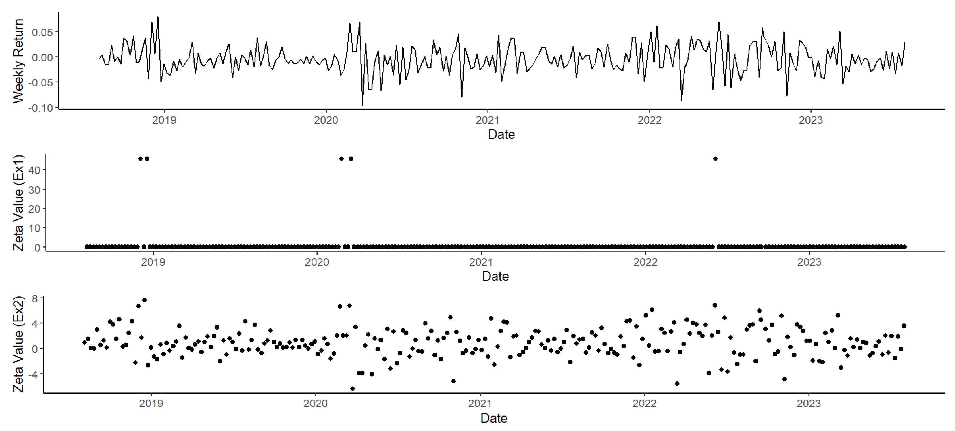
It is worth noting that the random variables in Table 3 always take positive values, so the first example in this application would fit the original optimisation framework proposed by Dhaene et al. [1]. The positiveness of ${\zeta }_i$ in Example 1 for this application can be deduced from Remark 3. For example, let us select the NASDAQ fund ($i=2$), which was the riskiest investment fund. The sample values of the weighted random variable ${\zeta }_2$ for the two examples are shown in Figure 1. The ${\zeta }_2$ in Example 1 has $c=6.218\%$ associated, and the approximated value of $\mathbb{E}\left[X_2\right]$ is $-0.326\%$, so $c-\mathbb{E}\left[X_2\right]=6.544\%>0$. Recalling that $Y_2=\mathbb{1}\left[X_2\le 6.218\%\right]$, now, we have to determine the sign of $\mathbb{E}\left[X_2{Y}_2\right]-\mathbb{E}\left[X_2\right]\mathbb{E}\left[Y_2\right]$. The sign of the sample value of this expression is negative, $-0.462\%+0.326\%0.98084$. According to Table 1, ${\zeta }_2$ is negative only when $\mathbb{1}\left[X_2\le 6.218\%\right]\ge \left(6.218\%0.98084+0.462\%\right)/\left(6.218\%+0.326\%\right)=1.00258$. However, this is not feasible since $Y_2$ takes only two values (0 or 1), and both are smaller than $1.00258$. The same reasoning can be followed by the rest of the funds in Example 1. Figure 1 shows that sample values of ${\zeta }_2$ for Example 1 take only positive values. By contrast, the random variables in Table 4 may take positive and negative values, as shown in Figure 1 for the sample values of ${\zeta }_2$ of Example 2. Therefore, the second example in this application would fit the generalised optimisation framework (1), but not the original setting (see Remark (6)).

6. Conclusions

In this paper, we generalised the capital allocation framework proposed by Dhaene et al. [1]. We proved that the haircut capital allocation principle can now be accommodated by that general optimisation framework. Under this general capital allocation setting, we provide an alternative and interpretable form to obtain the optimal solution to the quadratic optimisation problem that complements the existing geometrical proof. All required steps to obtain the optimal solution to that capital allocation framework were described in order to be easy to follow by a broad (not necessarily expert) audience. We argue that the majority of relevant scenarios from a risk management perspective can be represented in our capital allocation framework.

The theoretical findings were complemented with a financial illustration to evaluate the market risk for a set of investment funds. We showed how the haircut capital allocation principle can be applied in a real context to analyse the risk of each investment fund and to rank them based on their relative riskiness. The two examples of weighted random variables proposed in the study to define the haircut capital allocation principle as a quadratic optimisation problem were estimated in the illustration. We showed that the weighting random variable involved in the first example only took positive values in the illustration and, therefore, would fit the optimisation setting of Dhaene et al. [1]. By contrast, the weighted random variable involved in the second example took positive and negative values in the illustration and, therefore, would fit the generalised optimisation framework proposed in this study, but not the optimisation setting of Dhaene et al. [1].

To conclude, capital allocation principles defined as the outcomes of optimisation problems contribute to a deeper understanding of the implications and limitations of using a particular capital allocation principle. Providing a unified optimisation setting of capital allocation principles is useful for risk managers to select the most-adequate allocation principle in a specific risk context. The availability of a unified optimisation framework eases the risk management’s task of comparison between capital allocation principles. The generalised optimisation framework defined in our study includes the widely used haircut capital allocation principle in the unified optimisation setting. It, therefore, represents an improvement from a risk management point of view. However, our study is not without limitations. The analysis was carried out considering the quadratic optimisation criterion in a hierarchical corporate structure with one organisational level. A natural extension of our study is to consider other optimisation criteria, such as the absolute deviation criterion and hierarchical corporate structures with two or more organisational levels. Another potential future line of research is to consider the haircut capital allocation principle in portfolios with nonlinear risk aggregation.

References

1. Dhaene, J.; Tsanakas, A.; Valdez, E.A.; Vanduffel, S. Optimal Capital Allocation Principles. J. Risk Insur. 2012, 79, 1–28. [Google Scholar] [CrossRef]
2. Cao, W.; Duan, X.; Niu, X. Access to finance, bureaucracy, and capital allocation efficiency. J. Econ. Bus. 2023, 106125. [Google Scholar] [CrossRef]
3. Kempf, E.; Luo, M.; Schäfer, L.; Tsoutsoura, M. Political ideology and international capital allocation. J. Financ. Econ. 2023, 148, 150–173. [Google Scholar] [CrossRef]
4. Batrancea, L.M. An Econometric Approach on Performance, Assets, and Liabilities in a Sample of Banks from Europe, Israel, United States of America, and Canada. Mathematics 2021, 9, 3178. [Google Scholar] [CrossRef]
5. Li, Q.; Sun, H.; Tao, Y.; Ye, Y.; Zhan, K. The fault-tolerant and error-correction mechanism and capital allocation efficiency of state-owned Enterprises in China. Pac.-Basin Financ. J. 2023, 80, 102075. [Google Scholar] [CrossRef]
6. Chi, Y.L. Owners’ portfolio diversification and internal capital allocation. Pac.-Basin Financ. J. 2022, 71, 101676. [Google Scholar] [CrossRef]
7. Dhaene, J.; Goovaerts, M.; Kaas, R. Economic Capital Allocation Derived from Risk Measures. N. Am. Actuar. J. 2003, 7, 44–56. [Google Scholar] [CrossRef]
8. Belles-Sampera, J.; Guillen, M.; Santolino, M. Risk Quantification and Allocation Methods for Practitioners; Amsterdam University Press: Amsterdam, The Netherlands, 2017. [Google Scholar]
9. McNeil, A.J.; Frey, R.U.; Embrechts, P. Quantitative Risk Management: Concepts, Techniques and Tools; Princeton University Press: Princeton, NJ, USA, 2015. [Google Scholar]
10. Gaillardetz, P.; Mireku, E.O. Worst-Case Valuation of Equity-Linked Products Using Risk-Minimizing Strategies. N. Am. Actuar. J. 2022, 26, 64–81. [Google Scholar] [CrossRef]
11. Belles-Sampera, J.; Guillen, M.; Santolino, M. Compositional methods applied to capital allocation problems. J. Risk 2016, 19, 15–30. [Google Scholar] [CrossRef]
12. Kalkbrener, M. An axiomatic approach to capital allocation. Math. Financ. 2005, 15, 425–437. [Google Scholar] [CrossRef]
13. Upretee, S.; Brazauskas, V. Computing and Estimating Distortion Risk Measures: How to Handle Analytically Intractable Cases? N. Am. Actuar. J. 2022, 0, 1–21. [Google Scholar] [CrossRef]
14. Tasche, D. Risk Contributions and Performance Measurement; Working Paper; Zentrum Mathematik SCA: Munich, Germany, 2000. [Google Scholar]
15. Buch, A.; Dorfleitner, G.; Wimmer, M. Risk capital allocation for RORAC optimization. J. Bank. Financ. 2011, 35, 3001–3009. [Google Scholar] [CrossRef]
16. Kang, W.Y.; Poshakwale, S. A new approach to optimal capital allocation for RORAC maximization in banks. J. Bank. Financ. 2019, 106, 153–165. [Google Scholar] [CrossRef]
17. Urbina, J.; Santolino, M.; Guillen, M. Covariance Principle for Capital Allocation: A Time-Varying Approach. Mathematics 2021, 9, 2005. [Google Scholar] [CrossRef]
18. Costa, G.; Kwon, R. Generalized risk parity portfolio optimization: An ADMM approach. J. Glob. Optim. 2020, 78, 207–238. [Google Scholar] [CrossRef]
19. Asimit, V.; Peng, L.; Wang, R.; Yu, A. An efficient approach to quantile capital allocation and sensitivity analysis. Math. Financ. 2019, 29, 1131–1156. [Google Scholar] [CrossRef]
20. Myers, S.C.; Read, J.A. Capital Allocation for Insurance Companies. J. Risk Insur. 2001, 68, 545–580. [Google Scholar] [CrossRef]
21. Durán-Santomil, P.; Otero-González, L. Capital Allocation Methods under Solvency II: A Comparative Analysis. Mathematics 2022, 10, 303. [Google Scholar] [CrossRef]
22. Baione, F.; De Angelis, P.; Granito, I. Capital allocation and RORAC optimization under solvency 2 standard formula. Ann. Oper. Res. 2021, 299, 747–763. [Google Scholar] [CrossRef]
23. Furman, E.; Kye, Y.; Su, J. A Reconciliation of the Top-Down and Bottom-Up Approaches to Risk Capital Allocations: Proportional Allocations Revisited. N. Am. Actuar. J. 2021, 25, 395–416. [Google Scholar] [CrossRef]
24. Belles-Sampera, J.; Guillen, M.; Santolino, M. GlueVaR risk measures in capital allocation applications. Insur. Math. Econ. 2014, 58, 132–137. [Google Scholar] [CrossRef]
25. Xu, M.; Hu, T. Stochastic comparisons of capital allocations with applications. Insur. Math. Econ. 2012, 50, 293–298. [Google Scholar] [CrossRef]
26. Balog, D.; Bátyi, T.L.; Csóka, P.; Pintér, M. Properties and comparison of risk capital allocation methods. Eur. J. Oper. Res. 2017, 259, 614–625. [Google Scholar] [CrossRef]
27. Urbina, J.; Guillen, M. An application of capital allocation principles to operational risk and the cost of fraud. Expert Syst. Appl. 2014, 41, 7023–7031. [Google Scholar] [CrossRef]
28. Canna, G.; Centrone, F.; Rosazza Gianin, E. Haezendonck-Goovaerts capital allocation rules. Insur. Math. Econ. 2021, 101, 173–185. [Google Scholar] [CrossRef]
29. Targino, R.S.; Peters, G.W.; Shevchenko, P.V. Sequential Monte Carlo Samplers for capital allocation under copula-dependent risk models. Insur. Math. Econ. 2015, 61, 206–226. [Google Scholar] [CrossRef]
30. Bauer, D.; Kamiya, S.; Ping, X.; Zanjani, G. Dynamic capital allocation with irreversible investments. Insur. Math. Econ. 2019, 85, 138–152. [Google Scholar] [CrossRef]
31. Boonen, T.J. Static and dynamic risk capital allocations with the Euler rule. J. Risk 2019, 22, 1–15. [Google Scholar] [CrossRef]
32. Boonen, T.J.; Guillen, M.; Santolino, M. Forecasting compositional risk allocations. Insur. Math. Econ. 2019, 84, 79–86. [Google Scholar] [CrossRef]
33. Tsanakas, A. Dynamic capital allocation with distortion risk measures. Insur. Math. Econ. 2004, 35, 223–243. [Google Scholar] [CrossRef]
34. Zaks, Y.; Tsanakas, A. Optimal capital allocation in a hierarchical corporate structure. Insur. Math. Econ. 2014, 56, 48–55. [Google Scholar] [CrossRef]
35. Cai, J.; Wang, Y. Optimal capital allocation principles considering capital shortfall and surplus risks in a hierarchical corporate structure. Insur. Math. Econ. 2021, 100, 329–349. [Google Scholar] [CrossRef]
36. Boonen, T.J.; Tsanakas, A.; Wüthrich, M.V. Capital allocation for portfolios with nonlinear risk aggregation. Insur. Math. Econ. 2017, 72, 95–106. [Google Scholar] [CrossRef]
37. Denault, M. Coherent allocation of risk capital. J. Risk 2001, 4, 1–34. [Google Scholar] [CrossRef]
38. Boonen, T.J. τ-value for risk capital allocation problems. Oper. Res. Lett. 2020, 48, 752–757. [Google Scholar] [CrossRef]
39. Hougaard, J.L.; Smilgins, A. Risk capital allocation with autonomous subunits: The Lorenz set. Insur. Math. Econ. 2016, 67, 151–157. [Google Scholar] [CrossRef]
40. Grechuk, B. Extended gradient of convex function and capital allocation. Eur. J. Oper. Res. 2023, 305, 429–437. [Google Scholar] [CrossRef]
41. Tsanakas, A.; Barnett, C. Risk capital allocation and cooperative pricing of insurance liabilities. Insur. Math. Econ. 2003, 33, 239–254. [Google Scholar] [CrossRef]
42. Tsanakas, A. To split or not to split: Capital allocation with convex risk measures. Insur. Math. Econ. 2009, 44, 268–277. [Google Scholar] [CrossRef]
43. Furman, E.; Zitikis, R. Weighted risk capital allocations. Insur. Math. Econ. 2008, 43, 263–269. [Google Scholar] [CrossRef]
44. Zaks, Y.; Frostig, E.; Levikson, B. Optimal pricing of a heterogeneous portfolio for a given risk level. ASTIN Bull. 2006, 36, 161–185. [Google Scholar] [CrossRef]
45. Van Gulick, G.; De Waegenaere, A.; Norde, H. Excess based allocation of risk capital. Insur. Math. Econ. 2012, 50, 26–42. [Google Scholar] [CrossRef]
46. Xu, M.; Mao, T. Optimal capital allocation based on the Tail Mean-Variance model. Insur. Math. Econ. 2013, 53, 533–543. [Google Scholar] [CrossRef]
47. Wang, W.; Xu, H.; Ma, T. Optimal scenario-dependent multivariate shortfall risk measure and its application in risk capital allocation. Eur. J. Oper. Res. 2023, 306, 322–347. [Google Scholar] [CrossRef]
48. Magnus, J.; Neudecker, H. Matrix Differential Calculus with Applications in Statistics and Econometrics; Wiley Series in Probability and Statistics; Wiley: Hoboken, NJ, USA, 2019. [Google Scholar]
49. R Core Team. R: A Language and Environment for Statistical Computing; R Foundation for Statistical Computing: Vienna, Austria, 2023. [Google Scholar]
50. Gurrola-Perez, P.; Murphy, D. Filtered Historical Simulation Value-at-Risk Models and Their Competitors; Bank of England Working Paper; Bank of England: London, UK, 2015; pp. 1–30. [Google Scholar] [CrossRef]
51. Hendricks, D. Evaluation of Value-at-Risk Models Using Historical Data. Econ. Policy Rev. 1996, 2, 39–70. [Google Scholar] [CrossRef]
52. Linsmeier, T.J.; Pearson, N.D. Value at Risk. Financ. Anal. J. 2000, 56, 47–67. [Google Scholar] [CrossRef]
53. Denuit, M.; Dhaene, J.; Goovaerts, M.; Kaas, R. Actuarial Theory for Dependent Risks. Measures, Orders and Models; John Wiley & Sons Ltd.: Chichester, UK, 2005. [Google Scholar]
Figure 1. Weekly returns of the NASDAQ index for the period under study, followed by the sample values of the two weighted random variables ζ 2 reported in Table 3 and Table 4, respectively. The ζ 2 weighted random variable derived from Example 1 is always positive in this application.
Mathematics 11 03846 g001