Abstract
The stock index is actively used for the realization of profits using derivatives and via the hedging of assets; hence, the prediction of the index is important for market participants. As market uncertainty has increased during the COVID-19 pandemic and with the rapid development of data engineering, a situation has arisen wherein extensive amounts of information must be processed at finer time intervals. Addressing the prevalent issues of difficulty in handling multivariate high-frequency time-series data owing to multicollinearity, resource problems in computing hardware, and the gradient vanishing problem due to the layer stacking in recurrent neural network (RNN) series, a novel algorithm is developed in this study. For financial market index prediction with these highly complex data, the algorithm combines ResNet and a variable-wise attention mechanism. To verify the superior performance of the proposed model, RNN, long short-term memory, and ResNet18 models were designed and compared with and without the attention mechanism. As per the results, the proposed model demonstrated a suitable synergistic effect with the time-series data and excellent classification performance, in addition to overcoming the data structure constraints that the other models exhibit. Having successfully presented multivariate high-frequency time-series data analysis, this study enables effective investment decision making based on the market signals.
Keywords:
multivariate high-frequency time-series data; deep learning; ResNet; attention mechanism; stock index; S&P 500; KOSPI; DJIA MSC:
68T07
1. Introduction
According to the semi-strong form of the efficient market hypothesis (EMH), which posits that both historical and currently available public information are reflected in prices, it is argued that deriving excess profits is unattainable through the technical analysis of past stock prices or the fundamental analysis of company disclosures [1]. Nevertheless, there exists an anomalous phenomenon where firms with low price-to-book ratios (PBR) (value stocks) consistently record higher returns compared to firms with high PBR (growth stocks) [2]. Even Fama himself, a proponent of the EMH, asserts through empirical research on PBR that it offers explanatory power for the systematic risk of individual firms [3,4]. The constraints imposed by bounded rationality can limit arbitrage and instances of overreaction and underreaction to market shocks, as well as empirical analyses of specific investment strategies, providingnumerous counterexamples from the perspective of behavioral economics [5,6,7]. Through such empirical analyses, the significance of the EMH and random walk behavior has considerably diminished. Conversely, in the case of technical analysis that studies the market itself, much research that analyzes stock prices using time-series analysis as the main methodology was actively conducted.
Time-series analysis is used in various domains to investigate the influence of the past on the future. In particular, time-series analysis has been studied for a long time in the finance and economic sectors, where predictions for the future are directly related to monetary values. Ref. [8] proposed an autoregressive conditional heteroskedasticity (ARCH) model that simulates volatility using past observations. Ref. [9] standardized the ARCH model as a generalized autoregressive conditional heteroskedasticity (GARCH) model, allowing for a much more flexible lag structure. However, as ARCH and GARCH are focused on daily volatility, applying them to high-frequency data, which have been dominantly used recently owing to big data technology, is difficult. Therefore, a functional data analysis method that assumes the data observed over time as a continuous curve is widely used in combination with time-series models. Ref. [10] proposed a functional version of the ARCH for high-resolution tick data. The authors addressed the importance of balancing generality and mathematical feasibility when constructing the model. Ref. [11] suggested a functional GARCH model in which the current observation’s conditional volatility function is provided as a functional linear combination of the paths of both the past squared observation and its volatility function. Ref. [12] provided time-series prediction by utilizing functional partial least square regression with GARCH. This study highlights the challenges posed by high-dimensional and high-frequency financial data. Ref. [13] analyzed the movement of the Indonesian stock exchange (IHSG) by the GARCH model with the market indices and the macroeconomic variables. The authors figured the positive or negative effects of variables and derived the major features among the variables, which have a significant effect on the IHSG.
The deep learning technology has been leveraged worldwide. Certain major contributions to this are based on LeCun’s work on solving the training time problem of a model using a backpropagation algorithm [14]. In addition, a restricted Boltzmann machine was proposed to prevent overfitting [15]. Furthermore, the application of the activation function solved the problem of linear transformation effectively. As the relevant studies based on these foundations have rapidly gained momentum, with the evolution of deep learning methodologies [16], the research on capital market prediction is also being conducted more actively.
Ref. [17] proposed a model that mixed the probabilistic neural network (NN) model and C4.5 decision tree to predict the direction of the Taiwan stock index. Ref. [18] predicted the fluctuation of stock returns via the ensemble method of a homogeneous NN. Ref. [19] proposed a model predicting the direction and index value of S&P 500 with S&P 500 and 27 financial variables using an artificial NN. Refs. [20,21] conducted studies that approached the stock index through wavelet transformation. Ref. [20] combined an autoencoder with long short-term memory (LSTM). The proposed framework introduces the method for extracting deep invariant daily features of financial time-series. Furthermore, Ref. [21] used an artificial NN and a convolutional neural network (CNN); addressing a CNN predicts the financial time-series better than the other considered architectures in the research. The author emphasized that feature preprocessing is one of the most crucial parts in stock price forecasting. Ref. [22] proposed a model combining a genetic algorithm and CNN that exhibited effective performance in predicting fluctuations in the KOSPI using the KOSPI and technology indices. The author also demonstrated that CNN have shown promise in handling time-series data due to their ability to extract local features.
Ref. [23] suggested a model to predict the direction of daily fluctuations of S&P’s depositary receipts exchanged traded fund trust (ticker symbol SPY) using past SPY data and 60 financial variables through principal component analysis using artificial NN. This study notes that the preprocessing step is critical in improving the performance of the techniques and achieving reasonable accuracy. Ref. [24] analyzed the profitability of stock portfolios using LSTM. Ref. [25] proposed an algorithm for inputting stock index variables into LSTM via complete ensemble empirical mode decomposition with adaptive noise. A study was conducted to predict the price of SPY after 5 min using a model that combined LSTM with CNN [26]. Ref. [27] suggested a hybrid model based on LSTM and variational mode decomposition for stock price prediction. To predict US and Taiwan stocks, a graph-based CNN-LSTM model was proposed [28]. In multivariate time-series stock price data, which consisted of daily price data of five stock markets, a dynamic conditional correlation GARCH with an artificial NN was proposed by [29] for predicting risk volatility. In addition, in the case of multivariate time-series analysis, [30] proposed an encoder–decoder-based deep learning algorithm to discover interdependencies between timeseries. Recently, a univariate time-series forecasting model, neural basis expansion analysis for interpretable time-series forecasting (N-BEATS), was proposed [31]. N-BEATS showed a powerful performance using ensemble methods with the various error terms and residual stacking algorithm with the time-series trend and seasonality.
Among the various developments, the evolution of deep-learning-based transformers is noteworthy [32]. The transformer represents a significant advance in the field of natural language processing and opens up new possibilities for attention-based models. Scaled dot-product attention, the core algorithm of the transformer for analyzing data with time-series characteristics, was actively applied in various studies in combination with other backbone networks, such as the SE-NET of image classification [33] and BERT of natural language processing [34]. Ref. [35] presented a prediction model combining wavelet transform and the attention mechanism with a recurrent neural network (RNN) and LSTM as the backbone network based on the daily open, high, low, close, and adjusted close price and trading volume data of the index.
Univariate high-frequency time-series data analysis is extensively performed through functional GARCH and ARCH, and multivariate high-frequency time-series data analysis is actively studied using deep learning models. Although many advantages are realized by analyzing high-frequency data, handling multivariate high-frequency time-series data is extremely difficult owing to the multicollinearity problem of mathematical models [36]. An analysis using numeric data primarily uses deep learning methodologies based on RNNs. The RNN family processes time-series data by continuously inputting data from the beginning to the end through the hidden state for model learning [37]. In this process, structural constraints are required for model learning. In addition, in the RNN-based algorithm, as the features of the data used for learning increase, the amount of information that needs to be stored in a hidden state increases; thus, resource problems are frequently caused in computing hardware [38]. Moreover, the performance tends to improve as the layers of a deep learning model deepen; however, in an RNN series, the problem of gradient vanishing due to layer stacking is common [39]. To overcome these issues, this study proposes a novel algorithm that combines the following two algorithms for handling multivariate high-frequency time-series data. ResNet enables the characteristics of the initial input features to be efficiently transmitted to the output layer by the residual block, despite the stacking of the complex CNN [40]. The attention mechanism reinforces the main features between the input data according to the context of the data [32] and exhibits suitable synergistic effect, particularly in sequence data [34]. Consequently, the context could be appropriately reflected from the hidden patterns and time-series characteristics of the data to the prediction performance.
In summary, our major contributions are as follows:
- The theme of our research is highly unprecedented in the financial field to the best of our knowledge. With three market index datasets with micro time interval time-series data, we validated our proposed end-to-end model for multivariate high-frequency data. Especially in the case of S&P 500, it exploits the whole 500 tickers’ hourly data as an input variable in the models.
- We illustrated our data pipeline procedures for the proposed model in detail. This enables the model to train from batches of randomly shuffled samples. This approach positively affects the robustness of the model by updating the weights of the model from the entire period of the time-series during model training.
- The proposed model is a hybrid model that combines two state-of-the-art models, each of which has proven its performance in academic consensus. The algorithmic approach that enhances data features based on time-series context, alongside the algorithm focusing on extracting variable feature patterns, has facilitated performance enhancement in terms of accuracy, while concurrently reducing both model training duration and inference time.
The remainder of this paper is organized as follows: In Section 2, we describe the datasets, the data preprocessing, the attention mechanism, three types of deep learning models, metrics for performance comparison, and a clear depiction of the research scheme. In Section 3, we illustrate the superiority of our proposed method in terms of performance compared with the RNN and LSTM methods, with and without the attention mechanism, and ResNet without attention. We discuss our findings in Section 4 and provide the conclusion in Section 5.
2. Materials and Methods
2.1. Dataset
The primary interest of this study is the prediction of the rise and fall of the capital market index representing the stock market using multivariate high-frequency time-series data. The S&P 500, KOSPI, and Dow Jones Industrial Average (DJIA) were the key indices selected. Using the collected data, the daily fluctuation information was labeled based on the closing price of the day compared with the previous day of each index. The graphs and statistics for each index as the target variable are presented in Figure 1 and Table 1, respectively.
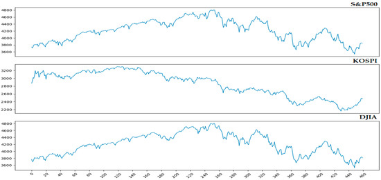
Figure 1.
Graph of fluctuations in the selected indices.The y-axis indicates the value of the index, and the x-axis denotes the trading day of each index.

Table 1.
Summary statistics of the target indices, including the time points, mean, standard deviation, maximum, minimum, and quartile of the three market indices.
The S&P 500 is a stock index that represents the US stock market and is a market capitalization-based market index that incorporates individual stocks traded in the market according to their market price ratio, based on 500 large companies listed in the US stock market. The KOSPI is an index indicating the quantitative difference between the Korean KOSPI-listed stock market at the time of comparison and the reference time, which is the market capitalization as of 4 January 1980. DJIA is a stock market index that monitors the performance of thirty large, publicly traded companies in the United States. The index’s value is derived from the weighted average of the stock prices of these thirty companies. To predict the daily index fluctuation information of each index, we collected time-series data related to each index. The detailed specifications for each dataset are as follows:
2.1.1. S&P 500
The data were collected from the beginning of 2021 to 31 October 2022 via the Yahoo Finance API Python library yfinance. The list of variables refers to the ‘List of S&P 500 companies’ Wikipedia page, recorded as of December 2022. The dataset consists of the S&P 500 index and 500 tickers, three of which—Alphabet, Fox Corporation, and News Corp—are divided into two classes. Thus, daily 1-h interval adjusted-close-price time-series values of 504 variables were collected. As a window size of 10, a total of 10 days of time-series data were configured to be used to predict daily price fluctuations. In other words, one sample of the data used to predict the rise and fall of the one-day index is the massive-multivariate high-frequency data with 35,280 features: 504 (variables) × 7 (intro-day time points) × 10 (window size). For deep learning, the data structure must be identical throughout. In the original data collected, the stock market closed early on November 26, 2021; therefore, the time points insufficient for that dimension were equally padded with the closing price (504 variables × 3 missing time points). In addition, in the case of a missing value, the previous price is incorporated, and if a missing value still persists thereafter, the price immediately after is substituted therein.
2.1.2. KOSPI
From 4 January 2021 to 15 November 2022, considering the trading days of the Korea Stock Exchange, the directions in the closing index on the day relative to the previous day’s closing index of the KOSPI were collected as target data. To predict the target data, 13 variables that feature closing prices at 5-min intervals were collected as input variables corresponding to the target variable period. The input variables were selected after careful consideration based on previous studies. The input variables consist of the KOSPI, Kodex 10-Year Korea Treasury Bond (KTB) Futures [41,42], Kodex United States Dollar Futures [43,44], and the top 10 KOSPI stocks based on market capitalization [45]. The window size is 5, which is configured to use a total of five days of time-series data to predict daily price fluctuations. In other words, one sample of the data used to predict the rise and fall of the daily index is multivariate high-frequency with 5070 features: 13 (variables) × 78 (intro-day time points) × 5 (window size). In the case of KOSPI, the exchange opens 1 h later on the first day of the New Year, and therefore, we increased the dimensions by 12 through data preprocessing and padded it with the price immediately after (13 variables × 12 missing time points). The preprocessing for missing values was the same as that for the S&P 500 dataset.
2.1.3. DJIA
The data were collected from the beginning of 2021 to 31 October 2022 via the Yahoo Finance API Python library yfinance. The dataset consists of the daily 1-h interval open, high, low, and close (OHLC) price of the three major US stock market indices, including the DJIA, S&P 500, and Nasdaq Index and comprises a total of 12 variables. Compared with the two datasets described earlier, the number of daily features in this dataset was relatively small; therefore, the window size was set to 20. Hence, a total of 20 days of time-series data was configured to be used to predict fluctuations in the daily price of the DJIA. For clarity, one sample of the data used to predict the rise and fall of the one-day index is the massive-multivariate high-frequency data with 1680 features: 12 (variables) × 7 (intro-day time points) × 20 (window size). The preprocessing for missing values was 12 variables × 3 missing time points, the same as S&P 500.
2.2. Methods
2.2.1. Data Preprocessing
- Min–max Normalization
The purpose of this study is to conduct an efficient analysis of the multivariate high-frequency data and forecast the rise and fall of the corresponding stock index. To achieve this, the multivariate data pertaining to the movements of the target market index are subject to min–max scaling on a variable-wise basis, with values scaled between 0 and 1 in accordance with the training set. The calculation for variable-wise min–max scaling based on the training set is as follows:
- 2.
- Additional Preprocessing for Proposed Model
Each vector in X is sampled by the window size = w, expanding the dimension by the number of days included. Hence, the sample of the tth window training dataset has the following data structure.
where i = 1, 2, …, mth variable, for j = 1, 2, …, wth day, and = [[], [], …, []].
Figure 2 depicts the data preprocessing procedure for the proposed model. First, the price information for each timestamp is min–max scaled to values between 0 and 1. (To facilitate comprehension, in Figure 2, values that are close to 1 are represented as white, whereas values that are close to 0 are represented as black.) This information is then divided into window units and arranged in rows by date, resulting in a two-dimensional vector that shares the same time zone as a column. This process is repeated for each variable, creating channelized multivariate time-series data.
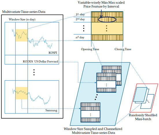
Figure 2.
Preprocessing of the multivariate high-frequency time-series data for ResNet.
Finally, randomly shuffled mini-batches are generated from the data for use in the proposed model training. Figure 3 illustrates the process of constructing two randomly shuffled mini-batches using the S&P 500 as an example.
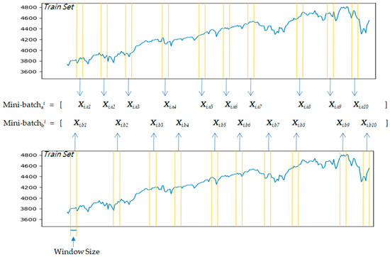
Figure 3.
Example of two randomly shuffled mini-batches with S&P 500 time-series data.
Overall, the proposed model aims to recognize each preprocessed data sample as an independent image, with no dependence on the sequential relationship between samples. Thus, the data pipeline for the model was devised to randomly shuffle the samples, enabling the model to be trained based solely on continuity within the window-sized sample.
2.2.2. Attention Mechanism
The attention mechanism is based on the concept of focusing only on the input data related to the value to be predicted rather than referring to the entire input data. Several types of attention mechanisms exist, including Bahdanau attention [46] and Luong attention [47]. In this study, scaled dot-product attention (SDA), introduced in the transformer algorithm, which exhibited excellent performance in text analysis, was used [32]. In addition to the SDA, the position-wise feed forward networks (PFFN) and layer normalization (LN) [48] described in the transformer were used. In particular, LN corrects the discrepancy between the features of the raw data in the process of finding the optimal solution as learning progresses.
As one sample of the input data at the tth time window with is denoted as , SDA consists of random coefficients vectors with queries as , keys as , and values as , where , , and have the same dimensions as . The initial values of , , and were set at random and tuned to satisfactory values that considered contextual information during the model training. With the dot product of , , and ,vectors, , , and are calculated, respectively. SDA is defined as follows:
Eventually, the samples were changed to the values mapped using the SDA function. After the SDA process, the modified data were input into the PFFN, which is defined as follows:
This function is applied to each position separately and identically; using g(z) in between, which is a ReLU function, it increases the effectiveness of backpropagation [16]. Referring to the study conducted by [32], the dimensions of the input and output were set to , and the dimensions of the inner layer were set to twice those of . Finally, the data passed SDA, and the PFFN was subjected to LN adjustment, which was calculated as follows:
The aforementioned attention mechanism assumes that X is a single variable; however, because it was used in multivariate data, it was applied variably. Figure 4 depicts the algorithm of the variable-wise SDA of X in the tth window. Consequently, the variable input to the variable-wise SDA is mapped to , and the manner in which is input to the model changes according to the backbone network.
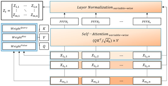
Figure 4.
Variable-wise scaled dot-product attention module.
2.2.3. ResNet18
ResNet [40] was the 2015 winner of the ImageNet Large Scale Visual Recognition Challenge, a prominent image classification contest. This model was evaluated to perform better than human image recognition, as its image classification error rate was only 3.6%. It is designed to solve the degradation of the training accuracy problem of deep networks by using the deep residual learning framework, which causes layers to fit a residual mapping H(z). This study enables a stacked nonlinear function, denoted as F(z), to fit H(z) − z, assuming that multiple nonlinear layers can asymptotically approximate a complicated function and also that H(z) − z can be approximated asymptotically to F(z) [40]. Consequently, the original function F(z) becomes F(z) + z for H(z), and H(z) is implemented by the residual block consisting of convolutional operations [49] and through identity mapping by shortcut connections [40]. A residual block with two convolutional layers is expressed as follows:
ResNet18 consists of one general convolutional layer, eight residual blocks with two convolutional layers, and one fully connected dense layer. Because the ResNet model was conceived for classifying 1000 types of images, the original input shape of ResNet has three channels for color images, and the output layer is designed to pass the Softmax activation function. In this study, for modeling, the three channels of ResNet18 were expanded to a variable number of channels, and the Softmax function was substituted with the sigmoid function for binary classification. Figure 5 shows the depiction and residual block algorithm, where sample is input into ResNet.
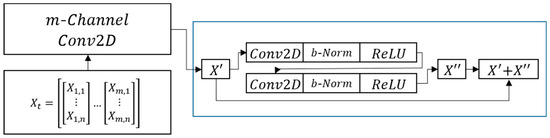
Figure 5.
Process of inputting X in the tth window to ResNet, and the structure of the residual block. Conv2D means a two dimensional convolutional neural network, and b-Norm is batch normalization.
2.2.4. RNN
An RNN is a deep learning model that processes inputs and outputs as a sequence unit of a window size [37]. In the case of vanilla deep NN, which are stacked in general layers, the performance of sequential data analysis is inferior because historical information cannot be reflected in the learning process. To overcome this issue, an RNN was designed with a structure comprising hidden layers and an output layer. This functions through a memory cell that sends a result through an activation function and a hidden state, which is the value sent to the next time point. In short, the memory cell at time t uses the hidden state sent by the memory cell at time t − 1 as the input to calculate the hidden state at time t for the next layer. Let the hidden state at time t be denoted as vector ht, which is calculated as follows:
Each output layer is another path of the memory cell, and one of its output values at time t, denoted by yt, is calculated as follows:
Figure 6 shows the RNN used in this study, and a feed forward neural network (FFNN) for binary classification was constructed in the output layer according to the dimension of the variables.
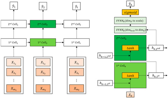
Figure 6.
Recurrent neural network (RNN) for multivariate time-series data. Left side of the figure illustrates the typical construct of the RNN-family model, and the right side demonstrates multivariate two-layer RNN with feed forward neural networks (FFNNs) for X at the kth window.
2.2.5. LSTM
In RNN, the longer the period of sequential data, the less sufficient is the previous information transmitted to the output layer, and it has the limitation of exhibiting the effect only for relatively short sequences [39]. As an alternative, the LSTM algorithm, which adds forget, input, and output gates to the memory cells of the hidden layer, was proposed [50]. The memory cell at time t + 1 receives the cell state at time t denoted as Ct, which is calculated as follows:
where is the forget gate at time t, which is calculated by
is the input gate at time t, and is another input gate at time t, which is calculated as follows:
Consequently, the output gate at time t, denoted as , enables the calculation of the hidden state at time t denoted as and transfers it to the output layer and memory cell at time t + 1. Finally, is calculated as follows:
Figure 7 illustrates the LSTM used in this study, and FFNNs for binary classification were considered in the output layer for the dimension of the variables.
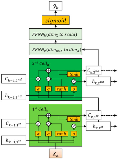
Figure 7.
Multivariate two-layer LSTM with FFNNs for X at the kth window.
2.3. Metrics of Performance: F1-Score
To calibrate the imbalances among the training, validation, and test datasets using metrics, we used the F1-score as the main metric to measure the model performance. Precision and recall are the two most representative metrics used when the data are imbalanced and are the basis of the F1-score. Let TP be the number of true positives, TN the number of true negatives, FP the number of false positives, and FN the number of false negatives; accordingly, the precision and recall are calculated, respectively, as follows:
Precision is an index evaluated from the perspective of prediction by penalizing type-I errors, and recall is an index evaluated from the perspective of actual values by penalizing type-II errors. Precision and recall exhibit a trade-off relationship, and the F1-score evaluates the performance of the model with the harmonic mean of these two measures and is calculated as follows:
The F1-score was calibrated to be more affected by the smaller value of precision and recall using the harmonic average.
2.4. Research Design
The process of deriving a classification model using a deep learning approach can be outlined as follows: 1. data collection and preprocessing, which is the initial step, involves gathering and preprocessing the data; 2. train/validation/test set partitioning and normalization; 3. feature engineering, which is the technique applied to enhance the representation of the data; 4. model generation, which involves the architectures and the layer design; 5. model training using the train set and determining optimal train parameters with the validation set; 6. model performance evaluation using the test dataset; and 7. derivation of the optimal model through model comparison. Our study follows this general deep learning approach.
For clarity, we demonstrate the depiction of the entire study design. Based on the above methodologies, an algorithm for predicting the indices of daily fluctuations was designed.
Figure 8 shows the overall configuration and flow of the algorithm in detail. Our research procedure is divided into two parts: One is the preprocessing part for data input, and the other is the depiction of the transmission of data input according to the deep learning model to be used.
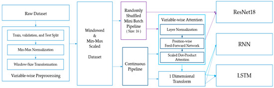
Figure 8.
Scheme of the study depicting how the raw data are preprocessed and fed into the models as input features.
In the case of the datasets, 75% training data were used for model training, and 25% test data were used for model comparison. The last 25% of the training set was used as the validation set to determine the best epoch for training the models. Min–max normalization was performed based on the training set. Several studies have presented the importance of data normalization to improve data quality and the performance of machine learning algorithms [51]. For modeling, the window size was configured as 10 days for S&P 500, 5 days for KOSPI, and 20 days for the DJIA. The datasets for training, validation, and testing were transformed with a sample structure corresponding to the window size of each dataset.
Depending on the final type of the deep learning method, that is, RNN, LSTM, and ResNet18, the preprocessed data are transmitted through two approaches. One approach is the continuous pipeline for the RNN and LSTM, where samples of each training set are fed into the model sequentially in the forward direction. The other approach is the data pipeline for ResNet18, which is a method for proceeding with data learning by configuring part of the data in a random manner rather than obtaining a weighted average of all the data. Consequently, the data are fed into the deep learning model in four ways, depending on whether variable-wise attention is applied through the data pipeline.
The following conditions were applied similar to those of the simulations. The aforementioned deep learning methodologies were implemented using the Colab GPU session with Python version 3.8.16, Torch 1.13.0 + cu116, Torchvision 0.14.0 + cu116, Scikit-learn 1.0.2, and Numpy 1.21.6 and were used for preprocessing and evaluation under the same Python version. The optimization algorithm for modifying the model parameters through backpropagation was RAdam [52], and its hyperparameters were as follows: learning rate = 0.001, coefficient Beta1 = 0.900, coefficient Beta2 = 0.999, and denominator eps = 1 × 10⁻⁸.
3. Results
The models were developed based on Resnet18, RNN, and LSTM to compare their performance. In particular, RNN and LSTM were designed with two layers. In addition, all the models were compared based on whether attention was applied. Thus, six models were constructed. Because the target value is 1 or 0, implying the rise or fall of the next-day index direction, respectively, the models were trained using a binary cross-entropy loss function. As the deep learning model was trained by iterating epochs, the F1-score of the validation set was measured for each epoch, and the one with the highest F1-score was determined as the optimal amount of learning. The F1-score was determined as the main metric because the label distributions of the training, validation, and test sets were different for each dataset.
3.1. S&P 500
As Table 2 illustrates, the proposed model, ResNet18 with attention, performed best among the models in terms of not only the F1-score but also all other metrics, such as the AUC, and precision of 65.07%, 57.07%, and 51.89%, respectively. The test set F1-score from ResNet exhibited enhanced performance based on application of the attention mechanism. In particular, compared with ResNet18 without attention, the proposed model increased the F1-score by 6.81%, AUC by 5.09%, and precision by 5.70%. In the case of the RNN and LSTM models, the models without the attention mechanism exhibited a gradient diminishing problem. They only output positive values, implying that the index is always expected to increase. Conversely, RNN and LSTM with attention solved the gradient reduction problem to a certain extent (almost minimally), and both AUC values slightly increased by 0.35% and 4.46%, respectively. In terms of the running time, the model based on ResNet18 dramatically reduced the time compared to RNN and LSTM. In the case of the attention incorporated models, the training speed of the ResNet model was increased by 71% and 74% compared to RNN and LSTM, respectively.
Table 2.
Results of the S&P 500 dataset by ResNet, RNN, and LSTM with or without the attention mechanism.
3.2. KOSPI
Table 3 presents the results of the experiment using the KOSPI dataset. Similar to the results of S&P 500, ResNet blended with attention exhibited a better performance than the others. Except for the F1-score of the RNN model without attention, which only predicts true values unconditionally because the gradient is lost, the proposed model performed best among the models with not only the F1-score but also in all other metrics, such as AUC, and with a precision of 68.37%, 61.64%, and 62.5%, respectively. The test set F1-score from ResNet exhibited enhanced performance upon the application of the attention mechanism. In particular, compared with ResNet18 without attention, the proposed model increased the F1-score by 13.99%, AUC by 8.28%, and precision by 11.68%. For the RNN without attention, applying attention increased AUC by 9.66%. Regarding the running time, similarly, the ResNet18-based model has reduced time compared to RNN and LSTM. In particular, in the case of the KOSPI dataset, the proposed model showed the fastest speed among all models.
Table 3.
Results for fluctuations in the KOSPI classification by ResNet, RNN, and LSTM with the Attention.
3.3. DJIA
Table 4 presents the results of the model-specific tests of the DJIA dataset. In the case of the DJIA prediction, the model we presented exhibited the best performance in all aspects of the performance indicators. The F1-score, AUC, and precision were 64.07%, 59.19%, and 62.26%, respectively. These are effects realized upon adding attention to ResNet, and the increments are 1.17%, 6.53%, and 9.56%, respectively. Neither the RNN nor the LSTM demonstrated any gradient vanishing problem on the DJIA dataset, and when the attention mechanism was incorporated, they performed 4.06% and 4.97% better on the main metric, F1-score. About running time, in the case of the attention-applied models, the ResNet model reduced the training time by 65% and 64% with respect to RNN and LSTM.
Table 4.
Results for classifying DJIA fluctuations according to the attention module between models.
4. Discussion
We conducted some research on whether the three channels typically utilized in the CNN algorithm, which are designed to input the three primary RGB colors of image data, could be effectively employed to analyze multivariate time-series data. In the course of refining the CNN algorithm, we developed an innovative method that leverages the ResNet18 model in combination with the attention mechanism to predict the direction of market index fluctuations.
As illustrated in Figure 9, using three distinct stock index datasets, we constructed a total of six models based on the three deep learning models and the inclusion or exclusion of attention. Notably, all three datasets were comprised of multivariate high-frequency data, with varying feature dimensions based on the number of variables, time points, and window size. Our experimental results demonstrated that the performance of LSTMs and RNNs is largely dependent on the data dimension. For instance, in the DJIA dataset model, which had a relatively small-dimensional feature space, both LSTM and RNN performed adequately. Moreover, when the attention module was attached, the F1-score improved for both models. However, in the case of the KOSPI dataset, which had a threefold increase in variable dimension relative to the DJIA dataset, the RNN without attention encountered a gradient diminishing problem. The findings of this research are consistent with the results of previous studies, wherein performance problems arose when dealing with a large number of features [39,53,54]. Particularly in the S&P 500 dataset, which includes massive multivariate high-frequency data, where the variable dimension is 21 times larger than that of the DJIA dataset, both LSTM and RNN without attention illustrate a gradient problem. By incorporating the attention mechanism, which emphasizes key features, the gradient loss problem was partially alleviated, and the AUC value slightly increased. Nonetheless, the performance boost from combining the attention mechanism with LSTMs and RNNs was not significantly apparent, unlike in the case of the suggested model, which yielded the best overall performance.
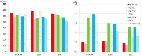
Figure 9.
Comparison of model performance based on F1-score and train time-consumption per one iteration, conducted for each dataset. s/iter: seconds per iteration; Att-Resnet: ResNet with attention; Att-RNN: RNN with attention; Att-LSTM: LSTM; and G-Diminishing: Gradient diminishing.
The superiority of the proposed algorithm can be attributed to the structural properties of the model. A key feature of the suggested model is the synergistic effect between the attention mechanism and the residual block. One of the components of the attention mechanism, the LN, is responsible for balancing the effect of feature reinforcement on the SDA context and the feature structure of the original sample [32,48]. On the other hand, the residual block, which plays a key role in ResNet, extracts minute features of variables from convolutional layers and performs the weighted average of data features passed from the previous block, which is similar to the function of the LN [40]. By combining these two functions, the model can convey the variable feature enhancement effect of the attention mechanism according to the context of the output layer, even after passing through highly complex convolutional operations.
The data pipeline also played a significant role in enhancing the performance of the proposed algorithm. Specifically, the data pipeline serves as a data transmitter that trains deep learning models using randomly shuffled mini-batches. The application of deep neural networks for predicting stock prices relies heavily on recurrent neural networks, which are known for their ability to handle time-series data effectively. However, RNN-based models require sequential input during the training phase. As a result, the latter part of the training set has a significant impact on the learning process. To address this issue, researchers have explored the use of additional techniques such as CNNs [26,28], genetic algorithms [22], and attention mechanisms [35] to improve the distribution of the initial data in time-series analysis. Nevertheless, the fundamental approach to handling time-series data remains unchanged. In this study, however, the time-series data is partitioned into samples of fixed window size, and only the information within each window is assumed to be continuous, rendering each sample as an independent unit. Therefore, mini-batch training becomes possible, as the recurrent neural network family’s hidden state, which transfers the learned information from the previous data point’s distribution, is unnecessary and unaffected by the inter-sample continuity. This approach effectively reduces the possibility of overfitting and enables the model to generalize well to unseen data [55]. Consequently, this leads to a significant reduction in the model’s training time, alleviation of memory resource requirements, and attainment of stable and high performance. Overall, the combination of the attention mechanism, residual block, and data pipeline contributed to the excellent performance of the proposed algorithm for predicting market index fluctuations using multivariate time-series data.
In the realm of univariate high-frequency time-series data analysis, mathematical operations such as functional GARCH or functional ARCH are utilized to calculate the weights of major features. However, the direct application of these methods to multivariate analysis remains challenging. Feature selection for deep learning using explainable AI, such as SHAP [56], LIME [57], and LRP [58], has been actively studied; however, it is still difficult to apply it to multivariate high-frequency time-series data. The future development of more advanced explainable AI is anticipated to address the black-box issue inherent in deep learning. Through this advancement, it is expected that services, such as models contributing to financial decision-makers through machine learning [59], could be also reliably provided via AI models. Although this study focused on predicting market index fluctuations, analyzing volatility is equally important in finance. It is anticipated that future studies will expand on this algorithm to consider volatility or intraday volatility, further enhancing its academic contributions.
5. Conclusions
This study is the benchmark of multivariate high-frequency time-series data analysis based on deep learning. We proposed a model that combines the attention mechanism with the residual block for multivariate high-frequency time-series data. Attention reinforces the ability to represent the context of the input data. ResNet18 is composed of convolutional layers that understand the features of microscopic data through feature maps. To verify the model performance, we conducted an experiment using three datasets, namely, S&P 500, KOSPI, and DJIA, and compared the model with RNN and LSTM, confirming its excellent performance in terms of several indicators, including the F1-score and the model training speed. In addition to the performance improvement, another key advantage of our model is that the algorithm requires only minimal continuity of the input sample by the size of the window, and the continuity of the input variable is not mandatory.
Though our study does not consider profitability test and simulation, intuitively, returns are dependent on an index’s directional predictive performance if it is high. Accurately predicting the direction of returns can help predict prices and increase returns as a reference for investors. As we addressed at the end of the Section 4, when conducting future research that considers direction and volatility, we would considertheoretical simulations of profitability. Consequently, the findings and concepts presented through this study will contribute to effective investment decision making by capital market stakeholders.
Author Contributions
S.K.—research idea, formulation of research goals and objectives, guidance and consulting, examination of calculation results. Y.N.—analysis of literature, analysis of experimental data, validation of model, draft and final copy of the manuscript. J.-M.K.—research idea, analysis of experimental data, literature analysis, guidance and consulting. S.H.—research idea, validation and investigating of data, writing review and editing, guidance and consulting.All authors have read and agreed to the published version of the manuscript.
Funding
This research was funded by Dong-A University, Republic of Korea (10.13039/501100002468).
Data Availability Statement
The raw dataset is available at the Yahoo Finance API. The datasets generated and/or analyzed during the current study are not publicly available due to intellectual property reasons.
Acknowledgments
The authors are thankful to the anonymous referees for their helpful comments.
Conflicts of Interest
The authors declare no conflict of interest.
Abbreviation
| X | one of the total dataset’ independent variables, such as S&P 500 with 504 variables, KOSPI with 13 variables, and DJIA with 12 variables |
| ith variable of X, where i = 1st, 2nd, …, mth variables | |
| scalar value of feature dimension, which is the number of time points in one day | |
| vector, which is the set of prices of th day of , where ∀, j = 1, 2, …, n | |
| w | size of window by the time interval, which is the size of the day |
| trainable weight vector of neural networks, where i = 1, 2, …, n | |
| trainable bias vector of neural networks, where i = 1, 2, …, n | |
| arbitrary vector |
References
- Fama, E.F. Efficient capital markets: A review of theory and empirical work. J. Financ. 1970, 25, 383–417. [Google Scholar] [CrossRef]
- Lakonishok, J.; Shleifer, A.; Vishny, R.W. Contrarian in-vestment, extrapolation, and risk. J. Financ. 1994, 49, 1541–1578. [Google Scholar] [CrossRef]
- Fama, E.F.; French, K.R. The cross-section of expected stock returns. J. Financ. 1992, 47, 427–465. [Google Scholar] [CrossRef]
- Fama, E.F.; French, K.R. Common risk factors in the returns on stocks and bonds. J. Financ. Econ. 1993, 33, 3–56. [Google Scholar] [CrossRef]
- Shiller, R.J. From efficient markets theory to behavioral finance. J. Econ. Perspect. 2003, 17, 83–104. [Google Scholar] [CrossRef]
- De Bondt, W.F.M.; Thaler, R. Does the stock market overreact? J. Financ. 1985, 40, 793–805. [Google Scholar] [CrossRef]
- Gallagher, L.A.; Taylor, M.P. Permanent and temporary components of stock prices: Evidence from assessing macroeconomic shocks. South. Econ. J. 2002, 69, 345–362. [Google Scholar]
- Engle, R.F. Autoregressive conditional heteroscedasticity with estimates of the variance of United Kingdom inflation. Econom. J. Econom. Soc. 1982, 50, 987–1007. [Google Scholar] [CrossRef]
- Bollerslev, T. Generalized autoregressive conditional heteroskedasticity. J. Econom. 1986, 31, 307–327. [Google Scholar] [CrossRef]
- Hörmann, S.; Horváth, L.; Reeder, R. A functional version of the ARCH model. Econom. Theory 2013, 29, 267–288. [Google Scholar] [CrossRef]
- Aue, A.; Horváth, L.; Pellatt, D.F. Functional generalized autoregressive conditional heteroskedasticity. J. Time Ser. Anal. 2017, 38, 3–21. [Google Scholar] [CrossRef]
- Kim, J.-M.; Jung, H. Time series forecasting using functional partial least square regression with stochastic volatility, GARCH, and exponential smoothing. J. Forecast. 2018, 37, 269–280. [Google Scholar] [CrossRef]
- Endri, E.; Abidin, Z.; Simanjuntak, T.; Nurhayati, I. Indonesian stock market volatility: GARCH model. Montenegrin J. Econ. 2020, 16, 7–17. [Google Scholar] [CrossRef]
- Boser, B.; Denker, J.S.; Henderson, D.; Howard, R.E.; Hubbard, W.; Jackel, L.D.; Laboratories, H.Y.L.B.; Zhu, Z.; Cheng, J.; Zhao, Y.; et al. Backpropagation applied to handwritten zip code recognition. Neural Comput. 1989, 1, 541–551. [Google Scholar]
- Hinton, G.E. Learning multiple layers of representation. Trends Cogn. Sci. 2007, 11, 428–434. [Google Scholar] [CrossRef] [PubMed]
- Schmidhuber, J. Deep learning in neural networks: An overview. Neural Netw. 2015, 61, 85–117. [Google Scholar] [CrossRef] [PubMed]
- Cheng, J.-H.; Chen, H.-P.; Lin, Y.-M. A hybrid forecast marketing timing model based on probabilistic neural network, rough set and C4.5. Expert Syst. Appl. 2010, 37, 1814–1820. [Google Scholar] [CrossRef]
- Tsai, C.-F.; Lin, Y.-C.; Yen, D.C.; Chen, Y.-M. Predicting stock returns by classifier ensembles. Appl. Soft Comput. 2011, 11, 2452–2459. [Google Scholar] [CrossRef]
- Niaki, S.T.A.; Hoseinzade, S. Forecasting S&P 500 index using artificial neural networks and design of experiments. J. Ind. Eng. Int. 2013, 9, 1–9. [Google Scholar]
- Bao, W.; Yue, J.; Rao, Y. A deep learning framework for financial time series using stacked autoencoders and long-short term memory. PLoS ONE 2017, 12, e0180944. [Google Scholar] [CrossRef]
- Di Persio, L.; Honchar, O. Artificial neural networks architectures for stock price prediction: Comparisons and applications. Int. J. Circuits Syst. Signal Process. 2016, 10, 403–413. [Google Scholar]
- Chung, H.; Shin, K.-S. Genetic algorithm-optimized multi-channel convolutional neural network for stock market prediction. Neural Comput. Appl. 2020, 32, 7897–7914. [Google Scholar] [CrossRef]
- Zhong, X.; Enke, D. Forecasting daily stock market return using dimensionality reduction. Expert Syst. Appl. 2017, 67, 126–139. [Google Scholar] [CrossRef]
- Fischer, T.; Krauss, C. Deep learning with long short-term memory networks for financial market predictions. Eur. J. Oper. Res. 2018, 270, 654–669. [Google Scholar] [CrossRef]
- Cao, J.; Li, Z.; Li, J. Financial time series forecasting model based on CEEMDAN and LSTM. Phys. A Stat. Mech. Its Appl. 2019, 519, 127–139. [Google Scholar] [CrossRef]
- Kim, T.; Kim, H.Y. Forecasting stock prices with a feature fusion LSTM-CNN model using different representations of the same data. PLoS ONE 2019, 14, e0212320. [Google Scholar] [CrossRef]
- Yang, Y.; Yang, Y.; Wang, Z. Research on a hybrid prediction model for stock price based on long short-term memory and variational mode decomposition. Soft Comput. 2021, 25, 13513–13531. [Google Scholar]
- Wu, J.M.-T.; Li, Z.; Herencsar, N.; Vo, B.; Lin, J.C.-W. A graph-based CNN-LSTM stock price prediction algorithm with leading indicators. Multimed. Syst. 2021, 29, 1751–1770. [Google Scholar] [CrossRef]
- Fatima, S.; Uddin, M. On the forecasting of multivariate financial time series using hybridization of DCC-GARCH model and multivariate ANNs. Neural Comput. Appl. 2022, 34, 21911–21925. [Google Scholar] [CrossRef]
- Yin, C.; Dai, Q. A deep multivariate time series multistep forecasting network. Appl. Intell. 2022, 52, 8956–8974. [Google Scholar] [CrossRef]
- Oreshkin, B.N.; Carpov, D.; Chapados, N.; Bengio, Y. N-BEATS: Neural basis expansion analysis for interpretable time series forecasting. arXiv 2019, arXiv:1905.10437. [Google Scholar]
- Vaswani, A.; Shazeer, N.; Parmar, N.; Uszkoreit, J.; Jones, L.; Gomez, A.N.; Kaiser, L.; Polosudhin, I. Attention is all you need. Adv. Neural Inf. Process. Syst. 2017, 30. [Google Scholar] [CrossRef]
- Hu, J.; Shen, L.; Sun, G. Squeeze-and-excitation networks. In Proceedings of the IEEE Conference on Computer Vision and Pattern Recognition, Salt Lake City, UT, USA, 18–22 June 2018; pp. 7132–7141. [Google Scholar]
- Devlin, J.; Chang, M.-W.; Lee, K.; Toutanova, K. Bert: Pre-training of deep bidirectional transformers for language understanding. arXiv 2018, arXiv:1810.04805. [Google Scholar]
- Qiu, J.; Wang, B.; Zhou, C. Forecasting stock prices with long-short term memory neural network based on attention mechanism. PLoS ONE 2020, 15, e0227222. [Google Scholar] [CrossRef]
- Zhang, X.; Huang, Y.; Xu, K.; Xing, L. Novel modelling strategies for high-frequency stock trading data. Financ. Innov. 2023, 9, 1–25. [Google Scholar] [CrossRef] [PubMed]
- Mikolov, T.; Karafiat, M.; Burget, L.; Honza, J.; Khudanpur, S. Recurrent neural network based language model. In Proceedings of the Interspeech, Chiba, Japan, 26–30 September 2010; pp. 1045–1048. [Google Scholar]
- Mittal, S.; Umesh, S. A survey on hardware accelerators and optimization techniques for RNNs. J. Syst. Archit. 2021, 112, 101839. [Google Scholar] [CrossRef]
- Pascanu, R.; Mikolov, T.; Bengio, Y. On the difficulty of training recurrent neural networks. In Proceedings of the International Conference on Machine Learning, PMLR, Atlanta, GA, USA, 17–19 June 2013; pp. 1310–1318. [Google Scholar]
- He, K.; Zhang, X.; Ren, S.; Sun, J. Deep residual learning for image recognition. In Proceedings of the IEEE conference on computer vision and pattern recognition, Las Vegas, NV, USA, 27–30 June 2016; pp. 770–778. [Google Scholar]
- Sharpe, W.F. Capital asset prices: A theory of market equilibrium under conditions of risk. J. Financ. 1964, 19, 425–442. [Google Scholar]
- Hwang, S.-S.; Lee, M.-W.; Lee, Y.-K. An empirical study of dynamic relationships between kospi 200 futures and ktb futures markets. J. Ind. Econ. Bus. 2020, 33, 1245–1263. [Google Scholar] [CrossRef]
- Jabbour, G.M. Prediction of future currency exchange rates from current currency futures prices: The case of GM and JY. J. Futures Mark. 1994, 44, 25. [Google Scholar] [CrossRef]
- Crain, S.J.; Lee, J.H. Intraday volatility in interest rate and foreign exchange spot and futures markets. J. Futures Mark. 1995, 15, 395. [Google Scholar]
- Kim, J.-I.; Soo, R.-K. A Study on Interrelation between Korea’s Global Company and KOSPI Index. J. CEO Manag. Stud. 2018, 21, 131–152. [Google Scholar]
- Bahdanau, D.; Cho, K.; Bengio, Y. Neural machine translation by jointly learning to align and translate. arXiv 2014, arXiv:1409.0473. [Google Scholar]
- Luong, M.-T.; Pham, H.; Manning, C.D. Effective approaches to attention-based neural machine translation. arXiv 2015, arXiv:1508.04025. [Google Scholar]
- Ba, J.L.; Kiros, J.R.; Hinton, G.E. Layer normalization. arXiv 2016, arXiv:1607.06450. [Google Scholar]
- Krizhevsky, A.; Sutskever, I.; Hinton, G.E. Imagenet classification with deep convolutional neural networks. Adv. Neural Inf. Process. Syst. 2012, 25. [Google Scholar] [CrossRef]
- Hochreiter, S.; Schmidhuber, J. Long short-term memory. Neural Comput. 1997, 9, 1735–1780. [Google Scholar] [CrossRef]
- Singh, D.; Singh, B. Investigating the impact of data normalization on classification performance. Appl. Soft Comput. 2020, 97, 105524. [Google Scholar] [CrossRef]
- Liu, L.; Jiang, H.; He, P.; Chen, W.; Chen, W.; Liu, X.; Gao, J.; Han, J. On the variance of the adaptive learning rate and beyond. arXiv 2019, arXiv:1908.03265. [Google Scholar]
- Hochreiter, S.; Bengio, Y.; Frasconi, P.; Schmidhuber, J. Gradient Flow in Recurrent Nets: The Difficulty of Learning Long-Term Dependencies. 2001. Available online: https://ml.jku.at/publications/older/ch7.pdf (accessed on 2 August 2023).
- Liu, Y.; Di, H.; Bao, J.; Yong, Q. Multi-step ahead time series forecasting for different data patterns based on LSTM recurrent neural network. In Proceedings of the 2017 14th web information systems and applications conference (WISA), Liuzhou, China, 11–12 November 2017; IEEE: New York, NY, USA, 2017; pp. 305–310. [Google Scholar]
- Masters, D.; Luschi, C. Revisiting small batch training for deep neural networks. arXiv 2018, arXiv:1804.07612. [Google Scholar]
- Lundberg, S.M.; Lee, S.-I. A unified approach to interpreting model predictions. Adv. Neural Inf. Process. Syst. 2017, 30. [Google Scholar] [CrossRef]
- Ribeiro, M.T.; Singh, S.; Guestrin, C. “Why should i trust you?” Explaining the predictions of any classifier. In Proceedings of the 22nd ACM SIGKDD International Conference on Knowledge Discovery and Data Mining, San Francisco, CA, USA, 13–17 August 2016; pp. 1135–1144. [Google Scholar]
- Bach, S.; Binder, A.; Montavon, G.; Klauschen, F.; Müller, K.-R.; Samek, W. On pixel-wise explanations for non-linear classifier decisions by layer-wise relevance propagation. PLoS ONE 2015, 10, e0130140. [Google Scholar] [CrossRef] [PubMed]
- Endri, E.; Kasmir, K.; Syarif, A. Delisting sharia stock prediction model based on financial information: Support Vector Machine. Decis. Sci. Lett. 2020, 9, 207–214. [Google Scholar] [CrossRef]
Disclaimer/Publisher’s Note: The statements, opinions and data contained in all publications are solely those of the individual author(s) and contributor(s) and not of MDPI and/or the editor(s). MDPI and/or the editor(s) disclaim responsibility for any injury to people or property resulting from any ideas, methods, instructions or products referred to in the content. |
© 2023 by the authors. Licensee MDPI, Basel, Switzerland. This article is an open access article distributed under the terms and conditions of the Creative Commons Attribution (CC BY) license (https://creativecommons.org/licenses/by/4.0/).